From Point to Set: Extend the Learning of Distance Metrics
Pengfei Zhu, Lei Zhang
∗, Wangmeng Zuo, David Zhang
The Hong Kong Polytechnic University
Hong Kong China
cspzhu, [email protected]
Abstract
Most of the current metric learning methods are pro-posed for point-to-point distance (PPD) based classifica-tion. In many computer vision tasks, however, we need to measure the point-to-set distance (PSD) and even set-to-set distance (SSD) for classification. In this paper, we extend the PPD based Mahalanobis distance metric learning to PSD and SSD based ones, namely point-to-set distance met-ric learning (PSDML) and set-to-set distance metmet-ric learn-ing (SSDML), and solve them under a unified optimization framework. First, we generate positive and negative sam-ple pairs by computing the PSD and SSD between train-ing samples. Then, we characterize each sample pair by its covariance matrix, and propose a covariance kernel based discriminative function. Finally, we tackle the PSDML and SSDML problems by using standard support vector machine solvers, making the metric learning very efficient for multi-class visual multi-classification tasks. Experiments on gender classification, digit recognition, object categorization and face recognition show that the proposed metric learning methods can effectively enhance the performance of PSD and SSD based classification.
1. Introduction
How to select a proper distance metric is a key prob-lem in pattern classification, while the optimal distance metric for a specific pattern classification task depends on the underlying data structure and distributions. In recent years, it has been increasingly popular to learn a desired dis-tance metric from the given training samples in many visual classification tasks, such as face/action/kinship verification [14], visual tracking [18], and image retrieval [1]. Metric learning methods can be categorized into unsupervised [9], semi-supervised [3] and supervised ones [14, 18, 1], accord-ing to the availability of the class labels of trainaccord-ing samples. In general, metric learning aims to learn a valid distance ∗Corresponding author
metric, measured by which the samples from the positive sample pair (i.e., samples with the same class label or simi-lar samples) could be as close as possible, while the samples from the negative sample pair (i.e., samples with the differ-ent class labels or dissimilar samples) could be as far as possible. Positive/negative sample pairs can be generated from theK nearest neighbors as in Large Margin Nearest Neighbor (LMNN) [31], Neighborhood Components Anal-ysis (NCA) [13], or from the given sample pairs in verifica-tion as in Logistic Discriminative Metric Learning (LDML) [14], or from side information with some prior knowledge as in Information Theoretic Metric Learning (ITML) [10]. In some cases, only positive pairs are used in metric learn-ing [14]. In [27], metric learnlearn-ing is formulated as a ker-nel classification model and the relations with LMNN and ITML are discussed. Metric learning algorithms have also been developed for multi-task learning [24], multiple in-stance learning [15] and nonlinear metrics [19].
Currently, almost all the metric learning methods focus on the learning of a point-to-point distance (PPD) metric in couple with the nearest neighbor classifier (NNC). In many computer vision tasks (e.g., face recognition), how-ever, we need to measure the distance between an image (i.e., a point) and an image set (i.e., a point set). In video based recognition tasks [29] or multi-view object recogni-tion [20], we even need to measure the distance between two image sets. Therefore, it is highly desired to design effective point-to-set distance (PSD) and set-to-set distance (SSD) metric learning methods. Unfortunately, many PPD metric learning methods cannot be readily applied to PSD and SSD based classification.
A set is often modeled as a hull, a convex hull (CH), or an affine hull (AH), and PSD can then be defined as the dis-tance from a point to this hull. Correspondingly, the near-est subspace classifier (NSC), nearnear-est convex hull classifier (NCH) [26], and nearest convex affine classifier (NAH) [26] are proposed for PSD based classification. In [6], a set is modeled as a bounding hyperdisk (the set formed by inter-secting their affine hull and their smallest bounding hyper-sphere), and a nearest hyperdisk classifier (NHD) is
pro-posed for classification [6]. Given a query sample, those PSD based classifiers (NSC, NCH, NAH and NHD) com-pute its distance to each class, i.e., the PSD between the query samples and the set of templates of this class, and classify it to the class with the minimal point-to-set dis-tance. In [30], an image to class distance is learned in a multi-task way by considering each class as one task. In [36], an image to class distance is defined by minimizing the distance over all possible object configurations and all possible object matchings, and then the distance function parameters are learned. The work in [30] and [36] both fo-cus on a special image to class distance rather than a general point to set distance.
The calculation of SSD also depends on the means to model a set. In [5], by modeling each set as a CH/AH, the CH/AH based image set distance (CHISD/AHISD) is de-fined. In [16], sparsity is imposed on the AH model and a sparse approximation nearest points (SANP) method is proposed for image set classification. In [35], a regular-ized affine hull (RAH) is proposed to model a set, and the SSD is defined between two RAHs. In [34], each set is rep-resented by a linear subspace and the angles between two subspaces are utilized to measure the similarity of two sets. The method in [20] employs canonical correlation to mea-sure the similarity between two sets. In [29], an image set is modeled as a manifold and a manifold-to-manifold distance (MMD) is proposed. After calculating the distance from the query set to each template set, those SSD based clas-sifiers classify the query set to the class with the minimal set-to-set distance. To introduce discriminative information to SSD, projection matrix is learned in a large margin man-ner, e.g., discriminative canonical correlation (DCC) [20] and manifold discriminant analysis (MDA) [28]. In [32], a set based discriminative ranking model is proposed by iter-ating between SSD finding and discriminative feature space projection. y X3 1 X 2 X y 3 X 1 X 2 X X3 1 X 2 X Y 3 X 1 X 2 X Y ( )a ( )b
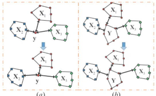
Figure 1. PSD (left) and SSD (right) Metric learning Inspired by the success of metric learning in PPD based classification, the performance of PSD and SSD based clas-sification can also be boosted by metric learning. As shown in the upper part of Fig. 1(a), the query image y (repre-sented as a red dot) has the same class label as template set
X1 (represented as a red hull) but it will be misclassified
since it has a closer PSD to setX2. If a proper metric
learn-ing method can be developed, it is possible that with the new distance metric, the PSD betweenyandX1is smaller than
that betweenyandX2, and consequentlyycan be correctly
classified, as shown in the bottom part of Fig. 1(a). Similar anticipation goes to the metric learning of SSD based clas-sification, as illustrated in Fig. 1(b), where the query set
Y can be correctly classified with some proper SSD based distance metric.
With the above considerations, in this paper we propose two novel metric learning models, PSD metric learning (PS-DML) and SSD metric learning (SS(PS-DML), to enhance the performance of PSD and SSD based classification. One im-age (or imim-age set) and one similarly labeled imim-age set con-struct a positive pair, while one image (or image set) and one differently labeled set construct a negative pair. Then the PSDML and SSDML problems are formulated as a sam-ple pair classification problem. Each samsam-ple pair is charac-terized by the covariance matrix of its two samples, and a covariance kernel is introduced. A discriminative function is then proposed for sample pair classification, and finally the PSDML and SSDML can be solved by using an SVM model. The proposed PSDML and SSDML methods can ef-fectively improve the performance of PSD and SSD based classification, and are much more efficient than state-of-the-art metric learning methods.
The main abbreviations used in this paper are summa-rized in the following Table 1.
Table 1. The main abbreviations used in this paper PPD point to point distance PSD point to set distance SSD set to set distance
PSDML point to set distance metric learning SSDML set to set distance metric learning
2. Set based distances
Before distance metric learning, we need to first define how the distance is measured. In this section, we describe how an image set is modeled, and how the corresponding point-to-set and set-to-set distances are defined.
2.1. Image set model
An image set is usually represented by a hull, i.e., a sub-space spanned by all the available samples in the set. The hull of a set of samplesD = [d1...,di...,dn]is defined as
H(D) = {Da}, wherea = [a1;...;ai, ...;an]. Usually, Pa
i = 1is required andaiis required to be bounded:
H(D) ={P
diai|Pai= 1,−τ1≤ai≤τ2} (1)
Ifτ1 = −inf andτ2 = inf,H(D)is an affine hull [26].
τ1= 0andτ2 = 1,H(D)is a convex hull [26]. Ifτ1 = 0
andτ2<1,H(D)is a reduced convex hull [5].
To rule out the meaningless points which are too far from the sample mean, the regularized affine hull (RAH) [35] is defined as follows to model an image set:
H(D) =nP
diai|Pai= 1,kaklp≤σ o
(2)
2.2. Point-to-set distance (PSD)
Given a sample x and a set of samples D, a point to set distanced(x,D)betweenxandD can be defined as follows:
d(x,D) =kx−Dˆak2 (3)
where ˆa = arg minakx−H(D)k
2
2. When H(D) is a
hull, the solution ofminakx−H(D)k22can be easily ob-tained by least square regression as DTD−1DTx
if DTD is non-singular, or by ridge regression
DTD+λI−1
DTxifDTDis (nearly) singular. To make the PSD more accurate for classification, a pro-jection matrixP can be introduced to project the samples into a desired space. The corresponding PSD distance, de-noted bydM(x,D), is then defined as:
dM(x,D) =kP(x−Dˆa)k 2 2 = (x−Daˆ)TPTP(x−Daˆ) = (x−Daˆ)TM(x−Daˆ) (4)
whereaˆ= arg minakP(x−Da)k
2 2, and
M =PTP, (5)
Whenaˆ is obtained, we can form a sample pair(x,Daˆ). Clearly, the PSD dM(x,D) defined in Eq. (4) can be viewed as a Mahalanobis distance [10] betweenxandDaˆ, and the matrixM is always semi-positive definite.
In PSD based classification, the distance between the query sample y and the template set of each class
X1,X2, ...,Xc (c is the number of classes) needs to be computed first. Suppose that the nearest subspace classifier (NSC) is used. GivenM, for classi, we haveˆai =Wiy, where
Wi= XiTM Xi+λI −1
XiTM. (6) and then the PSD betweenyand setXiis:
dM(y,Xi) = (y−Xiˆai)TM(y−Xiˆai). (7) The class with the minimal PSD is assigned to y:
Label(y) = arg mini{dM(y,Xi)}.
Compared with the nearest convex hull/affine hull clas-sifier (NCH/NAH), which needs to solve c quadratic pro-gramming problems for the query sample y, NSC only needs to compute a set of linear projections of y with
Wi, i= 1,2, ..., c. Hence, NSC is much more efficient than NCH and NAH.
2.3. Set-to-set distance (SSD)
Given two image setsD1andD2, the set-to-set distance
(SSD) between them can be defined as follows:
d(D1,D2) = D1aˆ−D2 ˆb 2 2 (8)
whereˆaandˆbcan be solved by:
(a,ˆ ˆb) = arg mina,bkH(D1)−H(D2)k 2
2 (9)
When convex/affine/regularized constraints are imposed on the coefficient vectors a and b, respectively, the corre-sponding distances are convex hull based image set dis-tance (CHISD) [5], affine hull based image set disdis-tance (AHISD) [5] and regularized nearest points (RNP) [35], re-spectively. In [35], it has been shown thatl2-norm
regular-ized affine hull is much faster and can achieve comparable performance to convex/affine/sparse constraints. Given a linear projection matrixP, the RNP model is:
mina,bkP(D1a−D2b)k 2 2+λ1kak 2 2+λ2kbk 2 2 s.t.P ai= 1,Pbi= 1 (10) By solving Eq. (10), the SSD in Eq. (8) becomes:
dM(D1,D2) = P(D1aˆ−D2 ˆb) 2 2 = (D1ˆa−D2ˆb)TM(D1ˆa−D2ˆb) (11)
In SSD based classification, given a query image setY, the SSD between it and each template setXi, i= 1,2, ..., c, is computed as
dM(Y,Xi) = (Yˆa−Xiˆbi)TM(Yaˆ−Xiˆbi). (12)
Y can then be classified byLabel(Y) =l(Xˆi), whereˆi=
arg mini{dM(Y,Xi)}.
3. Distance metric learning
With the definitions in Section 2, we can then design the metric learning algorithms for PSD and SSD based classifi-cation.
3.1. Point-to-set distance metric learning (PSDML)
According to Eq. (7), the matrix M plays a critical role in the final distance dM(y,Xi). It is expected that a good M can be learned from the training sample sets{X1,X2, ...,Xc}, so that the PSD between a query sample
yand the setXl(y)can be reduced, while the PSD between
yand the other setsXj, j6=l(y), can be enlarged, where
l(y)is the label ofy.
To achieve this goal, with the given training data sets
model: minM,a l(xi),aj,ξijN,ξPi,bkMk 2 F+ν( P i,jξ N ij+ P iξ P i ) s.t. dM(xi,Xj) +b≥1−ξijN, j6=l(xi); dM(xi,Xl(xi)) +b≤ −1 +ξ P i ; M<0,∀i, j, ξN ij≥0, ξiP ≥0 (13)
wherek·kF denotes the Frobenius norm,al(xi)andajare coefficients vector for Xl(xi)andXj,b is the bias andν is a positive constant. ξiP andξijN are slack variables for positive and negative pairs. dM(xi,Xl(xi)) is the PSD distance from xi to the set it belongs to (i.e., the PSD of positive pairs), where l(xi) is the class label of xi, and
dM(xi,Xj), j6=l(xi), is the PSD fromxito other classes (i.e., the PSD of negative pairs).
Eq. (13) is a joint optimization problem of M and
{al(xi),aj}. Like the strategy adopted in many multi-variable optimization problems, we minimize Eq. (13) by optimizingM and{al(xi),aj}alternatively. WhenM is fixed, {al(xi),aj}are solved for all the training samples. Note that here the“leave-one-out” strategy is used to com-puteal(xi). That is, X¯l(xi) is the training sample set of classl(xi)but excluding samplexi. Then the positive pairs are formed as(xi,X¯l(xi)aˆl(xi))and the negative pairs are formed as(xi,Xj,j6=l(xi)aˆj,j6=l(xi)). We label the negative pair as “+1” and the positive pair is set as “-1”.
Let us denote by zi = (zi1,zi2) a generated sample
pair. The covariance matrix of the two samples in zi is
Ci = (zi1−zi2)(zi1−zi2)T. Suppose that we generated
nstraining sample pairs, and thus we havenscovariance matricesCi, i= 1,2, ..., ns. We labelCi as “+1” or “-1” based on the label of zi, and define the following kernel function to measure the similarity betweenCiandCj:
k(Ci,Cj) =tr(CiCj) =<Ci,Cj > (14) wheretr(·)is the trace operator of a matrix and< ·,· >
means the inner product of matrices.
Suppose that we have a query sample pair, denoted by
z = (z1,z2). The covariance matrix ofzis denoted byC.
We introduce the following discriminative function to judge whetherzis positive or negative:
f(C) =P iβilik(Ci,C) +b =P iβili<Ci,C >+b =<P iβiliCi,C>+b (15)
whereliis the label of pairzi, andβiis a weight. Let
M =P
iβiliCi. (16) Then we havef(C) =<M,C>+b.
The metric learning problem in Eq. (13) can then be converted into the following problem:
minM,b,ξkMk 2 F +ν P iξi s.t. li(<M,Ci >+b)≥1−ξi, ξi≥0 (17)
The Lagrange dual problem of the metric learning problem in Eq. (17) is:
maxβ−12Pi,jβiβjliljk(Ci,Cj) +νPiβi
s.t.0≤βi≤µ,Piβili = 0
(18) Obviously, the minimization in Eq. (18) can be easily solved by the support vector machine (SVM) solvers such as LIBSVM [7]. Onceβ = [β1, ..., βi, ..., βns]is obtained by solving Eq. (18),Mcan be obtained by Eq. (16). With
M, the distance between two samples z1 andz2 can be
computed as:
dM(z1,z2) = (z1−z2)TM(z1−z2)
=tr(M C) =<M,C> (19)
If we further requiredM(z1,z2)to be a Mahalanobis
dis-tance metric,M should be semi-positive definite. Similar to Xing et al.’s MMC [33] and Globerson et al.’s MCML [12], we can compute the singular value decomposition (SVD) ofM = UΛV , whereΛis the diagonal matrix of eigenvalues, and then set the negative eigenvalues inΛ to 0, resulting in a new diagonal matrixΛ+. Finally, we let
M+=UΛ+V be the learned matrix.
OnceMis computed,{al(xi),aj}are then updated, and theM is further updated, and so on. The proposed point-to-set distance metric learning (PSDML) algorithm is sum-marized in Table 2. The PSDML can be coupled with PSD based classifiers such as NSC [8], NCH [26] and NAH [26] for classification. In this paper, we use NSC since it is much more efficient than NCH and NAH.
Table 2. Algorithm of point to set distance metric learning (PS-DML)
Input:X = [X1,X2, ...,Xc], labell,λandν Output:M
1 InitializeM =I
2 While iteration number< num
3 ComputeWi,i= 1, ..., cby Eq. (6); 4 Construct positive and negative sample pairs; 5 Solve Eq. (18) by SVM solver;
6 UpdateMby Eq. (16); 7 End
3.2. Set-to-set distance metric learning (SSDML)
With the SSD defined in Eq. (8), we can also learn a ma-trixM from the training sample sets{X1, ...,Xi, ...,Xn} so that the SSD between sets with the same label can be re-duced, while the SSD between sets with different labels can be enlarged. The proposed set-to-set distance metric learn-ing (SSDML) model is formulated as follows:minM,a i,aj,ak,ξPik,ξPik,bkMk 2 F+ν( P i,kξ P ik+ P i,jξ N ij) s.t. dM(Xi,Xj) +b≥1−ξijN, l(Xi)6=l(Xj); dM(Xi,Xk) +b≤ −1 +ξikP, l(Xi) =l(Xk); M<0,∀i, j, k, ξijN≥0, ξikP ≥0 (20)
whereai,aj,ak are the coefficients vector for image sets
Xi,Xj,Xk;l(Xi)means the label of setXi, andξPik,ξ N ij are the slack variables for positive pairs and negative pairs. The principles and main procedures of SSDML are sim-ilar to the PSDML in Section 3.1. We solve Eq. (20) by optimizing M and {ai,aj,ak} alternatively. When M is fixed,{ai,aj,ak}are updated to construct positive and negative sample pairs. When the sample pairs are given, the updating of matrixM can also be converted into the problem in Eq. (17). The algorithm of SSDML is sum-marized in Table 3. Note that the work in [32] relies on CHISD [5] and SANP [16]. As RNP [35] is much faster than convex/sparse hull based SSD computation, we choose it to learn the Mahalanobis distance metric based on l2
-norm regularized affine hull.
Table 3. Algorithm of set to set distance metric learning (SSDML) Input: Training image setsX= [X1,X2, ...,Xn],
labell,λ1,λ2andν
Output:M
1 InitializeM =I
2 While iteration number< num
3 Compute SSD for each image setXiby Eq. (10); 4 Construct positive and negative sample pairs; 5 Solve Eq. (18) by SVM solver;
6 UpdateM by Eq. (16); 7 End
3.3. Discussions
There are close relationships between the proposed PS-DML/SSDML and SVM. The geometric interpretation of
ν-SVM is to find the closest points in two (reduced) convex hulls [4]. Given two classes X1 andX2, the SVM is to
solve the following problem [4]:
minkX1a1−X2a2k 2 2 s.t.Pa 1i= 1,Pa2j = 1,0≤a1i, a2j≤µ (21) It can be easily found that the associated discrimination function of SVM isf(y) =wTy+b, wherew= (X
1a1−
X2a2)/2, p = (X1a1+X2a2)/2, b = −wTp =
(a2TX2TX2a2−a1TX1TX1a1)/4.
Then we have the following observation:
f(y) =wTy+b =(X1a1−2X2a2)Ty+a2TX2TX2a2−a1TX1TX1a1 4 =ky−X2a2k 2 2−ky−X1a1k 2 2 4 =d(y,X2)−d(y,X1) 4 (22)
Hence, similar to PSD based classification, the discrimi-native function of SVM actually uses the distance between the test sampleyand each class. Iff(y) ≥0, theny be-longs to the first class. If f(y) < 0, theny belongs to
the second class. The difference, however, lies in that PSD based classifiers (e.g., NSC, NCH and NAH) solvea1and
a2for each test sample while SVM learnsa1anda2from
the training set by classification loss minimization and mar-gin maximization. The conventional PSD based classifiers ignore the training label information in computinga1and
a2. With metric learning, PSDML can further utilize the
class label to learn a discriminative metric for the point-to-set distance, and thus may result in better classification performance.
For set based classification, SVM can not be directly used. Actually, given two sets, SVM considers each set as one class and the distance between two classes is used as the SSD, which corresponds to CHISD [5]. Hence, it still ignores the discriminative information in calculating SSD, and is essentially different from the proposed SSD metric learning method.
Additionally, we formulate both PSDML and SSDML as a sample pair classification problem, which can be solved by standard SVM solvers. This makes metric learning very efficient.
4. Experimental result and analysis
We verify the performance of PSDML and SSDML on various visual classification tasks. In Section 4.1, we test PSDML on gender classification, digit recognition, object categorization and face recognition, while in Section 4.2, we test SSDML on video-to-video based face recognition.
4.1. PSDML experiments
4.1.1 Parameter setting and competing methods There are two parameters in PSDML, i.e.,λin Eq. (6) and
ν in Eq. (17). For SSDML, there are three parameters, i.e.,
λ1andλ2in Eq. (10) andν in Eq. (17). For both PSDML
and SSDML,ν in Eq. (17) is set to the default value 1 in LIBSVM. For PSDML,λis chosen by cross-validation on the training set. For SSDML,λ1andλ2are fixed as 0.001
and 0.1, respectively.
We compare PSDML with four state-of-the-art metric learning methods (LMNN [31], ITML [10], NCA [13] and MCML [12]), three PSD based classifiers (NSC [8], NCH [26] and NAH [26]), the classical nearest neighbor classi-fier (NNC) and SVM. The Matlab source codes of LMNN, ITML, NCA, and MCML are obtained from the original au-thors, and we used the SVM toolbox from [7]. We imple-mented NNC, NCH, NAH and NSC. The parameters of the competing methods are tuned for their best results.
4.1.2 Gender classification
A non-occluded subset (14 images per subject) of the AR dataset [22] is used, which consists of 50 male and 50 fe-male subjects. We use the images from the first 25 fe-males
and 25 females for training, and the remaining images for testing. The images were cropped to 60×43. PCA was used to reduce the dimension of each image to 30 and 50, respec-tively. The experimental results listed in Table 4 show that PSDML gets the highest accuracy and improves the perfor-mance of PSD based classifiers (NSC, NCH and NAH).
Table 4. Accuracy (%) on gender classification
dim. NN NSC NCH NAH SVM
30 90.6 92.1 91.1 91.7 92.1 50 90.3 93.3 91.4 84.3 91.0 dim. LMNN ITML NCA MCML PSDML
30 91.3 90.8 91.4 90.7 93.7 50 91.0 90.7 91.4 92.1 95.4
4.1.3 Digit recognition
Three handwritten digit datasets, Semeion [2], USPS [17] and MNIST [21], are used here.
Semeion: The Semeion dataset [2] has 1,593 handwrit-ten digits from around 80 persons. Each sample is a 16×16 binarized image. The recognition rate on the raw features is shown in Table 5. On this dataset, the performance of NSC is much better than NNC. PSDML gets a recognition accu-racy of 95.9%, which is the highest among all the methods used in comparison.
Table 5. Accuracy (%) on Semeion
dim. NN NSC NCH NAH SVM
256 91.4 94.2 94.1 92.5 93.4 dim. LMNN ITML NCA MCML PSDML
256 93.9 93.5 93.9 90.0 95.9
USPS: The USPS dataset includes 7,291 training and 2,007 testing images [17]. Each sample is a 16×16 im-age. The experimental results on three dimensions (100, 150, 256) are shown in Table 6. We see that the results of NNC and NSC are similar. PSDML achieves the high-est accuracy on different dimensions and its performance is comparable to other state-of-the-art metric learning meth-ods.
Table 6. Accuracy (%) on the USPS
dim. NN NSC NCH NAH SVM
100 94.9 94.3 88.2 91.8 92.3 150 94.8 94.5 89.3 91.9 92.7 256 94.6 94.3 89.7 91.8 92.7 dim. LMNN ITML NCA MCML PSDML
100 95.2 95.0 95.1 95.2 95.4 150 95.2 95.1 95.0 95.1 95.3 256 95.0 94.9 94.8 94.9 95.2
MNIST: The MNIST [21] dataset contains a training set of 60,000 samples and a test set of 10,000 samples. There
are 10 classes of images, and the size of each image is 28×28. We randomly select 200 samples per class for train-ing and the image dimension is reduced to 100 by PCA. Ten random experiments are conducted and the average recog-nition rate is shown in Table 7. Again, PSDML performs the best among all methods.
Table 7. Accuracy (%) on MNIST
dim. NN NSC NCH NAH SVM
100 93.3 95.2 96.0 94.0 95.7 dim. LMNN ITML NCA MCML PSDML
100 95.0 93.4 93.5 90.1 96.3 4.1.4 Object categorization
The 17 category OXFORD flower dataset [23] is used. It contains 17 species of flowers with 80 images for each class. Theχ2distance matrices of seven features (i.e., HSV, HOG,
SIFTint, SIFTbdy, color, shape and texture vocabularies) are directly used as the input and the experiments are con-ducted based on the three predefined training, validation, and test splits. We test the performance of PSDML on each feature and the results are shown in Table 8. From the re-sults we see that PSDML achieves the highest accuracy on all the seven features.
Table 8. Accuracy (%) on the 17 category OXFORD flowerers
Features NN NSC NAH NAH SVM
Color 52.3±2.2 55.4±2.7 55.2±2.8 56.3±2.8 56.9±2.6 Shape 53.7±3.5 66.5±2.1 66.7±2.0 63.4±1.3 60.0±2.9 Texture 31.9±3.6 52.4±2.1 52.4±1.5 45.5±1.8 47.8±3.4 HSV 52.0±2.6 59.2±2.3 59.4±2.3 57.2±3.5 57.0±2.9 HOG 36.9±1.7 51.6±2.5 51.8±2.9 47.6±2.6 47.3±1.9 SIFTint 58.7±2.1 66.5±1.3 66.5±1.4 64.5±1.0 59.7±1.0 SIFTbdy 51.7±0.9 57.6±2.3 57.7±2.2 57.6±2.8 47.5±2.8
Features LMNN ITML NCA MCML ISDML
Color 53.1±2.5 53.5±2.6 52.8±2.8 54.1±2.758.8±4.0 Shape 50.1±1.0 55.0±1.4 54.5±2.0 55.5±1.567.8±2.0 Texture 35.5±3.0 36.2±2.5 33.8±2.6 34.5±2.055.0±1.3 HSV 54.8±2.7 53.5±3.0 54.0±2.9 52.9±3.161.6±3.2 HOG 38.3±1.1 37.5±2.5 38.2±2.5 38.7±2.855.0±5.9 SIFTint 60.0±3.4 61.2±1.9 59.8±1.5 60.4±1.369.1±1.8 SIFTbdy 53.3±4.1 54.2±2.5 53.3±2.9 53.3±2.160.6±4.0 4.1.5 Face recognition
We then test the performance of PSDML on face recog-nition. As in [31], the Extended Yale B database [11] is used here. In addition, the FERET database [25] is also used since the images have huge pose variations, making it a good test-bed for metric learning methods.
Extended YaleB: The Extended YaleB database contains 2,414 frontal face images of 38 persons [11]. There are about 64 images for each subject. The original images were
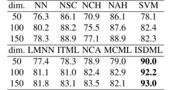
cropped to 192×168 pixels. This database has varying il-luminations and expressions. A randomly generated matrix from a zero-mean normal distribution is is used to project the face image onto a 504-dimensional vector. We randomly choose 15 samples per subject for training and the rest im-ages are used for test. PCA is used to reduce the dimension to 50, 100 and 150, respectively. On this database, the per-formance of NSC is much better than NNC. Compared with NSC, PSDML improves the recognition rate by about 4%
and it works much better than other competing methods. Table 9. Accuracy (%) on the Extended YaleB database
dim. NN NSC NCH NAH SVM
50 76.3 86.1 70.9 86.1 78.1 100 80.2 88.2 75.5 87.6 82.4 150 78.3 88.9 77.1 88.9 82.3 dim. LMNN ITML NCA MCML ISDML
50 77.4 78.3 78.9 79.0 90.0 100 81.1 81.0 82.4 82.9 92.2 150 81.8 83.1 83.5 82.1 93.0
FERET: The FERET face database is a large and popu-lar database for evaluating state-of-the-art face recognition algorithms [25]. We use a subset of the database that in-cludes 1,400 images from 200 individuals (each has 7 im-ages). It consists of the images whose names are marked with two character strings:“ba”, “bj”, “bk”, “bd”,“be”,“bf”, “bg”. This subset involves variations in facial expression, illumination, and pose. The facial portion of each image was automatically cropped based on the location of eyes and mouth, and the cropped image was resized to60×50
pixels and further pre-processed by histogram equalization. We randomly select four images per subject as the train-ing set and the remaintrain-ing images are used as the test set. The recognition rates are shown in Table 10. In this dataset, the performance of NSC is worse than NNC. This is be-cause there are great pose variations in this subset, and thus using hull to model the image set is not suitable. By metric learning, however, the classification rate can be improved greatly. The result of PSDML is much better than LMNN, ITML, NCA and MCML, which validates the effectiveness of our algorithm.
4.1.6 Time comparison
To show the efficiency of PSDML, we compare the training time of different metric learning methods. All algorithms are run in an Intel(R) Core(TM) i7- 2600K (3.4GHz) PC. The average training time on the MNIST dataset is listed in Table 11. We see that PSDML is much faster than other metric learning methods. In particular, it is nearly500times faster than MCML.
Table 10. Accuracy (%) on the FERET
dim. NN NSC NCH NAH SVM
50 40.5 38.9 37.6 38.9 45.8 100 48.0 42.4 41.5 42.4 59.5 150 48.8 43.7 42.6 43.7 64.6 dim. LMNN ITML NCA MCML PSDML
50 60.0 61.5 59.5 60.5 64.0 100 62.7 63.8 61.6 63.3 67.8 150 63.5 64.8 62.0 64.5 67.8
Table 11. Training time (s) on the MNIST Methods LMNN ITML NCA MCML PSDML run time 75.9 141.0 3885.1 11825.1 24.7
4.2. SSDML experiments
We then test SSDML for set-to-set based classifica-tion tasks. The benchmark YouTube Celebrities dataset is used. In this experiment, we compare SSDML with those SSD based classification methods (CHISD [5], AHISD [5], SANP [16], RNP [35], MMD [29] and MDA [28]) and set-to-set similarity based methods (MSM [34] and DCC [20]). The source codes of these methods are from the original authors and we tune the parameters for their best results.
The Youtube Celebrities [20] is a large scale video dataset for face tracking and recognition, consisting of 1,910 video sequences of 47 celebrities collected from YouTube. As the videos were captured in unconstrained en-vironments, the recognition task becomes much more chal-lenging due to large variations in pose, illumination and ex-pressions. The face in each frame is detected by the Viola-Jones face detector and resized to a 30×30 grayscale image. The intensity value is used as feature. Three video se-quences per subject are selected for training and six for test-ing. Five-fold cross validation is used. The experiments for 50, 100, 200 frames per set are conducted. The result is shown in Table 12. We can see that SSDML outperforms all the other methods on different frames per set.
Table 12. Recognition rates on YouTube (%)
Methods 50 100 200 MSM [34] 54.8±8.7 57.4±7.7 56.7±6.9 DCC [20] 57.6±8.0 62.7±6.8 65.7±7.0 MMD [29] 57.8±6.6 62.8±6.2 64.7±6.3 MDA [28] 58.5±6.2 63.3±6.1 65.4±6.6 AHISD [5] 57.5±7.9 59.7±7.2 57.0±5.5 CHISD [5] 58.0±8.2 62.8±8.1 64.8±7.1 SANP [16] 57.8±7.2 63.1±8.0 65.6±7.9 RNP [35] 59.9±7.3 63.3±8.1 64.4±7.8 SSDML 61.9±7.3 65.0±8.1 67.0±7.1
5. Conclusion
We extended the point-to-point distance metric learning to point-to-set distance metric learning (PSDML) and set-to-set distance metric learning (SSDML). Positive and neg-ative sample pairs were generated from training sample sets by computing point-to-set distance (PSD) and set-to-set dis-tance (SSD). Each sample pair was represented by its co-variance matrix and a coco-variance kernel based discrimina-tion funcdiscrimina-tion was proposed for sample pair classificadiscrimina-tion. Finally, we showed that the proposed metric learning prob-lem can be efficiently solved by SVM solvers. Experiments on various visual classification problems demonstrated that the proposed PSDML and SSDML methods can effectively improve the performance of PSD and SSD based classifi-cation. Compared with the state-of-the-art metric learning methods such as LMNN, ITML and MCML, the proposed method can achieve better classification accuracy and is sig-nificantly faster in training.
Acknowledgments
This work is partly supported by the HK RGC GRF grant (PolyU 5313/12E) and by NSFC under Grant 61271093.
References
[1] V. Ablavsky and S. Sclaroff. Learning parameterized his-togram kernels on the simplex manifold for image and action classification. InICCV 2011.
[2] A. Asuncion and D. J. Newman. Uci machine learning repos-itory, 2007.
[3] M. Bilenko, S. Basu, and R. J. Mooney. Integrating con-straints and metric learning in semi-supervised clustering. In
ICML 2004.
[4] D. Burges. A geometric interpretation ofν-svm classifiers.
NIPS 2000.
[5] H. Cevikalp and B. Triggs. Face recognition based on image sets. InCVPR 2010.
[6] H. Cevikalp, B. Triggs, and R. Polikar. Nearest hyperdisk methods for high-dimensional classification. InICML 2008. [7] C.-C. Chang and C.-J. Lin. Libsvm: a library for support vector machines. ACM Transactions on Intelligent Systems and Technology (TIST), 2(3):27, 2011.
[8] J.-T. Chien and C.-C. Wu. Discriminant waveletfaces and nearest feature classifiers for face recognition. TPAMI, 24(12):1644–1649, 2002.
[9] R. G. Cinbis, J. Verbeek, and C. Schmid. Unsupervised met-ric learning for face identification in tv video. InICCV 2011. [10] J. V. Davis, B. Kulis, P. Jain, S. Sra, and I. S. Dhillon.
Information-theoretic metric learning. InICML 2007.
[11] A. S. Georghiades, P. N. Belhumeur, and D. J. Kriegman. From few to many: Illumination cone models for face recog-nition under variable lighting and pose. TPAMI, 23(6):643– 660, 2001.
[12] A. Globerson and S. Roweis. Metric learning by collapsing classes. InNIPS 2006.
[13] J. Goldberger, S. Roweis, G. Hinton, and R. Salakhutdinov. Neighbourhood components analysis. InNIPS 2004. [14] M. Guillaumin, J. Verbeek, and C. Schmid. Is that you?
met-ric learning approaches for face identification. InICCV 2009. [15] M. Guillaumin, J. Verbeek, and C. Schmid. Multiple instance metric learning from automatically labeled bags of faces. In
ECCV 2010.
[16] Y. Hu, A. S. Mian, and R. Owens. Sparse approximated nearest points for image set classification. InCVPR 2011. [17] J. J. Hull. A database for handwritten text recognition
re-search.TPAMI, 16(5):550–554, 1994.
[18] N. Jiang, W. Liu, and Y. Wu. Order determination and sparsity-regularized metric learning adaptive visual tracking. InCVPR 2012.
[19] D. Kedem, S. Tyree, K. Weinberger, F. Sha, and G. Lanckriet. Non-linear metric learning. InNIPS 2012.
[20] T. Kim, J. Kittler, and R. Cipolla. Discriminative learning and recognition of image set classes using canonical correla-tions.TPAMI, 29(6):1005–1018, 2007.
[21] Y. LeCun and C. Cortes. The mnist database of handwrittn digits.http://yann.lecun.com/exdb/mnist/. [22] A. Martinez. The ar face database. CVC Technical Report,
24, 1998.
[23] M.-E. Nilsback and A. Zisserman. A visual vocabulary for flower classification. InCVPR 2006.
[24] S. Parameswaran and K. Weinberger. Large margin multi-task metric learning. InNIPS 2010.
[25] P. J. Phillips, H. Moon, S. A. Rizvi, and P. J. Rauss. The feret evaluation methodology for face-recognition algo-rithms.TPAMI, 22(10):1090–1104, 2000.
[26] P. Vincent and Y. Bengio. K-local hyperplane and convex distance nearest neighbor algorithms.NIPS 2002.
[27] F. Wang, W. Zuo, L. Zhang, D. Meng, and D. Zhang. A kernel classification framework for metric learning.
arXiv:1309.5823, 2013.
[28] R. Wang and X. Chen. Manifold discriminant analysis. In
CVPR 2009.
[29] R. Wang, S. Shan, X. Chen, and W. Gao. Manifold-manifold distance with application to face recognition based on image set. InCVPR 2008.
[30] Z. Wang, Y. Hu, and L.-T. Chia. Image-to-class distance metric learning for image classification. InECCV 2010. [31] K. Q. Weinberger, J. Blitzer, and L. K. Saul. Distance metric
learning for large margin nearest neighbor classification. In
NIPS 2006.
[32] Y. Wu, M. Minoh, M. Mukunoki, and S. Lao. Set based discriminative ranking for recognition. InECCV 2012. [33] E. P. Xing, A. Y. Ng, M. I. Jordan, and S. Russell.
Dis-tance metric learning, with application to clustering with side-information. InNIPS 2002.
[34] O. Yamaguchi, K. Fukui, and K. Maeda. Face recognition using temporal image sequence. InFG 1998.
[35] M. Yang, P. Zhu, L. Van Gool, and L. Zhang. Face recogni-tion based on regularized nearest points between image sets. InFG 2013.
[36] G.-T. Zhou, T. Lan, W. Yang, and G. Mori. Learning class-to-image distance with object matchings.