Best fit model selection for spatial differences (regression) in the profitability
analysis of precision phosphate (P) application to winter cereals in Precision
Agriculture (PA)
By
Hough, EC; Nell, WT; Maine, N; Groenewald, JA & van der Rijst, M
Contributed Paper presented at the Joint 3rd African Association of Agricultural Economists (AAAE) and 48th Agricultural Economists Association of South Africa
Best fit model selection for spatial differences (regression) in
the profitability analysis of precision phosphate (P) application
to winter cereals in Precision Agriculture (PA).
EC Hough
1, WT Nell
2, N Maine
3, JA Groenewald
4& M van der Rijst
51
Agricultural Economist, MKB, PO Box 30, Moorreesburg, 7310. [email protected] 2
Lecturer Department of Agricultural Economics, University of the Free State, P.O. Box 339, Bloemfontein 9300. [email protected]
3
Director, Agricultural Development Programmes, City of Tshwane, P.O. Box 440, Pretoria, 0001. [email protected]
4
Professor Extraordinary, Department of Agricultural Economics, University of the Free State, P.O. Box 339, Bloemfontein 9300. [email protected]
5
Biometrician, Agricultural Research Council, Biometry Unit, Private Bag X5013, Stellenbosch, 7599. [email protected]
Best fit model selection for spatial differences (regression) in
the profitability analysis of precision phosphate (P) application
to winter cereals in Precision Agriculture (PA).
Abstract
Phosphates (P) are an important nutrient required by every living plant and animal cell, and deficiencies in soils could cause limited crop production, thereby reducing profitability. Phosphates are also a primary nutrient essential for root development and crop production, and are needed in the tissues of a plant where cells rapidly divide and enlarge. Precision agriculture (PA) could assist the farmer in applying the correct amount of P to the part of the field where it is required most. Variable rate technology (VRT) is a potential tool that can help with the development of strategies for phosphate fertilizer management.
On-field trials were conducted on a commercial farm in the Western Cape Province; As many as five soil types occur on each field studied, and three crops – wheat, canola and barley - are grown in rotation. One half of each field was planted using VRT (PA), while constant application (SR) was used on the other half. The objective was to determine whether spatial econometric models are more accurate than traditional ordinary least squares (OLS) models in predicting the profitability impact of P on PA.
There are significant differences to be observed between the results obtained with the OLS, Spatial Error (SER) and restricted maximum-likelihood (REML) models. All the measures of goodness of fit indicated an increase in fit from the OLS to the SER model, with the best fit being achieved with the REML model, implying that the use of this model resulted in more accurate estimates.
Key terms: Precision agriculture, variable-rate phosphate application, single rate phosphate application, profitability, spatial differences, restricted maximum-likelihood model (RELM), spatial regression, best fit model selection, South Africa.
1. Introduction
Swinton and Lowenberg-DeBoer (1998) reported that agriculture is becoming an industry based on knowledge, and that the ability to learn efficiently is a key factor in ensuring profitability in this sector. According to Gandonou, Stombaugh, Dillon and Shearer (2001), agriculture is increasingly becoming a computerized, information-based industry. The best example of this trend is the evolution of precision agriculture (PA). PA is an emerging technology that prescribes inputs based on site-specific soil and crop characteristics (Snyder, Schroeder, Havlin & Kluitenberg, 1996).
New intelligent technologies lead by the utilisation of information technologies, are changing traditional production processes. These intelligent technologies, in combination with the determination of “position and time”, are much more complex than just dividing fields into management zones (Auernhammer, 2002). Khanna, Epouche and Hornbaker (1999) are of the opinion that the developments in computer, satellite and agricultural equipment technology enable farmers to undertake site-specific crop management instead of relying on whole-field management. This development enables farmers also to make more precise decisions about the application of inputs in order to avoid deficiencies and excesses in input-use. Snyder et al. (1996) stated that factors influencing crop yield can now be spatially measured, monitored and managed in order to ensure that inputs are only applied where they are most needed.
Phosphorus (P) promotes growth in plants and animals and thus the importance of P cannot be over-emphasized in agriculture. Deficient P can cause low yield and poor quality of crops and pastures. Phosphate rock provides the phosphorous elements of nitrogen, phosphate and potassium (N:P:K) in the most efficient mix to ensure good growth in plants (Florida Institute of Phosphate Research, 2004).
According to a study undertaken by Robinson (2005) near Cleveland, Mississippi, it was found that in some areas in farm fields the plants were stunted and these areas also did not yield well. By adding a yield monitor to a combine, the problem areas were identified. Soil samples indicated very low levels of P and the decision was taken to try a
pre-plant application of Triple Super P. Satisfying the soil’s P needs by applying chicken manure can cost the producer $12,00 per pound of P applied. By applying the variable rate of P, the yield showed increases. This fact emphasizes the importance of addressing the specific sites where the problems are experienced.
Roberts, English and Larson (2002) reported that more precise placement of inputs with PA may increase farm profits. However, it is important to note that the key to farmer adoption is the profitability of the technology. It is predicted that more farmers will adopt PA techniques as soon as more scientific research results on the profitability of PA become available (Nell, Maine & Basson, 2006).
2. Literature
One of the key constraints identified on the widespread adoption of PA technology is the gap between data analysis and site-specific recommendations (Lambert, Lowenberg-DeBoer & Bongiovanni, 2003). Anselin, Bongiovanni and Lowenberg-Lowenberg-DeBoer (2004) also confirmed that the difficulties experienced in the analysis of spatial crop data are some of the key constraints. Spatially dense agronomic data such as the data obtained from yield monitors are often auto-correlated. This dependence among neighbouring observations violates the assumptions of classical statistical analysis (Lambert et al., 2003). Anselin etal. (2004) also stated that any observation obtained from yield monitors can clearly be correlated with the neighboring observations. Spatial regression analysis is one way of exploiting more fully the information contained in spatially dense data (Lambert et al., 2003). Spatial statistics assume that data are spatially correlated, for instance data obtained from yield monitors and site-specific data. If correlation is not accounted for in the analysis of these kinds of data, the results will be biased and misleading (Griffin, Brown & Lowenberg-DeBoer, 2005). Spatial analysis can include analysis with GIS and printing yield maps. It may be defined as “explicitly modeling the spatial auto-correlation in a spatial process model capable of making statistical inference” (Griffin & Lowenberg-DeBoer, 2008).
2.1Spatial auto-correlation
Spatial auto-correlation is described by Bongiovanni and Lowenberg-DeBoer (2001, cited in Maine, 2006) as a situation in which the dependent variable or error term at each location is correlated with observations on the dependent variable or values for the error term at other locations. It can be formally expressed as follows:
Cov [yi, yj] = ε [yiyj] = ε [Yi]. ε[Yj] = 0 For i ≠ j
Where i, j, refer to individual observations (locations) and yi (yj) is the value of the random variable of interest at that location.
When values such as yield data are obtained, spatial auto-correlation is caused by coincidence of similarities between location and these values. The reason for this is the fact that there is always a high chance that high or low values for a random variable will be surrounded by neighbouring observations with similar values.
2.2Spatial heterogeneity (Heteroscedasticity)
In the study by Maine (2006), spatial heterogeneity is described as a variation in the average relationships between X and Y over space. One can expect every point in space to have different relationships (LeSage, 1998). The results of this study reveal that the relationship between P as an X variable and yield (Y) varies from one point to the next or from one management zone to the next. When sample data are associated with a location, spatial dependence exists between the observations. The fact that underlying relationships may vary systematically over space, creates problems for regression and other econometric methods if these methods do not accommodate spatial variation in the relationships being modeled (LeSage, 1998). Lambert et al. (2003) stated that when general heterogeneity is ignored, VRT profit margins may appear less reliable.
3. Methodology
Data was collected by using the variable-rate (VR) application of phosphate (P), in comparison with the single-rate (SR) application The study was conducted in collaboration with Mr Gildenhuys (on-farm trials) in the Heidelberg district in the Western Cape, South Africa. Four fields, totaling 106 hectares (ha), were identified as research fields for the study. The main crops included in the study were wheat, canola and barley (3rd year). In each field as many as five soil types were found. Each field was divided into two halves. One half was planted by making use of VRT, and the other half was planted by conforming to the traditional farm management system or the standard rate (SR). The same crop was planted on both halves. Wheat, canola and barley were used in a crop rotation system. The results obtained are presented and compared using the traditional statistical analysis methods; the method of Ordinary Least Squares (OLS) and the spatial analysis method, the Spatial Error (SER) model (Table 1); the geo-statistical approach to spatial regression; and the Restricted Maximum Likelihood (REML) geo-statistics approach. The assumptions of classical statistical analyses are often violated when analysing spatial data (yield monitor data in this case) because of the correlation among neighbouring observations. By applying classical statistics to on-farm experiments, the assumption is made that observations are independent, but in the case of PA data this assumption of independence is untenable, as any yield monitor observation is clearly correlated to its neighbouring observations (Lambert, Lowenberg-DeBoer and Bongiovanni, 2003). Spatial auto-correlation is taken into account when spatial regression analysis is done and this method of analysis can overcome the limitations of classical statistical analysis.
This methodology was used to investigate the effect of the two treatments (VR and SR) on yield. The effect of the two treatments, VR and SR, are captured in a treatment (TRT) dummy variable, which assigns a value of 1 to VR and 0 to SR. Dummy variables to determine the effect for different soil types, as well as the treatment by soil type interactions are also included in a regression model. The aim is to determine whether yields vary spatially and this spatial variability is captured for different soil types.
The effect of spatial autocorrelation must be taken into account because of the nature of the data collected. The data are spatially correlated and it is essential to use the methodology that takes this into account. This is the reason why the spatial econometric analysis is so important in this study. PA is analysed as a package by using the Baseline Model (Treatment Model) and it is done by assessing the statistical significance of the estimated coefficients.
4. Objective
The objective with this paper is to determine whether spatial econometric models are more accurate than traditional ordinary least squares (OLS) models in predicting the profitability impact of PA on the yields and hence, profitability in the variable rate application of P.
5. Model specification
PA poses several challenges to both models and modelers as it does not just require simulation of the mean, but also a simulation of spatial variation. The model chosen should match the research objectives. For PA to succeed, one would expect the primary goal to be the ability of the model to simulate spatial variation. The accuracy of the model will determine how good the conclusions will be. In the case of the application of PA, regression has been used as primary test in most model tests. When using the regression approach, the model will produce useful results if the simulated output represents 70% to 80 % or more of the variation in the observed result (Sadler, Jones & Sudduth, 2007). One of the biggest challenges remain to link yields to soil conditions and to clearly establish the profitability of VRT fertiliser application. This complexity of yield response makes model specification difficult (Anselin etal., 2004).
5.1 Spatial and non-spatial models (OLS and ML)
Ordinary least squares (OLS) are a classical regression technique. When yield monitor data are analysed, it is important to take into account the spatial correlation of regression
residuals. When auto-correlation is ignored, the OLS estimates yielded will be inefficient and will bias the standard errors and t-test statistics (Anselin et al., 2004). Griffin et al. (2005) reported that OLS are unreliable in the presence of spatial variability, or in the cases of spatial auto-correlation and spatial heteroskedasticity. In spatial regression methods, maximum likelihood (ML) estimations are normally used.
5.2 Diagnostic tests for the Baseline Model
Maine (2006) reported that diagnostic tests on the OLS residuals determine the presence of spatial effects and also verify the optimal model. When the OLS model is run in conjunction with the weight matrix, the specification tests on spatial autocorrelation and heteroscedasticity (structural change) are acquired and this also suggests which model should be used (spatial error or spatial lag).
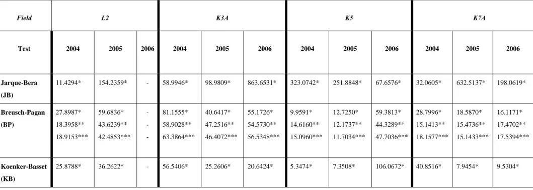
It was essential to determine if some of the assumptions of the classical linear regression models hold true before estimating the regression coefficient of data collected in this study. Some of these assumptions are that random variables are normally distributed and homoscedastic and that there is no autocorrelation and multicollinearity between variables. The Jarque-Bera (JB) test is used to determine normality in the error terms and thereby the hypothesis that the residuals are normally distributed is tested. The data collected for this study are cross-sectional in nature. Heterosceasticity is most common in these kinds of data. The Breusch-Pagan (BP) test is a diagnostic test done on a regression in order to determine the presence of heteroscedasticity in the error terms. The Koenker-Bassett (KB) test in the OLS model also confirms the presence of heteroscedasticity. In Table 1, a summary of these various diagnostic tests for normality, multicollinearity and heteroscedasticity are provided.
TABLE 1: DIAGNOSTIC TESTS FOR NORMALITY AND HETEROSCEDASTICITY
Field L2 K3A K5 K7A
Test 2004 2005 2006 2004 2005 2006 2004 2005 2006 2004 2005 2006 Jarque-Bera (JB) 11.4294* 154.2359* - 58.9946* 98.9809* 863.6531* 323.0742* 251.8848* 67.6576* 32.0605* 632.5137* 198.0619* Breusch-Pagan (BP) 27.8987* 18.3958** 18.9153*** 59.6836* 43.6239** 42.4853*** - - - 81.1555* 58.9028** 63.3864*** 40.6417* 47.2516** 46.4072*** 55.1726* 54.5730** 56.5348*** 9.9591* 14.6160** 15.0960*** 12.7250* 12.1737** 11.7034*** 59.3813* 44.3289** 47.7036*** 28.7996* 15.1413** 18.1577*** 18.5870* 15.4736** 15.1433*** 16.1171* 17.4702** 17.5394*** Koenker-Basset (KB) 25.8788* 36.2622* - 56.5406* 25.2606* 20.6424* 5.3474* 7.3508* 106.0672* 40.8516* 7.9454* 9.5304* *OLS model
**Spatial lag model ***Spatial error model
Table 1 shows that in the test for normality of errors in the Baseline Model using OLS, the highest JB value for 2004 was obtained for K5, namely 323.0742. For 2005 the highest value for K7A was 632.5137, and for 2006 it was 863.6531 for K3A. The JB values for each of the four fields for each of the three years are significant at a 1 % probability level. This indicates non-normality of the error terms. The larger the BP test, the greater the evidence against homoscedasticity. The highest BP value in the OLS model for 2004 is 81.1555 (K3A), for 2005 it was 59.6836 (L2), and for 2006 it was 59.3813 (K5), while the SER model produced values of 63.3864 (K3A) for 2004, 47.2516 (K3A) for 2005 and 56.5345 (K3A) for 2006. It is interesting to note that for the SER model, field K3A produced the highest BP values for the three years. The spatial error model was better for 2004 and 2006 due to the higher BP values, which provided even greater evidence against homoscedasticity. The highest KB value for 2004 was recorded for field K3A, namely 56.5406, for 2005 it was 36.2622 (L2), and for 2006 it was 106.0672 (K5). Dealing with heteroscedasticity in spatial data presents a problem, as no standard procedure has yet been developed in this regard. All the multicollinearity condition numbers are lower than 20, the recommended maximum condition number.
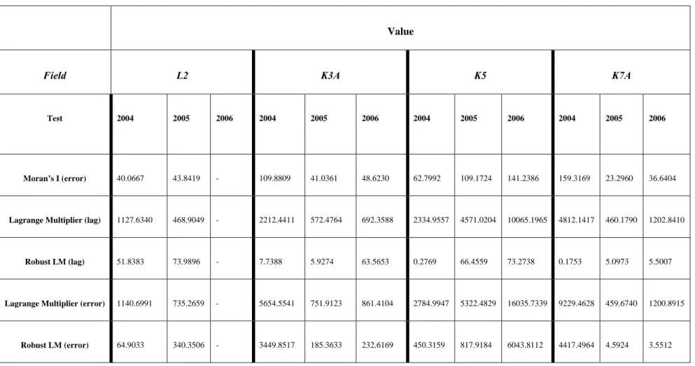
Spatial autocorrelation was also expected in this type of data and the SER model was estimated to detect it. The spatial model was more appropriate for analysis so that the spatial effects could be taken into account. However, the OLS regression test had to be conducted in order to determine which spatial regression model (lag or error) would be most appropriate. Five diagnostic tests for spatial dependence are reported with the OLS regression output in GeoDaTM and these include the Moran’s I for the spatial error model and the Lagrange Multiplier (LM) and its Robust for the lag and error models. In Table 2 there is a summary of the results for the five diagnostic tests for each field over the three years.
TABLE 2: DIAGNOSTIC TESTS FOR SPATIAL DEPENDENCE
Value
Field L2 K3A K5 K7A
Test 2004 2005 2006 2004 2005 2006 2004 2005 2006 2004 2005 2006
Moran’s I (error) 40.0667 43.8419 - 109.8809 41.0361 48.6230 62.7992 109.1724 141.2386 159.3169 23.2960 36.6404
Lagrange Multiplier (lag) 1127.6340 468.9049 - 2212.4411 572.4764 692.3588 2334.9557 4571.0204 10065.1965 4812.1417 460.1790 1202.8410
Robust LM (lag) 51.8383 73.9896 - 7.7388 5.9274 63.5653 0.2769 66.4559 73.2738 0.1753 5.0973 5.5007
Lagrange Multiplier (error) 1140.6991 735.2659 - 5654.5541 751.9123 861.4104 2784.9947 5322.4829 16035.7339 9229.4628 459.6740 1200.8915
The model with the highest Lagrange Multiplier (LM) value and its robust term is the most appropriate (Table 2). The spatial error model appears to be the most appropriate for 2004, 2005 and 2006 for fields L2, K3A and K5. In the 2005 and 2006 production years, the spatial lag model is more appropriate for K7A.
5.3 REML geo-statistic approach
When spatial correlation is present, field heterogeneity may be underestimated. The inferences about crop response to VRT may be misleading. Spatial regression techniques are necessary, because the data obtained from agronomic experiments are almost always spatially correlated. The restricted maximum-likelihood (REML) technique is one of the most common spatial regression techniques used (Bullock & Lowenberg-DeBoer, 2007). The REML-geostatistical approach was introduced by Cressie in 1993. This approach is often used to analyse yield monitor data and the semi-variogram is the backbone of this approach (Lambert, Lowenberg-DeBoer & Bongiovanni, 2004).
In yield monitor data and other spatial data, there is often correlation among neighbouring observations and this violates the assumptions of classical statistical analysis. From the viewpoint of classical agronomic research, this correlation makes the analysis of this type of data rather difficult and invalid. The reason is that the ignorance of spatial structure results in variance estimates that tend to be inflated. This means that significant levels of test statistics therefore tend to decrease which results in unreliable statistical inference. The under-estimation of heterogeneity and inefficient or biased inferences can result in imprecise inferences about the profitability analysis of trials comparing VR to SR application rates of P (Maine, 2006).
5.4 Model selection for spatial differences (regression)
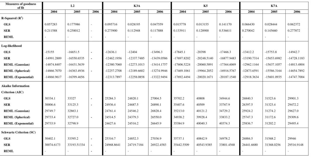
In ordinary regression analysis, the R-squared (also called coefficient of determination) is usually used as a measure of goodness of fit, with the model with the highest R-squared considered having the best fit and this implies that the predicted values match the observed values for the dependent variable. R-squared increases in value with
additional explanatory variables and over-fitting can occur. In Table 3, a summary of the goodness of fit is presented.
TABLE 3: MODEL SELECTION FOR SPATIAL DIFFERENCES
Measures of goodness
of fit L2 K3A K5 K7A
2004 2005 2006 2004 2005 2006 2004 2005 2006 2004 2005 2006 R-Squared (R2 ) OLS SER REML 0.057283 0.211588 - 0.177986 0.258012 - - - - 0.095716 0.273900 - 0.028195 0.112948 - 0.047559 0.117888 - 0.015778 0.133911 - 0.013155 0.128900 - 0.141170 0.536611 - 0.066430 0.270042 - 0.028444 0.145660 - 0.062372 0.277872 - Log-likelihood OLS SER REML (Gaussian) REML (Spherical) REML (Exponential) -15155 -14991.2889 -14874.8407 -14866.7070 -14866.9617 -16651.5 -16550.6535 -16431.5639 -16363.4936 -16399.4656 - - - -12636.1 -12462.1956 -12380.7060 -12257.2708 -12313.7897 -12404 -12337.7485 -12273.1013 -12189.6602 -12258.0858 -13496.3 -13439.0586 -13414.1757 -13274.9946 -13322.9494 -17845.1 -17697.8202 -17606.5224 -17469.1061 -17692.4494 -20398 -20248.5140 -20060.5891 -19964.2052 -20020.1671 -17466.3 -16877.9483 -17364.6069 -16916.5767 -20187.1540 -13412.2 -13190.7314 -12962.1164 -12873.6591 -12918.3634 -15753.8 -15653.6982 -15637.1057 -15586.3164 -15601.0935 -14942.7 -14728.1183 -14813.4804 -14654.7892 -14747.7004 Akaike Information Criterion (AIC) OLS SER REML (Gaussian) REML (Spherical) REML (Exponential) 30334.1 30006.6 29749.7 29733.4 29733.9 33327 33125.3 32863.1 32727.0 32798.9 - - - 25284.3 24936.4 24761.4 24514.5 24627.6 24820.1 24687.5 24546.2 24379.3 24516.2 27004.5 26890.1 26828.4 26550.0 26645.9 35702.2 35407.6 35213.0 34938.2 35384.9 40808 40509 40121.2 39928.4 40040.3 34944.6 33767.9 34729.2 33833.2 40374.3 26840.3 26397.5 25924.2 25747.3 25836.7 31523.6 31323.4 31274.2 31172.6 31202.2 29901.3 29472.2 29627.0 29309.6 29495.4 Schwartz Criterion (SC) OLS SER REML 30402.1 30074.6173 - 33395.2 33193.51334 - - - - 25316.7 24968.8641 - 24852.3 24719.7184 - 27036.9 26922.4583 - 35737.1 35442.5509 - 40842.9 40543.9385 - 34978.2 33801.4568 - 26884.5 26441.6680 - 31568.2 31368.0256 - 29946 29516.9148 -
In Table 3 the R-squared is higher in the SER model for each of the four fields during each of the three years. The goodness of fit of the model cannot be based on R-squared alone, as it does not indicate whether the estimated partial regression coefficients are statistically different from zero (LeSage, 1998). R-squared is also not appropriate as a measure of fit in comparing spatial regression models. The Log-likelihood models become more reliable and these values measure how good or poorly the model predicts the output in the observed data. The model with the highest log-likelihood has the best fit. Table 3 indicates that the REML (spherical) model has the highest log-likelihood (less negative) values. However, the log-likelihood increases with additional variables, as does the R-squared, over-fitting the model. This over-fitting can be corrected by employing the Akaike Information Criteria (AIC) (Maine, 2006). The AIC value assigned to a model is only meant to rank competing models and tell which is the best among the given alternatives, (the lower the AIC value, the better the model) (Acquah, 2009). The absolute values of the AIC for different models have no meaning. The REML (spherical) model has the lower AIC values for each of the four fields during each of the three years. 6. Conclusion
There are significant differences to be observed between the results obtained with the OLS, SER and REML models (Table 3) and this may have an impact on decision-making. This fact, once again emphasises the importance of taking spatial effects into account. Methodologies not taking these effects into account and thus ignoring spatial dependencies of yield monitor data can cause inaccurate results and conclusions. All the measures of goodness of fit indicated an increase in fit from the OLS to the SER model, with the best fit being achieved with the REML model, implying that the use of this model resulted in more accurate estimates. The results for model selection for spatial differences (regression) indicate the following:
The R-squared was higher in the SER model for each of the four fields during the three years under review.
The REML model also produced lower Akaike Information Criteria (AIC) values in each of the four fields during the three years under review.
The following conclusion was generated in hypothesis testing: spatial econometric models resulted in more accurate estimates than those achieved with the OLS models.
Bibliography
Acquah, H. D., Comaparison of Akaike information criterion (AIC) and Bayesian information criterion (BIC) in selection of an asymmetric price relationship. Department of Agricultural Economics and Extension, University of Cape Coast, Cape Coast, Ghana. E-mail: [email protected]. Journal of Development Agricultural
Economics, 2(1):001-006.
Anselin, L., Bongiovanni, R. & Lowenberg-DeBoer, J. 2004. A spatial econometric approach to the economics of site-specific nitrogen management in corn production.
American Journal Agricultural Economics, 86(3):675-687.
Auernhammer, H. 2002. The role of mechatronics in crop product traceability.
Agricultural Engineering International: The CIGR Journal of Scientific Research and Development. Invited overview paper. Vol. 4. October, 2002. Presented at the club of Bologna meeting, July 27, 2002. Chicago, IL., USA.
Bullock, D. S. & Lowenberg-DeBoer, J. 2007. Using spatial analysis to study the values of variable rate technology and information. Journal of Agricultural Economics, 58(3):517-535. 2007.
Florida Institute of Phosphate Research. 2004. Phosphate and organic fertilization,
History of phosphate fertilizer production and Introduction: phosphate as an essential mineral [online]. Available from: http://www1.fipr.state.fl.us/Phosphate [Accessed 12 March 2008].
Gandonou, J., Stombaugh, T. S., Dillon, C. R. & Shearer, S. A. 2001. Precision
agriculture: A break-even acreage analysis [Paper Number: 01-1029]. The Society for Engineering in Agricultural, Food and Biological Systems, Sacramento Convention Center, Sacramento, California, USA, 30 July – 1 August 2001. Written for presentation at the 2001 American Society of Agricultural Engineers Annual (ASAE) internationally meeting.
Griffin, T. W., Brown, J. P. & Lowenberg-DeBoer, J. 2005. Yield monitor data analysis:
Data acquisition, management and analysis protocol [Version 1, August 2005]. Department of Agricultural Economics, Purdue University.
Griffin, T. W. & Lowenberg-DeBoer, J. 2008. Spatial analysis of precision agriculture
data: Role of extension. Selected paper presented at the Southern Agricultural Economics Association Annual Meeting, Dallas, TX, February 2-6, 2008.
Khanna, M., Epouhe, O. F. & Hornbaker, R. 1999. Site-specific crop management: Adoption patterns and incentives.Review of Agricultural Economics, 21(2):455-472. Lambert, D. M., Lowenberg-DeBoer, J. & Bongiovanni, R. 2003. Spatial regression
models for yield monitor data: A case study from Argentina. Paper presented at the American Agricultural Economics Association Annual Meeting, Montreal, Canada, July 27-30, 2003.
LeSage, J. P. 1998. Spatial econometrics. MATLAB Guide. Department of Economics, University of Toledo.
Maine, N. 2006. The profitability of precision agriculture in the Bothaville district. Ph.D. thesis, Department of Agricultural Economics (Agricultural Management), Faculty of Natural and Agricultural Sciences, University of the Free State, Bloemfontein, South Africa.
Nell, W. T., Maine, N. & Basson, P. M. 2006. Africa, Part III: Current status: In: A. Srinivasan (Ed.), Handbook of precision agriculture: Principles and applications. New York: Food Products Press, Chapter 17:465-500.
Roberts, R. K., English, B. C. & Larson, J. A. 2002. Factors affecting the location of precision farming technology adoption in Tennessee [online]. Journal of Extension, 10(1). Available from: http://www.joe.org/joe/2002/february/rb3.html [Accessed 26 June 2003].
Robinson, E. 2005. Variable-rate phosphate helps rice [online]. Delta Farm Press. Available from:
http://www.printthis.clickability.com/pt/cpt?action=cpt&title=Variable-rate+phosphate [Accessed 25 February 2005].
Sadler, E. J., Jones, J. W. & Sudduth, K. A. 2007. Modeling for precision agriculture: how good is good enough, and how can we tell? Precision Agriculture, ’07:241-248. United States Department of Agriculture (USDA) – Agriculture Research Service (ARS), Columbia, MO 65211. University of Florida, Ganiesville, FL 32611. United States of America.
Snyder, C., Schroeder, T., Havlin, J. & Kluitenberg, G. 1996. An economic analysis of variable rate nitrogen management. Proceedings of the Third International Conference
on Precision Agriculture, June 23-26, 1996. Minneapolis, Minnesota.
Swinton, S. M. & Lowenberg-DeBoer, J. 1998. Profitabiltiy of site-specific farming.
Site-specific management guidelines. SSMG-3. Published by the potash and phosphate institute (PPI). Coordinated by South Dakota State University (SDSU).