Centro de
Investigación
Operativa
I-2008-3
WISCHE: A decision support
system for water irrigation
scheduling
M. Almiñana, L.F. Escudero, M. Landete,
J.F. Monge and J. Sánchez-Soriano
May 2008
ISSN 1576-7264
Depósito legal A-646-2000
Centro de Investigación Operativa
Universidad Miguel Hernández de Elche Avda. de la Universidad s/nWISCHE: A decision support system for water irrigation
scheduling
1
M. Almi˜nana1, L.F. Escudero2, M. Landete1, J.F. Monge1 and J. S´anchez-Soriano1
1 Centro de Investigaci´on Operativa
Universidad Miguel Hern´andez, Elche (Alicante), Spain e-mail: {marc,landete,monge,joaquin}@umh.es
2 Departamento de Estad´ıstica e I. Operativa
Universidad Rey Juan Carlos, Madrid, Spain e-mail: laureano.escudero@urjc.es
April 28, 2008
Abstract
In this paper we describe software and algorithms which are being used as a decision support system (DSS) tool to determine water irrigation scheduling. The DSS provides dynamic planning of the daily irrigation scheduling for a given land area by taking into account the irrigation network topology, the water flow technical conditions and the logistical operations. The system has been validated by the technicians of the Agriculture Community of Elche and incorporated into their Supervisory Control and Data Acquisition system (SCADA). We present two approaches to solve the mixed 0-1 separable nonlinear program for irrigation scheduling implemented with free software.
Keywords: water resource scheduling, agricultural irrigation, mixed 0-1 separable nonlinear program.
1
Introduction
In 1968 the Council of Europe published the European Water Charter (http://assembly.coe.int/), which states fundamental principles for the consevation of water resources and establishes criteria for their rational use. Besides outlining the fundamental principles for the protection of this indispensable and vital asset, the European Water Charter points out the need for the inventory, control and management of water resources.
The need for rational water management has become greater in many Mediterranean regions as a result of changes in the availability of water, changes in general climatic conditions and the adverse effect of the actions of human beings on the evironment. See [4] and the references therein for more details of water-related problems in Mediterranean regions.
Over the last years the traditional irrigation scheduling systems have been changed for other new systems in the southeast of Spain because of the scarcity of water resources in this arid Spanish region. The traditional inundating irrigation systems have been progressively substi-tuted by drop (sprinkler) irrigation systems, in which the water is channeled to the irrigation
1
This research has been partially supported by the grants from the Spanish Ministry of Education and Science and FEDER funds through the grant MTM2004-01095.
points where it is necessary and the required quantity is completely regulated and controlled. This kind of irrigation systems is more common day by day in the above mentioned region.
The ability to help the decision maker in the planning and distribution scheduling of the water resource systems depends on the level of sophistication of the tools and techniques avail-able. A comprehensive approach may remedy the inadequacies of the tools currently available, by developing a hydrologic modelling framework and a highly numeric intensive computation decision support system. See [7, 8, 9, 10, 12] and the references therein.
We should differentiate between water resource planning over a time horizon which is usually long and water distribution scheduling which is usually on a daily basis. For the case of planning see [2] for the deterministic environment, and [6, 11] for the stochastic case by considering the uncertainty in the main parameters (water inflow and needs).
The Agriculture Community of Elche (ACE), Elche being a city in the southeast of Spain, belongs to a group of people who are constantly looking for new irrigation systems in order to conserve the natural environment and to save as much water as possible, because they realize the future of the region depends in some way on the management of the scarce and important resource which water is. At this moment, the ACE is in a first phase of modernization of the channelling systems and the distribution of irrigation water among its members. The first phase in this work was the substitution of the water canalization for a new system consisting of underground pipes and pumps. The pumps send the water from the dam to each irrigation area. The system is controlled by means of a SCADA (Supervisory Control and Data Acquisition) which controls and regulates the available flow in each irrigation area. The advantages of this improvement to the installations are obvious. On the one hand, the water lost by evaporation and filtering is reduced and, on the other hand, each member of the ACE has the guarantee of a fixed quantity of irrigation water with a specific pressure on his land.
This improvement in the infrastructures of the irrigation system is very important in order to save irrigation water but there are two technical problems to be resolved; (i) the design of the pipe network does not guarantee the irrigation service to all members of the ACE simultaneously, therefore some priority criteria are needed in the management of the system.; (ii) the overall pressure of the pipe network has to be controlled to avoid possible breakage of the pipes or water losses. To determine the irrigation scheduling we have considered a set of time periods. In each period the members of the ACE are divided into two groups: active and non-active. Each member of the active group has a certain water flow volume and a minimum pressure in that period of time guaranteed and each member of the non-active group has the service of the irrigation water blocked. The SCADA controls the opening and closing of the valves.
The DSS WISCHE (Water Irrigation for SCHEduling) provides a solution to the problem of assigning each member of the ACE to a period of time in the daily irrigation scheduling, such that the flow and the minimum service pressure are guaranteed. In addition, the solution provided guarantees that the water flow speed in the network does not exceed a previously fixed maximum value.
As the preferences of the members of the ACE over all daily periods could be the same or coincide in some periods and, very likely, it is impossible to satisfy all preferences simultaneously, a special module has been incorporated into the system which records the past consumption of water and preferences for each hydrant. Thus, we are able to determine indices of efficient use and the service times. These indices allow us to determine a priority of use for each member of the ACE. The optimization model implemented in the software maximizes the number of members served according to their preferences weighted by their priority indices. A more detailed description of the problem can be found in [1], where a mixed zero-one separable non-linear model for the water irrigation scheduling is presented; it is solved by successively optimizing mixed 0–1
User Administrator WISCHE SCADA input data report s scheduling telemetry con trol
Figure 1: Components of the decision support system and flow of data
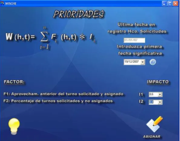
Figure 2: Control Panel
linear programs.
For a good exposition of mixed 0–1 linear programming, see e.g. [13], and see [3] for a mixed-integer linear programming in a irrigation scheduling problem in another context . The decision support system presented in this work has been tested by for solving a real-life problem presented by “La Comunidad de Regantes, Riegos de Levante, Canal 2nd”, which belong to ACE. Its irrigation area comprises 2188 Has and is distributed in 20 pipe sectors (i.e., 20 head nodes) with a total number of 2831 nodes (2025 of them are hydrants with their own water demand needs). The irrigation is needed on a daily basis for a set of time periods. The water flows from a reservoir with a capacity of 13Hm3, and the full system has an arborescent structure.
The remainder of the paper is organized as follows. In Section 2 we describe the structure of the decision support system WISCHE. Section 3 is devoted to describing the priority system for the hydrants. In Section 4 we present the optimization models implemented in the software WISCHE. Finally, Section 5 concludes.
2
WISCHE structure
WISCHE is a decision support system connected to the a SCADA. It sends to the control system the weekly planning of the irrigation system, providing information about which hydrant users will be served in each period, and receives information from the control system on the water consumption of each hydrant. A scheme illustrating the implemented systems and the relation between them is shown in Figure 1.
Figure 3: Graphics Form
Figure 4: Turns Form
module is Telemetr´ıa (Telemetry) and it processes historical data of telemetry, debugs reading errors and provides tools to create graphs of water consumption, pressure, etc. Figure 3 shows a graph illustrating minimum and maximum pressures of a set of hydrants generated from the telemetry data obtained during a period of 5 days. The second module, called Asignaci´on de Prioridades (Priorities’ Assignment), allows to introduce the periods preferred by each hydrant user, see Figure 4. Additionally it allows to modify the priority criteria, see Figure 5. Finally, the planning and assignment module provides the optimal assignment of irrigation periods to each member of the ACE. The diagram shown in Figure 6 describes the structure of the files that the three modules of WISCHE and the SCADA share among each other. The modulePriorities’ Assignment is responsible for processing all the information in the file telemetry, together with the history of the members preferences and their new preferences for the following week. Taking into account all this information, the module generates a set of priorities for each hydrant user and time period. This set of priorities is used by the optimization module. The optimization module will be described in Section 4.
The Priorities’ Assignment module is in charge of processing the information from the telemetry file, jointly with the file of past requests and the current preferences of the users for the next weekly planning. It generates a set of priorities for each hydrant user and time period
Figure 5: Priorities’ Assigment Form WISCHE history request file TELEMETRY REQUEST SCHEDULING APPROACH telemetry file topology file request file SCADA
Figure 7: Generating irrigation time periods form
to be used by the optimization module. The components of this module, see Figure 7, are described in section 4.
3
Hydrant priorities
As it is probably impossible to satisfy the preferences of all the members of the ACE because of the design and dimension of the irrigation network and the constraints on the pressure and the speed of the water, it is absolutely necessary to have a mechanism which prioritizes the assignment of a particular hydrant to a period of irrigation when there are several hydrants with the same or coincident preferences.
ThePriorities’s Assigmenment module of WISCHE receives the preferences of the members of the ACE in a table-form (see Figure 4). These preferences are then combined with the past history of use of the hydrant. We have taken into account two significant factors to determine the assignment of a hydrant to a particular irrigation period:
• Factor 1: Efficiency in the use of the preferred assigned periods in a number of previous weekly plannings.
• Factor 2: Percentage of preferred periods and not assigned in a number of previous weekly plannings.
Both factors provide two indices (in [0,1]) which measure, for each hydrant user, the efficiency in the use of the preferred irrigation period (Factor 1) and the percentage of times that their preferred periods have not been assigned (Factor 2). These factors are used in the system to calculate the users’ weights in the assignment of the irrigation scheduling, i.e., the weightW(t, h) being evaluated as an adjusted average of both factors, average adjusted by an impact value of each factor. The software allows to modify the impact that both indices will have in the weight assigned to the hydrants for each irrigation period. The priority of hydrant h for the irrigation time period tis computed as follows:
P(h, t) = W(h, t)
|t−t0|+ 1
whereW(h, t) is the weight assigned to hydrant h for the irrigation time periodt, andt0 is the
4
Optimization Models
The optimization module (Figure 7) needs four parameters, namely, number of irrigation time periods, maximum speed of the water flow, minimum pressure and pressure in the head hydrants. See Appendix A for more details on all these parameters. This module allows for the optimization of three models with two different approaches.
4.1 Models
M P F−ISP: Maximize the priority factor in the irrigation scheduling problem. In Appendix
A.1 we provide a description of a mixed zero-one separable non-linear problem for the irrigation scheduling. See in [1] the solution aproach that we have proposed.
M M−S: Minimize the Maximum Speed in the whole network. See Appendix A.2 for a
descrip-tion of this model.
M M−P Minimize the Maximum Pressure in the whole network. See Appendix A.3 for a
de-scription of this model.
We present two approaches to solve the model:
• Optimization approach using the free GLPK library: Approximated procedure to solve the quadratic mixed 0-1 model of irrigation planning.
• Heuristic approach: Heuristic algorithm to find a feasible solution in a relatively short time.
Depending on the characteristics of the instance, M P F−ISP can be non-feasible. In this
case the modification of certain constraints in the system could be required, either the minimum pressure or the maximum speed of the water. The user can compute the minimum maximum-speed of the system with all other parameters fixed, so he can adapt the maximum maximum-speed parameter to obtain a feasible value for the instance in hand. For example, the default maximum value in the system is 2.5 m/s. This maximum speed is feasible in the whole system provided the irrigation planning for the 2831 hydrants is in 5 periods per day. If the user of the control system makes the decision to offer only 3 irrigation periods per day, but, simultaneously, wants to provide an irrigation service to the 2831 hydrants, then he should modify the maximum speed constraint to obtain feasible solutions to the planning problem. Next he can compute the minimum maximum speed required by the system; in our particular case, there are points in the system where the water flow speed is 3.68 m/s. Then, he can solve the irrigation planning problem with only 3 periods per day fixing the maximum speed at a value above 3.68 m/s.
The running times for each optimization approach are shown in Table 2, for a real-life instance whose dimensions are given in Table 1 and the headings are as follows: m, number of constraints; nc, number of continuous variables; n01, number of 0-1 variables; nel, number of
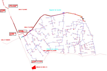
nonzero elements in the constraint matrix; anddens, matrix density. Notice the large dimensions of the separable nonlinear model. See in Figure 8 the instance’s topography.
4.2 Optimization approach using library GLPK
We have implemented the algorithm described in [1] over a windows platform with the free software GLPK (see, http://www.gnu.org/software/glpk/). Due to the complexity of the model
Table 1: Model Dimensions m 44390 nc 14155 n01 9848 nel 332231 dens 0.031 %
Table 2: Computing effort for different optimization approaches
Optimization model machine processor memory Obj. value time GAP
M P F−ISP (CPLEX approach) SUN W2100 Opteron 2.6 GHz 4 Gb 97346 2 min
-M P F−ISP (GLPK base heuristic) PC Pentium 1.6 GHz 2 Gb 97308 40 min 0.04 %
M P F−ISP (heuristic approach) PC Pentium 1.6 GHz 2 Gb 90159 1.5 min 4.7 %
M M−S (GLPK based heuristic) PC Pentium 1.6 GHz 2 Gb 2.211 m/s 40 sec.
M M−P (GLPK based heuristic) PC Pentium 1.6 GHz 2 Gb 68.53 mca 4 sec.
M P F−ISP the optimization engine GLPK did not provide the results in the affordable
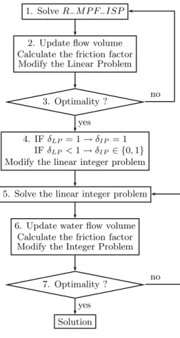
com-putation time, therefore, we developed a GLPK- based heuristic procedure in order to solve the problem. It can be summarized as shown in the following 6 steps:
1. Solve the approximate linear relaxation (R−M P F−ISP) of the continuous model of the
irrigation scheduling problem (M P F−ISP), where the linear Taylor series expansion
ap-proximation of the quadratic variables is used and the 0-1 variables are relaxed to contin-uous variables. We use the GLPK library.
2. Update the water flow volumes for the obtained solution.
3. If the linear solution is a solution for the quadratic continuous problem, then we go to the next step. Otherwise, we update the approximation point of the Taylor series to the quadratic model and go to step 1.
4. Fix the relaxed 0-1 δ variables with value 1 in the solution of the linear relaxation. 5. Solve the linear integer approximation of the integer quadratic problem only taking as 0-1
variables those with a fraction value in the previous step.
6. If the integer solution is a solution of the quadratic integer problem, then we stop. Oth-erwise, we update the approximation point to the quadratic model and go to step 4. The flow diagram of the the algorithm is shown in Figure 9.
The optimality GAP is 0-04% (see table 2), what is very good but the elapsed time is 40 minutes. This time is valid for planning and simulation studies but is not affordable for scheduling work. The modelsM MS and M MP are optimized by using the same GLPK-based procedure.
4.3 Heuristic approach
For scheduling work we have implemented a faster heuristic algorithm to obtain a quasi-optimum solution in an affordable computational time.
Figure 8: Instance topography
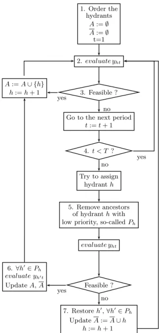
1. Order the hydrants by the non-increasing valuepriority/water-flow-volume. Let A be the set of hydrants provisionally assigned to an irrigation period, and let ¯A be the set of non-yet assigned hydrants in the algorithm.
2. For hydrant h with highest priority for the irrigation time period t, call the function
evaluateyht. This function updates the water flow volume from hydrant h to its head
node analyzing whether it is feasible to assign hydrant h to the irrigation time periodt, i.e., whether the pressure and speed constraints are satisfied along the path from hydrant
h to its head node.
3. If hydrant h can irrigate during time periodt, then we update set A and go to step 2. 4. If there are still irrigation time periods to assign to hydrant h, then increase t and go to
step 2.
5. Remove the hydrants which are ancestors of hydrant h and have less priority than it, such that their accumulate water flow volumes exceed the water flow volume required by hydranth. Let us callPh to this set of hydrants. In such a case the assignment of hydrant
h to its maximum priority irrigation time period is feasible.
6. If hydrant h can be assigned to the irrigation time period t, then we try to assign the previously removed hydrants included in set Ph, update the sets A and ¯A and go to step
2.
7. Otherwise, restore the removed hydrants of Ph and, again, update the setsA and ¯A.
Note: If after a complete iteration of the algorithm the set of non-assigned hydrants ¯A is nonempty, then again run the algorithm given priority to these nodes.
The flow diagram of the algorithm is shown in Figure 10.
Table 2 shows the time (1.5 minutes) and the optimality GAP (4.7%) of the heuristic, what is fully affordable for scheduling work.
1. SolveR−M P F−ISP
2. Update flow volume Calculate the friction factor Modify the Linear Problem
3. Optimality ?
4. IFδLP= 1→δIP = 1
IFδLP <1→δIP ∈ {0,1}
Modify the linear integer problem
5. Solve the linear integer problem
6. Update water flow volume Calculate the friction factor Modify the Integer Problem
7. Optimality ? Solution yes yes no no
Figure 9: Optimization approach
4.4 Computational results
In this section we show different solutions of the algorithms by varying the number of irrigation time periods. The computational experience was executed on an Intel Core Duo 1.66 GHz. pro-cessor, with 2 GB. RAM running under Micrososft Windows XP operating System. Note that the network only can satisfy the water demand for all the hydrants when 5 or 6 time periods are considered. For less than 5 periods we need to minimize the maximum pressure to obtain a feasible water flow speed in the network. Table 3 shows the solution for the M P F−ISP model
using WISCHE. The headings are as follows: nper, is the number of periods in daily planning,
ZGLP K and ZH provide the solution value using the GLPK-based heuristic and Heuristic
ap-proaches respectiely, Vmax is the solution of theM M−S problem, this solution is the maximum
water flow speed allowed for the scheduling problem, except for Vmax = 2.5m/s since it is the
default value. Notice that the Heuristic solution does not differ from the optimal solution in more than GAP = 11%, where GAP = (ZH −ZGLP K)/ZGLP K and on the other hand the
elapsed time is very affordable.
5
Conclusions
WISCHE is an application built jointly with Riegos de Levante (the main group from the Agri-culture Community of Elche, ACE), irrigation community which has a real need for irrigation
1. Order the hydrants A:=∅ A:=∅ t=1 2. evaluate yht A:=A∪ {h} h:=h+ 1 3. Feasible ?
Go to the next period
t:=t+ 1 4. t < T ? Try to assign hydranth 5. Remove ancestors of hydranthwith low priority, so-calledPh
evaluate yht 6. ∀h′∈P h evaluate yh′t UpdateA,A Feasible ? 7. Restoreh′,∀h′∈P h UpdateA:=A∪h h:=h+ 1 yes no no yes yes no
Table 3: Computational effort for different planing daily basis nper GLP K time Heuristic time GAP (%) Vmax
1 107.895 1 sec. 107.895 1 sec. 0.0 8.87 m/s 1 infeasible - infeasible - - 2.5m/s 2 115966 25 sec. 114.552 15 sec. 1.2 5.30 m/s 2 infeasible - infeasible - - 2.5m/s 3 108.577 2 min. 104.914 35 sec. 3.3 3.70 m/s 3 infeasible - infeasible - - 2.5m/s 4 100.527 20 min 93.392 40 sec. 7.1 2.78 m/s 4 infeasible - infeasible - - 2.5m/s 5 92.900 35 min 83.932 90 sec. 9.9 2.23 m/s 5 97308 60 min 90.158 90 sec. 7.3 2.5m/s 6 86.555 72 min 77.805 80 sec. 10.1 1.84 m/s 6 97.489 48 min 93.476 8 sec. 4.1 2.5m/s
scheduling because water demand usually exceed water availability. This software allows irri-gation community managers to schedule hydrant turns one week in advance. Scheduling is as flexible as possible and the priority system presented allows for all farmers to be seviced accord-ing to their previous usage, so farmers who make early applications and usually make reasonable use of their demand benefit from the proposed support system.
Appendix
A
Mathematical Models for irrigation scheduling
In order to describe mathematically the irrigation scheduling problem, we need to take into account technical, topographical and logistic irrigation scheduling parameters. The technical and topographical parameters are related to the physic properties of the fluids. The logistic parameters are related to the management of the irrigation system and, finally the irrigation scheduling parameters are related to constraints in the way of assigning the irrigation time periods. Finally, the decision variables are related to the water volume of flow though each node at each time period and to when each hydrant may sink down.
The notation for all relevant elements and parameters in the WISCHE system is the following:
Sets of general elements:
T, set of time periods for water irrigation purposes.
I, set of hydrants and bifurcation nodes in the geographical area under consideration.
I0, set of bifurcation nodes.
Iτ ⊂ I −I
0, subset of hydrants whose irrigation starting period has already been fixed to time
periodτ,τ ∈ T.
Γ, set of sector heads, and γ(i) ∈ Γ is the root node (sector head) of the subtree to which hydrant ibelongs.
Ri, set of upstream nodes to hydranti, in its path back to its sector head, including the same
hydrant i, fori∈ I −I0.
Si, set of successor nodes to nodei, including the same hydrant i, for i∈ I. Notice that the
nodes in setSican belong to different successor paths (this is the case where the successor
path has bifurcation nodes).
Technical and topographical parameters:
fit, friction factor for obtaining the pressure in the immediate upstream pipe segment of hydrant
iat time period t, to be updated iteratively, for i∈ I − I0, t∈ T. The friction factor can
be calculated by using the Colebrook-White equation (see e.g., [5]). The computation of
f will be iteratively performed each iteration of the algorithm for a given water discharge. Colebrook-White formula is a nonlinear equation in f, but we make use of the Newton-RAphson procedure to obtain its roots.
Ei, elevation of nodei, fori∈ I ∪Γ.
Li, length of the immediate upstream pipe segment of node i, for i∈ I ∪Γ. Di, diameter of the immediate upstream pipe segment of node i, fori∈ I ∪Γ.
g, gravity acceleration coefficient.
Hγ, pressure at sector head γ, for γ ∈Γ.
Hmin, minimum pressure required by any hydrant at any time period.
vmax, maximum water flow speed allowed along the immediate upstream pipe segment of any
K, hydromodule (l/s/ha), i.e., constant to obtain the water flow volume to irrigate the land area through any hydrant at any time period.
Irrigation scheduling parameters:
ˆ
Ni, duration (i.e., number of time periods) of the irrigation by hydrantibased on the dimensions
(has) of its respective land area, for i∈ I − I0.
Logistic parameters provided by the system operator:
cit, priority coefficient for selecting hydrantito begin a non-preempted irrigation at time period
t, for i∈ I − I0.
Fi, effective land area (has) to be irrigated by hydrant i, fori∈ I − I0.
ˆ
yiτ, fixed value to 0 or 1 for the variable yiτ due to logistic considerations, for i∈ Iτ. Variables:
qit, water discharge to flow through nodeiat time periodtto satisfy its own needs, if any, and
the water needs of its successor nodes, fort∈ T, i∈ I ∪Γ.
yit, 0–1 variable, such that its value is 1 if the irrigation in hydrant i begins at time period t
and, otherwise, it is zero, fort∈ T, i∈ I − I0. Notice that the irrigation is carried out in
periods t, . . . , t+ ˆNi−1 such thatyit= 1.
A.1 M P F−I SP: Mixed 0–1 separable nonlinear approach for water irrigation
scheduling
The mathematical expresion of the model for maximizing the priority factor in the irrigation scheduling problem (M P F−ISP) is as follows:
max X i∈I−I0 X t∈T cityit (1) s.t. Hγ(i)+Eγ(i)−Ei −P j∈Ri 8fjtLj π2gD5 j q2jt ≥Hmin ∀t∈ T, i∈ I − I0 (2) qit=Pj∈Si−I0−ΓKFj( P τ=t−Nˆj+1,...,tyjτ) ∀t∈ T, i∈ I ∪Γ (3) 4 πD2 i qit≤vmax ∀t∈ T, i∈ I ∪Γ (4) X t∈T yit= 1 ∀i∈ I − I0 (5) yit= ˆyit ∀i∈ Iτ, τ ∈ T (6) yit∈ {0,1} ∀t∈ T, i∈ I − I0 (7)
A.2 M M−S: Minimization of the maximum water speed
The model to minimize the maximum speed (M M−S) is as follows:
min Vmax (8) s.t. (2)−(3),(5)−(7) (9) 4 πD2 i qit≤Vmax ∀t∈ T, i∈ I ∪Γ (10)
where Vmax is the variable that gives the maximum water speed along the time horizon
A.3 M M−P: Minimization of the maximum water pressure
Another interesting objective function is the minimization of the maximum pressure of water in the irrigation network at any time period.
minP rmax (11) s.t.(2)−(7) (12) P rγ(i)+Eγ(i)−Ei−Pj∈Ri 8fjtLj π2gD5 j Q2jt ≤P rmax,∀i∈ I − I0, t∈ T (13)
where P rmax is the variable that gives the maximum water pressure along the time horizon.
.
References
[1] M. Almi˜nana, L.F. Escudero, M. Landete, J.F. Monge, A.Rabasa and J. S´anchez-Soriano. On a mixed 0–1 separable nonlinear approach for water irrigation scheduling. IIE Transactions 44(4) (2008), 398-405.
[2] J. Andreu, J. Capilla and E. Sanchis. AQUATOOL, a generalized decision-support system for water-resources planning and operational management. Journal of Hidrology177 (1996) 269–291. [3] A.A. Anwar and D. Clarke. Irrigation Scheduling Using Mixed-Integer Linear Programming.Journal
of Irrigation and Drainage Engineering127(2) (2001) 63–69.
[4] P. Balabanis, D. Peter, A. Ghazi and M. Tsogas, editors. Mediterranean desertification: Research Results and policy implementation, two volumes. European Commission, 2000.
[5] C.F. Colebrook. Turbulent flow in pipes, with particular reference to the transmition region between the smooth and rough pipe laws. Journal of the Institute of Civil Engineers11 (1938) 133–156. [6] L.F. Escudero. WARSYP, a robust approach for water resources planning under uncertainty.Annals
of Operations Research95 (2000) 313–339.
[7] J.W. Labadie, I.E. Brazil, I. Corbu and L.F. Johnson, editors. Computerized Decision Support
Systems for Water Managers. American Society of Civil Engineers, 1989.
[8] D.P. Loucks. Water resource systems models: their role in planning, Journal of Water Resource
Planning Management118 (1992).
[9] D.P. Loucks and J.R. da Costa, editors. Decision Support Systems. Water Resources Planning. Springer, 1991.
[10] J.B. Marco, R. Harboe and J.D. Salas, editors. Stochastic Hydrology and its Use in Water Resources
[11] M.V.F. Pereira and L.M.V.G. Pinto. Multistage stochastic optimization applied to energy planning.
Mathematical Programming52 (1991) 359–375.
[12] B. Recio, J. Iba˜nez, F. Rubio and J.A. Criado A decision support system for analysing the impact of water restriction policies. Decision Support Systems39 (2005) 385-402.