FACTORS INFLUENCING THE ECONOMIC PERFORMANCE OF A PANEL OF COMMERCIAL MILK PRODUCERS FROM EAST GRIQUALAND,
KWAZULU-NATAL, AND ALEXANDRIA, EASTERN CAPE, SOUTH AFRICA: 2007-2014
BY
JETHRO JAMES ROSS
Submitted in partial fulfilment of the requirements for the degree of
MASTER OF SCIENCE IN AGRICULTURE (AGRICULTURAL ECONOMICS)
in the
Discipline of Agricultural Economics
School of Agricultural, Earth and Environmental Sciences College of Agriculture, Engineering and Science
University of KwaZulu-Natal Pietermaritzburg
ii ABSTRACT
The South African dairy industry has been characterized, in recent years, by an observed movement towards fewer, larger producers, implying a more competitive milk market in which efficiency measures are likely to become increasingly important determinants of farm financial success and survival. Due to the imperfect nature of efficiency estimates, a more integrated approach is adopted in this study in which economic performance is defined as an unobservable variable for which there exist many imperfect indicators, including various measures of efficiency. This study presents a two-stage approach to analyse economic performance, and its key determinants, for a panel of commercial milk producers in East Griqualand (EG) and Alexandria, South Africa, over the period 2007-2014. Stochastic frontier analysis was used to estimate technical efficiency (TE) from a translogarithmic production function, selected ex-post from several specified models with different functional forms and distribution assumptions. Parametric scale efficiency (SE) was then estimated from the resulting scale elasticities and parameter estimates. Results indicate that sampled producers are, on average, highly technically efficient, generally operating close to the efficient frontier, and are relatively homogenous in production. The general decline of mean TE scores over the study period indicates that farms on the best practice frontier became more efficient over time, while the average farm has become less efficient in relation to the advancing frontier. High mean SE scores confirm that most farms do not experience a substantial loss in output due to scale efficiency problems, but rather to inefficiencies in production (TE). Analysis of SE scores reveals that most farms operated at suboptimal scale, with increasing returns to scale, and could improve output by expanding towards the optimal scale. Latent economic performance was modelled in a Multiple-Indicators, Multiple-Causes (MIMIC) model framework, with estimated TE and SE serving as imperfect indicators. Three latent indices were constructed to represent managerial quality regarding the breeding, feeding and labour programme, and were included in the structural equation, in conjunction with traditional explanatory variables, as latent causes of economic performance. Evaluation of model fit for several specified models led to the selection of the most simplistic specification, in which the latent managerial constructs were not included. Results suggest efficiency, milk yield per cow, and level of specialization in dairying all have a significant effect on the economic performance of the
iii
sampled farms. It should be noted that the sign of latent economic performance was not in line with expectations, and requires further research.
iv
DECLARATION
I, Jethro James Ross, declare that
1.1The research reported in this dissertation, except where otherwise stated, is my own original research.
1.2This dissertation has not been submitted for any degree or examination at any other tertiary institution.
1.3This dissertation does not contain other persons’ data, figures, graphs or other information, unless there is specific acknowledgement and appropriate reference to the source.
1.4This dissertation does not contain any other authors’ work, unless specifically acknowledged and appropriately referenced. Where other written works have been quoted:
a. The original words have been re-written, and the general information attributed to them has been appropriately cited.
b. Where their exact words have been used, their writing has been in quotation marks, and appropriately cited.
Signed:
16 March 2018
Jethro James Ross Date
I, as the main supervisor, agree to the examination of this dissertation:
16 March 2018
Professor Gerald Ortmann Date
v TABLE OF CONTENTS ABSTRACT ... ii DECLARATION... iv LIST OF TABLES ... ix LIST OF FIGURES ...x
LIST OF ABBREVIATIONS AND ACRONYMS ... xi
ACKNOWLEDGEMENTS ... xiv
CHAPTER 1: INTRODUCTION ...1
1.1 General introduction ...1
1.2 Objectives ...6
1.3 Importance of the study ...7
1.4 Structure of the dissertation ...9
CHAPTER 2: REVIEW OF PRODUCTIVITY AND EFFICIENCY ANALYSIS ...12
2.1 Introduction ...12
2.2 Productivity and the production function ...12
2.3 Measuring efficiency ...17
2.3.1. Parametric methods ...20
2.3.2. Nonparametric methods ...26
2.3.3. Semiparametric methods ...30
2.4 Flexible functional forms ...31
2.5 Technological change ...35
2.6 Productivity analysis in South Africa ...37
2.7 Concluding remarks ...39
CHAPTER 3: REVIEW OF LATENT VARIABLE ANALYSIS AND SEM TECHNIQUES ...41
3.1 Introduction ...41
vi
3.3 Structural equation modelling ...44
3.4 The MIMIC model ...45
CHAPTER 4: MILK PRODUCTION IN SOUTH AFRICA ...50
4.1 Introduction ...50
4.2 The South African dairy industry ...50
4.3 Dairying in KwaZulu-Natal ...56
4.4 Dairying in the Eastern Cape ...57
CHAPTER 5: MODELLING TECHNICAL AND SCALE EFFICIENCY ...58
5.1 Introduction ...58
5.2 Description of the study areas and the data collected ...58
5.2.1 Data ... 58
5.2.2 East Griqualand ... 59
5.2.3 Alexandria ... 63
5.3 Variables used in the production function ...67
5.4 Preliminary data analysis ...71
5.4.1 Missing data analysis ...71
5.4.2 Multiple imputation ...73
5.4.3 Multicollinearity analysis...73
5.4.4 Descriptive statistics ...75
5.5 Stochastic frontier analysis ...77
5.5.1 Cobb-Douglas production function ... 79
5.5.2 Simplified Translog production function ... 79
5.5.3 Translog production function ... 80
5.5.4 Generalized Leontief production function ... 81
5.5.5 Normalized Quadratic production function ... 81
5.5.6 Parametric scale efficiency ... 81
CHAPTER 6: EMPIRICAL RESULTS OF TECHNICAL AND SCALE EFFICIENCY ANALYSIS ... 84
vii
6.2 Choice of functional form and distributional assumption ... 84
6.3 Maximum likelihood results and discussion ... 88
6.3.1 Elasticity and parameter estimates ... 88
6.3.2 Technical efficiency ... 95
6.3.3 Scale efficiency ... 104
CHAPTER 7: MODELLING THE ECONOMIC PERFORMANCE OF DAIRY FARMS ...111
7.1 Introduction ...111
7.2 Variables used in the analysis of economic performance ...113
7.2.1 Structural equation variables...113
7.2.2 Measurement equation variables...116
7.3 MIMIC model specification ...117
7.4 Empirical results and discussion of the MIMIC model ...120
CONCLUSION ... 130
SUMMARY ... 134
REFERENCES ... 137
APPENDIX 1: MISSING DATA ANALYSIS ... 157
APPENDIX 2: MULTICOLINEARITY ... 159
2.1 Translog correlation matrix ...159
2.2 Condition index and variance decomposition for the Translog model ...160
2.3 Condition index and variance decomposition for the Cobb-Douglas model...160
APPENDIX 3: WITHIN MODEL LIKELIHOOD RATIO TESTS ... 161
APPENDIX 4: RESIDUAL PLOTS DEMONSTRATING GOODNESS OF FIT ... 164
4.1 Cobb-Douglas functional form ...164
4.2 Simplified Translog functional form ...164
4.3 Translog functional form ...165
viii
ix
LIST OF TABLES
Table 4.1: Geographical distribution of South African milk producers, 1997-2014 ...51
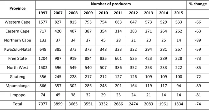
Table 4.2: Number of milk producers per province in South Africa, 1997 to 2015 ...53
Table 4.3: Mean herd size per producer, per province, for 2006 and 2014 ...54
Table 5.1: Variables included in the production function...68
Table 5.2: Descriptive statistics for the East Griqualand study group ...76
Table 5.3: Descriptive statistics for the Alexandria study group ...76
Table 6.1: Summary of modelled milk production technologies ...85
Table 6.2: Between-model likelihood ratio tests ...87
Table 6.3: Maximum likelihood estimates of the specified production functions, East Griqualand and Alexandria Dairy Farms, 2007-2014 ...89
Table 6.4: Descriptive statistics of mean technical efficiency per year, East Griqualand and Alexandria Dairy Farms, 2007-2014 ...96
Table 6.5: Frequency distribution of mean technical efficiency scores per farm size, and region, East Griqualand and Alexandria Dairy Farms, 2007 – 2014. ...103
Table 6.6: Descriptive statistics of mean scale efficiency per year, East Griqualand and Alexandria Dairy Farms, 2007 – 2014. ...105
Table 6.7: Efficiency scores and scale, East Griqualand and Alexandria Dairy Farms, 2007-2014. ...107
Table 6.8: Frequency distribution of mean scale efficiency scores per farm size, and region, East Griqualand and Alexandria Dairy Farms, 2007-2014. ...109
Table 7.1: Comparison of MIMIC model fit parameters ...122
x
LIST OF FIGURES
Figure 2.1: Single input-output production process ...13
Figure 2.2: Neoclassical three-stage production function and marginal and average curves ...16
Figure 2.3: Non-monotone production frontier ...32
Figure 3.1: A one-factor MIMIC model ...46
Figure 3.2: Path diagram for a multiple-factor MIMIC model ...48
Figure 5.1: Map of vegetation biomes in KwaZulu-Natal, South Africa ...60
Figure 5.2: Mean annual rainfall map for KwaZulu-Natal, South Africa ...61
Figure 5.3: Mean annual temperature map for KwaZulu-Natal, South Africa ...63
Figure 5.4: Map of vegetation biomes in the Eastern Cape, South Africa ...64
Figure 5.5: Mean annual rainfall map for the Eastern Cape, South Africa ...65
Figure 5.6: Mean annual temperature map for the Eastern Cape, South Africa ...66
xi
LIST OF ABBREVIATIONS AND ACRONYMS
GDP Gross Domestic Product
KZN KwaZulu-Natal
TFP Total Factor Productivity
GVA Gross Value Added
ROI Return on investment
ROE Return on equity
SEM Structural equation modelling
MIMIC Multiple Indicators, Multiple Causes
LAC Long run average cost
ISUR Iterative Seemingly Unrelated Regression FIML Full information maximum likelihood DEA Data envelopment analysis
TPP Total physical product
APP Average physical product
MPP Marginal physical product
TE Technical efficiency
AE Allocative efficiency
EE Economic efficiency
SE Scale efficiency
SFA Stochastic Frontier Analysis LCM Latent class model
xii
FDH Free Disposal Hull
CRS Constant returns to scale VRS Variable returns to scale NIRS Non-increasing returns to scale DGP Data generating process
LML Local maximum likelihood
RLb Richardson-Lucy blind deconvolution algorithm CNLS Convex nonparametric least squares
stoNED Stochastic non-smooth envelopment of data
MM Method of moments
GAM Generalized additive model EFA Exploratory factor analysis CFA Confirmatory factor analysis
ML Maximum likelihood
TMR Total mixed ration
KZNMPO KwaZulu-Natal Milk Producers’ Organisation
EG East Griqualand
EC Eastern Cape
BRG Bioresource Group
MCAR Missing completely at random
MAR Missing at random
MNAR Missing not at random
xiii TL Translog NQ Normalized Quadratic GL Generalized Leontief CD Cobb-Douglas STL Simplified translog TN Truncated normal HN Half normal
MPSS Most productive scale OLS Ordinary least squares
AI Artificial insemination
TLI Tucker Lewis Index
CFI Comparative Fit Index
RMSEA Root mean square error of approximation SRMR Standardized root mean square residual AIC Akaike information criterion
BIC Bayesian information criterion SSABIC Sample-size adjusted BIC
xiv
ACKNOWLEDGEMENTS
I would like to acknowledge and thank the following people for making this study possible: Professor Gerald Ortmann in the Discipline of Agricultural Economics, University of KwaZulu-Natal, for his guidance, encouragement, hard work, and patience during this study, and his funding assistance that made this study possible.
Mr Richard Bischoff, Agricultural consultant, Kokstad, for his willingness to provide data, advice, and assistance in making this study possible.
Mr Neil Currie, Agricultural consultant, Grahamstown, for his willingness to provide data, advice and assistance in making this study possible.
My family for their understanding, support, patience and encouragement throughout this study, and for providing me the opportunity to undertake this study.
Finally, Megan Ward for her constant support, encouragement, love and patience throughout this study and other difficult times.
1
CHAPTER 1: INTRODUCTION 1.1General Introduction
Agricultural production is an integral part of the national economy contributing R72.2 billion to GDP in 2015. Despite a decrease in agriculture’s share of GDP from 6% in the 1970’s to 2% in 2015 it remains an important sector of the national economy (Department of Agriculture, Forestry and Fisheries (DAFF), 2016). The South African dairy industry is the fifth largest agricultural industry in the sector, providing 60 000 jobs at the farm level and a further 40 000 indirect jobs in associated value chains, such as processing and milking (DAFF, 2014b). South Africa is currently a net exporter of dairy products, importing 40 199 tons and exporting 71 099 tons during 2015 (DAFF, 2015). In global terms, South Africa is a relatively small milk producing country, contributing just 0.5% of world milk production in 2014 (DAFF, 2014b).
Dairy industries in many countries have undergone significant structural change in the past two decades, with a consolidation trend towards fewer, larger milk producers. Melhim et al. (2009) highlighted the magnitude of these structural changes in the United States (US) dairy industry, reporting that between 1974 and 2002 the number of farms with milking cows declined by 79%. Furthermore, from 1964 to 2005 the number of milking cows per farm in the US increased by 60%. Evidence of industry consolidation can be found in several other studies on US milk producers (El-Osta & Morehart, 2000; Gloy et al., 2002; Tauer & Mishra, 2006; Gillespie et al., 2009; Hanson et al., 2013).
Evidence of significant structural change has also been found in other major milk producing countries such as New Zealand and Australia. Clark et al. (2007) found evidence of a consolidation trend in the New Zealand dairy industry, indicating that from 1994 to 2004 the number of cows on New Zealand dairy farms increased by 37%, while herd size increased by 63%. Kompas & Che (2003) reported a similar trend in the Australian dairy industry, reporting that between 1978-79 and 1999-2000 the number of dairy producers nearly halved. This large decrease in the number of dairy producers was, however, accompanied by almost a 70% increase in total milk production. This consolidation trend among Australian milk producers was further substantiated by Kompas & Che (2006). Furthermore, between 2001 and 2007, Hansson & Ferguson (2011) noted that the number of Swedish dairy farms decreased by 40%, while average herd size increased over the same period.
2
This observed movement towards fewer, larger producers is indicative of a more competitive milk market. In the face of increased competition, the economic efficiency of a milk producer’s operation is likely to become an increasingly important determinant of farm financial success (Weersink et al., 1990) and survival in the industry (Tauer & Belbase, 1987; Bravo-Ureta & Rieger, 1991).
There are several different measures of efficiency referenced in the literature, including technical, allocative, scale and economic efficiency. Technical efficiency may be defined as the ability of a firm to obtain maximum output from a given set of inputs (Farell, 1957). Scale efficiency measures the ray average productivity at the observed input scale relative to what is attainable at the most productive scale size (optimal scale) (Ray, 1998). In essence, this indicates how close the observed firm is to the optimal scale (Madau, 2011). Economic efficiency, which is the product of technical and allocative efficiency, refers to the ability of a firm to produce a predetermined quantity of output at minimum cost for a given level of technology (Farell, 1957). Economically efficient farmers utilize inputs to production effectively, producing output at lower cost for a given level of technology. This allows for improved profitability and a potential competitive advantage. In essence, commercial milk producers may be able to improve their competitive position in a highly competitive milk market through the exploitation of production advantages associated with improved levels of efficiency. In the long run, firms that are not technically efficiency will not survive, as the forces of competition will drive inefficient farms out of business (Tsionas, 2006). Investigating firm performance through the analysis of various measures of efficiency is commonplace in the literature although most studies consider only technical efficiency in their analyses. Likewise, farm performance has commonly been defined in terms of technical efficiency (Sedik et al., 1999; Diaz & Sanchez, 2008), although several studies have extended their scope to include allocative efficiency (Kalirajan & Shand, 2001) and economic efficiency (Hansson, 2007). Despite the continued popularity of efficiency measures in productivity analysis, it is important to highlight several possible limitations associated with their use as indicators of farm performance. Firstly, many definitions of efficiency exist, including economic, allocative, scale and technical efficiency (Coelli, 1995; Hansson, 2007). Secondly, there are various empirical techniques for the measurement of any one type of efficiency, the choice of which may have a significant effect on the estimated parameters and hence the validity of the results (Kalaitzandonakes & Dunn, 1995;
3
Balcombe et al., 2006; Bravo-Ureta et al., 2007). Finally, farm performance may be investigated using alternative measurement approaches, such as Total Factor Productivity (TFP) (Fraser & Hone, 2001; Fogarasi & Latruffe, 2009a) and Gross Value Added (GVA) (Thomassen et al., 2009; Giannakis & Bruggeman, 2015). TFP measures the overall efficiency of agricultural production and may be defined as the ratio of aggregate output to aggregate input (Pingali & Evenson, 2010; O’Donnell, 2010). Productivity growth therefore occurs when growth in output exceeds growth in inputs (Pingali & Evenson, 2010). GVA may be defined as the difference between the value of total production and non-factor costs, where non-factor costs may be defined as the total cost of all factors not directly attributable to the milk production process (Giannakis & Bruggeman, 2015). Given the imperfect nature of efficiency based performance analysis, it may be desirable to investigate the determinants of farm performance on a more integrated level, considering factors other than efficiency estimates. Investigating the economic performance of a farm, for instance, provides a means of identifying the critical factors that determine the success or failure of a farm. However, before proceeding with an analysis of economic performance, an unambiguous definition of the concept must be established. Economic performance is a concept lacking a concise definition among the literature although there is a general consensus that the definition depends upon the nature of the study and the aspect of performance that is to be investigated. Paul & Siegel (2006) consider economic performance as being based on the analysis of marketed inputs and outputs and define the concept in terms of productivity, technical efficiency and cost effectiveness. Lanoski (2000) identifies profitability measures, such as return on investment (ROI) and return on equity (ROE); growth, in terms of sales and market share, and firm financial success as common measures of economic performance. Although definitions of economic performance differ per their application, measures of productivity, financial success and growth are common themes among the literature. For the purposes of this study it is proposed that economic performance be defined as a latent, unobservable variable for which there exist many imperfect indicators, including various measures of efficiency (Richards & Jeffrey, 2000).
Defining economic performance as a latent (unobservable) variable requires that an appropriate latent variable modelling framework be specified. For the purposes of this study, a structural equation modelling (SEM) framework is used to model latent economic performance. More specifically, the Multiple-Indicators, Multiple-Causes (MIMIC) model, a special case of SEM, is
4
selected for its ability simultaneously to model the effects of various “cause” and “indicator” variables on latent economic performance. Within the MIMIC framework, efficiency estimates, included as “indicator variables”, and traditional observable “cause” variables such as herd size can be modelled simultaneously. The result is a comprehensive analysis of dairy farm economic performance, and its key determinants, at a level of integration not typically considered among the literature.
The rapid rate of consolidation identified in several important milk producing nations raises several important research questions, such as: 1) Do larger milk producers possess an inherent advantage over smaller producers, indicating the presence of size economies in the dairy industry? 2) In a highly competitive milk market, what strategies or factors are most important in improving economic performance and, hence, financial success? 3) Is technological variation between producers a significant determinant of farm performance and, therefore, a possible contributing factor to the consolidation trend? The answers to these questions could give commercial milk producers insight into which strategies or factors are critical determinants of economic performance. This would enable famers to target critical success factors, thereby focusing resources and managerial efforts on those factors most likely to improve farm performance. Through efficient allocation of resources, greater levels of production can be achieved, resulting in improved farm performance, market position, and hence, the likelihood of remaining in business despite industry consolidation.
Over the past 20 years the South African (SA) dairy industry has also undergone major structural change as the country has adopted the global trend of liberalizing the marketing of its agricultural products (Du Toit et al., 2010). This change is characterized by concentration of production into fewer, larger dairy farms (Du Toit et al., 2010; Mkhabela & Mndeme, 2010). From January 2007 to January 2015, the number of South African milk producers declined by 53%, from 3899 to 1834 (Coetzee & Maree, 2015). Despite the marked decrease in the number of national milk producers, total South African milk production has risen from 1939 million litres in 1980 to 2686 million litres in 2012, a 39% increase (DAFF, 2013). Greater aggregate milk production on a national level may be explained in part by an observed increase in the average herd size of South African milk producers. From 2009 to 2014, the average national herd size increased from 209 to 353 milk cows, a 69% increase (Coetzee & Maree, 2010; 2015). This evidence indicates a consolidation
5
trend within the South African dairy industry whereby fewer, larger producers are beginning to dominate the provincial and national industry.
The competitive nature of the domestic milk market, coupled with structural adjustment throughout the industry, has created the need for local milk producers to improve their economic performance in order to remain in the industry. Considering the consolidation trend, an important question is how performance varies across individual producers and what possible strategies or factors decision makers may consider to improve economic performance. Furthermore, variations in productivity at the farm level imply that some producers could improve their economic performance (Hansson, 2007).
The observed consolidation trend has been attributed, in part, to scale economies within dairy industries, enabling larger producers to remain in production through expansion of their operations (Melhim et al., 2009). Kumbhakar (1993) highlighted the ability of large US dairy farms to achieve higher levels of economic efficiency and profit than smaller producers. Although US dairy producers may consider increasing herd size as a primary means of improving farm performance, this may not be the scenario in South Africa. To validate such a statement requires an investigation into the presence of scale economies on SA commercial dairy farms. Previous work on factors affecting various measures of performance and financial success on dairy farms has highlighted the positive effect of the following variables: herd size and milk yield (Gloy et al., 2002), managerial ability (Ford & Shonkwiler, 1994), quality of breeding programmes, feeding strategies, labour quality (Richards & Jeffrey, 2000) and level of specialization in dairy (El-Osta & Morehart, 2000).
To date, there is a limited body of literature on the productivity of South African milk producers, with only a few studies employing empirical analysis to dairy industry data. Beyers & Hassan (2001a) investigated size economies in South African dairy production using a long run average cost (LAC) curve approach. Mkhabela & Mndeme (2010) adopted a two-step approach to cost analysis of milk producers in the KwaZulu-Natal (KZN) Midlands of South Africa. The first step involved the estimation of farmers planned output through the estimation of a production function. The second stage involved the estimation of the LAC curve by calculating the average cost as total cost divided by planned output.
6
Beyers & Hassan (2001b) considered an application of stochastic frontier analysis to a cross-section of South African milk producers in which the relative performance of translog and normalized quadratic profit function specifications were compared. Mkhabela et al. (2010) considered an application of stochastic frontier analysis to a panel of milk producers from the KZN Midlands, considering Cobb-Douglas and translog specifications of production technology. To the author’s best knowledge, these are the only two applications of frontier analysis to the South African dairy industry. The lack of research into the efficiency and performance of South African dairy farmers highlights the potential importance of this study. Estimating technical and scale efficiency and identifying their key determinants, will provide valuable information to dairy farmers, policy makers and extension officers alike. Furthermore, a latent variable modelling framework, able to identify factors affecting farm economic performance, has not yet been considered in the South African context. The integrated approach proposed herein aims to extend the literature on dairy farm performance in South Africa through the use of structural equation modelling techniques and latent variable analysis. Section 1.3 contains a comprehensive breakdown of the importance of this study.
1.2Objectives
The primary objective of this study is to determine the factors contributing to the economic performance of a panel of commercial milk producers from East Griqualand, KwaZulu-Natal, and Alexandria, Eastern Cape, South Africa for the period 2007-2014. This objective will be achieved by meeting two other general objectives. The first of these objectives is to estimate technical and scale efficiencies for the sampled dairy farmers in the two study groups. This objective will be divided into a series of specific objectives for the purposes of clarity. The specific objectives are as follows:
● Identify the most appropriate functional form for stochastic frontier analysis.
● Identify the most suitable distributional assumption regarding the inefficiency component of the composed error term.
● Estimate technical efficiency for individual dairy farms using the most appropriate production technology for the data.
● Estimate scale efficiency from the estimated production function parameters and scale elasticities.
7
● Determine whether size economies are present in the two study areas.
The second general objective is to estimate the economic performance of the dairy farmers in the two samples. This will be achieved by meeting the following specific objectives:
● Model economic performance in a latent variable framework (MIMIC model).
● Identify the relative effects of the cause and indicator variables, including technical and scale efficiency, on economic performance.
● Identify how to improve economic performance in the study areas by estimating the factors contributing to economic performance and latent managerial input variables.
1.3Importance of the study
This study may be divided into two main sections, with the first section focusing on efficiency analysis and the second on economic performance. Pertaining to efficiency analysis, the estimation of technical and scale efficiency is important on several fronts.
Firstly, gaining insight into the technical efficiency of dairy farmers in the two study areas will help in understanding the financial position and sustainability of dairy farms in these areas. This will assist in understanding the potential drivers behind the continuing consolidation trend. Furthermore, this study aims to identify factors of production associated with higher levels of technical efficiency, providing valuable information to dairy farmers, researchers, policy makers and extension services.
Secondly, there has been a substantial amount of research regarding the effect of farm size on technical efficiency and farm survival in many countries. Very little of this research has been conducted on South African dairy farms. It is therefore important to determine whether smaller South African dairy farms are less technically efficient than their larger counterparts. Investigating returns to scale will reveal if economies of scale are present in the two study areas and subsequently allow for the determination of the optimal farm size for each region (if an optimal farm size does in fact exist). An important distinction between the concepts of scale and size economies must be made to avoid ambiguity and confusion. The concept of size economies encompasses economies of scale and represents a broader focus; the two concepts may be differentiated as follows: size economies evaluate variation in unit costs associated with changes in some or all inputs, whereas
8
scale economies evaluate the change in output due to proportionate changes in all inputs (Beyers & Hassan, 2001a).
Thirdly, this study attempts to extend the scope of previous dairy productivity literature by incorporating scale efficiency, in addition to technical efficiency. Scale efficiency is traditionally calculated using nonparametric techniques such as Data Envelopment Analysis (DEA), whereas this study adopts a parametric approach to the calculation of scale efficiency. By calculating scale efficiency, it is possible to determine whether farms are operating at or near optimal scale. This provides an indication as to whether further increases in productivity can be attained by moving towards optimal scale. To the author’s knowledge, there are no examples in the South African literature in which parametric scale efficiency is incorporated into an analysis of dairy farm productivity. Furthermore, the inclusion of scale efficiency as an additional response variable is expected to reduce the chance of identification errors in the secondary analysis involving the MIMIC model.
Finally, this study acknowledges the sensitivity of stochastic frontier analysis to the choice of functional form and distributional assumptions regarding the error terms. As such, a wide range of possible model specifications are considered in an effort to minimize bias and ensure the most appropriate milk production technology is modelled. In total, five functional forms, each with two distributional assumptions, and the assumption of either time variant or invariant efficiency are specified, resulting in 20 possible models. Researchers often fail to select a production technology based on comparative tests, and instead base their choices on criteria such as preference, familiarity, or computational convenience. As a result, very few studies consider a wide range of possible model specifications, particularly in the South African dairy literature.
On the second front, the concept of economic performance will be defined in terms of the dairy industry and estimated using a latent variable (MIMIC) framework. The investigation of latent economic performance may be valuable on several fronts. Firstly, it allows for a more integrated approach to performance analysis than previous South African studies have allowed. Traditionally farm performance, or farm financial success, has been explained by simple measures of productivity such as total factor productivity or various measures of efficiency, as highlighted in the introduction. However, in reality these measures may be best considered imperfect estimates
9
of true farm performance. The decision to model economic performance as a latent variable is therefore justified on these grounds.
The MIMIC model framework adopted in the second stage allows technical efficiency and scale efficiency (estimated in the first stage) to be incorporated as indicators of economic performance, while traditional explanatory variables such as herd size and milk yield are incorporated as causal variables. Furthermore, three latent management variables are introduced in attempt to capture the effect of managerial quality of the breeding, feeding and labour programmes on farm economic performance. These three indices are included in the MIMIC model framework as latent causes of economic performance as managerial performance is not directly observable and is therefore best modelled in a latent variable framework. It is important to note that, although these managerial indices are included as latent variables, they remain explanatory in nature, with economic performance being the only endogenous (dependent) variable. To the author’s knowledge, the inclusion of latent “quality” or “managerial quality” indices in performance analysis has not yet been considered in any South African studies regarding the dairy industry.
The analysis of economic performance, within the MIMIC framework, not only provides a more in-depth insight into the factors affecting farm financial success, but will also provide dairy farmers with information on which aspects of the dairy enterprise are the most critical drivers of economic performance. In the face of industry consolidation, this information is of particular importance to those farmers who wish to improve their overall economic performance, beyond the scope of simple efficiency measures, in an effort to remain in business. This study is therefore an effort to extend the South African literature on the performance of dairy farms, using methods which have not yet been applied in the SA context. This study is by no means exhaustive and the author acknowledges room for future studies to improve upon the methodologies employed herein. It does, however, provide an investigation into the factors affecting the performance of dairy farms from a new, more integrated, perspective and provides a solid statistical foundation for future analysis.
1.4Structure of the dissertation
The structure of this study is presented as follows: Chapter 1 presents background information on the South African dairy industry, including characteristics, policy environment, production information, and consolidation trends. The remainder of the introductory chapter deals with
10
objectives, the importance of this study to South African dairy farmers and policy makers, and finally an introduction to the data employed herein.
Chapter 2 involves a comprehensive review of the literature on the analysis of productivity and efficiency measurement. This chapter begins with a review of fundamental production theory, followed by specification of a simple production function and definition of the associated parameters. Various measurement techniques, functional forms and one-sided error distributional assumptions are then discussed. Finally, the chapter gives a brief review of the techniques for measuring technical change before closing with previous literature on the measurement of efficiency on South African dairy farms.
Chapter 3 involves a review of the literature on latent variable analysis, SEM techniques and economic performance. The concept of latent variables is introduced and applications in various fields of study discussed. The concept of economic performance is discussed and an appropriate definition established. Estimation of economic performance, using SEM techniques, more specifically the Multiple-Indicators, Multiple-Causes (MIMIC) model, is then discussed before highlighting previous applications of this technique. The chapter ends with previous agricultural research involving applications of latent variable analysis.
Chapter 4 covers milk production in South Africa, including a discussion on the South African dairy industry as well as detailed descriptions of the dairy industries in KwaZulu-Natal and the Eastern Cape. Climatic, production, and marketing conditions of each production region are discussed in detail to provide insight into the factors and decisions faced by dairy farmers in these regions.
Chapter 5 covers the modelling of technical and scale efficiency of dairy farms, beginning with detailed descriptions of the two study areas and of the data collected. Variables used in the production function are then defined before a preliminary analysis of the data is conducted, including multiple imputation and missing data analysis. Various functional forms are then specified and the methodology for the calculation of technical efficiency introduced. Finally, the methodology behind the calculation of parametric scale efficiency is presented.
Chapter 6 presents the results of likelihood ratio testing, leading to the selection of the most appropriate functional form. Stochastic frontier results are then presented for the sampled dairy
11
farms and subsequently discussed. Resulting technical efficiency scores are benchmarked against previous studies and the temporal pattern of technical efficiency discussed. Parametric scale efficiency is then calculated from the resulting stochastic frontier parameter estimates. Finally, the relationship between farm size and technical efficiency is discussed, before closing with a general discussion at the end of the chapter.
Chapter 7 covers the modelling of the economic performance of dairy farms, beginning with an introduction into modelling techniques and a preliminary analysis of the data. The variables used in the analysis of economic performance are then defined and discussed before the MIMIC model is specified and estimated using maximum likelihood techniques. Finally, the results of the MIMIC model are presented followed by a comprehensive discussion and comparison. The dissertation ends with a conclusion and a summary.
12
CHAPTER 2: REVIEW OF PRODUCTIVITY AND EFFICIENCY ANALYSIS 2.1Introduction
The concepts of productivity and efficiency are terms often used synonymously in the literature, despite important differences between the two concepts (Coelli et al., 2005). Although they may differ in their definition, these two concepts are closely linked. Productivity, in essence, refers to relationship between outputs and inputs in a production process whereby an improvement in productivity is brought about by producing more output with the same inputs or producing the same output with fewer inputs (Rogers, 1998). The basic concept of efficiency refers to the relationship between a firm’s realised output and its potential output (Fan, 1991), in other words, the firm’s current production possibilities relative to the “best practice” production possibilities. A firm will achieve maximum productivity at the point where it is operating on the best practice frontier (is efficient) and is using the least possible combination of inputs to do so. The remainder of the chapter presents a review of the literature on the analysis of productivity and efficiency measurement, in which these concepts are developed and reviewed, with a number of different measurement techniques, functional forms and distributional assumptions being reviewed, compared and contrasted. The concept of technological change is then introduced before closing with a literature review of the measurement of efficiency on South African dairy farms.
2.2Productivity and the production function
The productivity of a firm may be defined as the ratio of aggregate output to aggregate input (O’Donnell, 2010). In the case of a multiple-input, multiple-output production process the term Total Factor Productivity (TFP), which is a productivity measure involving all factors of production, is often used (Coelli et al., 2005).
Productivity change can be decomposed into three general elements: technological change, efficiency change (technical and/or allocative) and scale efficiency change (Fan, 1991; Lovell, 1996; Balk, 2001; Newman & Matthews, 2006). Technological change refers to the adoption of improved technologies that shift the frontier of potential production, while efficiency change refers to a reduction in the distance between a firm’s realized output and its potential output (Fan, 1991; Newman & Matthews, 2006; Diaz & Sanchez, 2008). The discrepancy between a firm’s realized and potential output may be attributed to a number of factors. These include: failure to account for
13
inherent quality differences (e.g. land quality), market failures, credit market constraints and different levels of technology (Helfand & Levine, 2004). Finally, scale efficiency change relates to economies in production that can be realized at certain scales of production (Stewart et al., 2009), represented by movements along the production frontier (Balk, 2001; Newman & Matthews, 2006).
For simplicity, and to illustrate conceptual differences between productivity and efficiency, consider a simple production process in which a single input (x) is used to produce a single output (y) in a single time period. The curve 0F in Figure 2.1 represents the production frontier that defines the relationship between the input and the output. The production frontier represents the maximum level of output that is attainable from each input level, given existing technology. The feasible production set is represented by the area between the production frontier and the X-axis (Coelli et al., 2005).
Figure 2.1: Single input-output production process
Source: Own illustration adapted from Coelli et al. (2005)
A E Output (Y) 0 B Input (X) C D F
14
All points on the production frontier are considered technically efficient; however, not all these points are equally productive. The efficiency of each firm is represented by the distance of the firm from the production frontier. For example, point C is within the feasible production set but is below the frontier by the distance BC. This distance represents technical inefficiency. The productivity of any point may be measured by calculating the slope of a line emanating from the origin to that point. Consider point B, which represents a technically efficient firm, in comparison to point A, which is also a technically efficient firm. The line OA from the origin is tangent to the production function and has the greatest slope, therefore represents the point of maximum possible productivity. Firms operating at any other point on the production frontier, other than point A, will experience lower productivity. The improved productivity, found at point A, is achieved by exploiting scale economies (Coelli et al., 2005).
Technical change becomes an additional source of productivity change when time is considered. Technical change involves improvements in both physical technologies and improvements in the knowledge base that creates a shift of the production frontier (Stewart et al., 2009). This shift in the production frontier introduces a new set of production possibilities which allows the firm to produce greater quantities of output with the same quantity of inputs.
The production function describes the rate at which resources are transformed into products (Doll & Orazem, 1984) and may be defined as a mathematical representation of the various technical production possibilities faced by a firm (Beattie & Taylor, 1985). It is, however, more commonly defined as the maximum output that can be produced from a given set of inputs, for a specific level of technology (Rasmussen, 2010). The production function defining the technical possibilities of the firm may be given by:
𝑦 = 𝑓(𝑥1, 𝑥2, 𝑥3, … , 𝑥𝑛−1|𝑥𝑛)
where y denotes output, 𝑥1, … 𝑥𝑛−1 are variable inputs, 𝑥𝑛 is a fixed input and f is a function. Since output (y) is often measured in physical terms it may be referred to as total physical product (TPP). Average physical product (APP) is another important concept which may be defined as the ratio of output to input usage. Since the concept of efficiency is measured as output divided by input, APP provides a measure of the efficiency of the variable input (xi) used in the production process
15
𝐴𝑃𝑃 =𝑦
𝑥
The most important physical concept is that of marginal physical productivity (MPP), which is given by the slope of the production function at a particular point. MPP may be calculated by taking the first order derivative of the production function with respect to the variable input (Doll & Orazem, 1984). It therefore refers to the change in output associated with a one-unit increase in input. MPP may be expressed by the following equation:
𝑀𝑃𝑃 = 𝑑𝑦
𝑑𝑥 = 𝑓′(𝑥)
The neoclassical production function has been used to describe agricultural production relationships for many years (Debertin, 1986). This classical production function may be divided into three distinct stages, each of which has important implications for the efficient use of resources (Doll & Orazem, 1984). Figure 2.2 illustrates the three-stage neoclassical production function and the associated marginal and average product curves.
It is evident that as input use increases, the production (TPP) function initially increases at an increasing rate, due to increasing MPP. When MPP reaches its maximum, a point of inflexion occurs on the TPP curve, which marks the end of increasing marginal returns and the start of decreasing marginal returns. It is important to note that before the point of inflexion, the function is convex to the horizontal axis while after this point it becomes concave to the horizontal axis. The concavity after the point of inflexion reflects diminishing marginal returns to production. Stage I and Stage II may be delineated by the point where APP reaches its maximum. This occurs at the point where MPP and APP intersect and become equal (Beattie & Taylor, 1985).
In Stage I, APP is increasing at an increasing rate, indicating that the average rate at which the (x) variable input is being transformed into product is increasing up until APP reaches its maximum at the end of Stage I. In Stage II, total output continues to increase at a decreasing rate until the function reaches a maximum. Stage II and III may be delineated by the point at which TPP reaches its maximum (Beattie & Taylor, 1985). In Stage III, once TPP has reached its maximum, the use of an additional unit of input results in a decrease in total output. This may occur, for example, if a farmer applies so much fertilizer that he negatively effects his crop yields (Debertin, 1986).
16
Figure 2.2: Neoclassical three-stage production function and marginal and average curves Source: Own illustration adapted from Beattie & Taylor (1985) and Debertin (1986).
There are several important properties associated with production functions, among which the following four are critical: (1) non-negativity: the value of f (x) is a finite, non-negative, real number; (2) weak essentiality refers to the inability to produce positive output without the use of at least one input; (3) monotonicity: the use of additional units of an input will not result in a Output (Y)
0
Input (X)
Stage II Stage III
Input (X) Inflexion point
17
decrease in output; and (4) concavity: if the production function is continuously differentiable, this assumption implies diminishing marginal productivity (Coelli et al., 2005).
The law of diminishing marginal productivity is what causes the production function to be concave in relation to the horizontal axis. The application of these properties to Figure 2.2 yields some interesting information regarding the traditional three-stage production function. Firstly, in Stage I prior to the point of inflexion, the concavity assumption is violated due to the convex nature of the production function, brought about by increasing marginal productivity. Secondly, in Stage III, after the production (TPP) function has reached its maximum, the monotonicity assumption is violated since the use of an additional unit of input results in a reduction in output. Intuitively, Stage II is the economically feasible region of production, since none of the key assumptions are violated.
It is important at this point to differentiate between the assumptions of strict concavity, weak concavity (concavity) and quasi-concavity. Strict concavity and weak concavity (concavity) require that the production function is concave to the horizontal axis at all points whereas quasi-concavity is less restrictive and allows some portion of the function to be convex (Beattie & Taylor, 1985). The production function illustrated in Figure 2.2 satisfies the assumption of quasi-concavity but not strict or weak concavity.
2.3Measuring efficiency
The measurement of firm level efficiency has become commonplace with the development of frontier production functions (Beyers et al., 2002). Current literature on the measurement of efficiency of production finds its origins in the early work of Farrell (1957) that introduced a conceptual framework for the measurement of technical and allocative efficiency. Defining technical efficiency (TE) as the ability of a firm to obtain maximum output from a given set of inputs, and allocative efficiency (AE) as the ability of a firm to use inputs in optimal proportions, given their prices, Farrell (1957) showed that economic efficiency (EE) may calculated as the product of TE and AE (i.e., EE = TE x AE) and, therefore, is defined as the capacity of a firm to produce a given level of output at minimum cost for a given level of technology.
According to microeconomic theory, production technology is represented by the production function that determines the maximum possible output that may be achieved from various
18
combinations of available inputs (Kalaitzandonakes et al., 1992). Therefore, the production function essentially represents a best practice frontier indicating all efficient production possibilities. The deviations of a firm from the efficient frontier may, therefore, be regarded as measures of inefficiency (Førsund et al., 1980; Kalaitzandonakes et al., 1992; Mathijs & Vranken, 2001). Since, actual input and output levels are not known in reality, production functions must be empirically estimated using observed output and input data.
There are several alternative specifications used to estimate efficiency through frontier analysis, including primal (direct) and dual approaches (Coelli, 1995; Thiam et al., 2001). The primal approach, which involves direct estimation of a production function, has been the most commonly used technique although it is subject to several drawbacks, the most severe of which is the possibility that parameter estimates may be biased and inconsistent if the behavioural assumptions of either profit maximization or cost minimization are valid (Coelli, 1995). This is a result of simultaneous equation bias that is caused by a lack of independence between inputs and the error term (Thiam et al., 2001). An additional limitation of the primal approach is that only data on input quantities and not input prices may be considered; therefore, the impact of allocative efficiency cannot be measured (Førsund et al., 1980; Coelli, 1995; Pingali & Evenson, 2010). Alternatively, dual forms of production technology, such as profit and cost functions, may be considered for the following reasons: 1) to account for alternative behavioural assumptions such as profit maximization or cost minimization; 2) to account for multiple outputs; and 3) to calculate both technical and allocative efficiency simultaneously (Coelli, 1995).
Of the two dual alternatives to the production function, the cost function is the most commonly used to represent a firm’s production technology (Asche et al., 2007). According to Schmidt & Lovell (1979), a production process can be inefficient in two ways. Firstly, it can technically be inefficient in the sense that actual output is less than the maximum possible output for a given input bundle which results in an equi-proportionate overutilization of all inputs. Secondly, it can be allocatively efficient in the sense that marginal revenue product of an input may not be equal to marginal cost of that input. This results in input utilization in the wrong proportions, given respective input prices. A major limitation of the stochastic production function is its ability to consider only technical inefficiency (Schmidt & Lovell, 1979; Kumbhakar et al., 1989).
19
The development of the cost function approach overcame this limitation by considering both technical and allocative inefficiencies of the production process. Therefore, cost frontier approaches have the advantage of being able to facilitate the calculation of technical, allocative and economic efficiency (Bravo-Ureta & Pinheiro, 1997). Furthermore, the cost frontier approach accounts for exogenous outputs, endogenous inputs and can be extended to account for multiple outputs (Coelli, 1995). The assumption of cost minimization, which underpins the cost function approach, is generally considered appropriate in situations where output is regulated at a particular level (Coelli, 1995). This is often the case in regulated dairy industries where output supply is constrained by policy regulations or supply management quotas (see Richards & Jeffrey, 2000). The primary drawback of the cost function approach is that it requires price input data which are not readily available and difficult to collect, particularly over a number of time periods.
The production function approach to efficiency analysis may not be appropriate when estimating efficiency of individual producers since they may face different prices and have differing factor endowments. This translates to different best-practice production functions and hence different points of optimal operation (Ali & Flinn, 1989; Wang et al., 1996). The desire to overcome the limitations of the traditional production function and consider farm-specific prices and resource endowments led to the formulation of the first profit functions (Ali & Flinn, 1989; Wang et al., 1996). Although they were not responsible for the introduction of the concept of the profit function, Lau & Yotopoulos (1971) popularized the approach with an application to Indian agriculture. Kumbhakar et al. (1989) advocated the use of a profit function approach in a study on the economic efficiency of Utah dairy farmers on the grounds that it allowed for the production process to be technically, allocatively and scale inefficient. Although the cost function approach considers technical and allocative inefficiency, it is not able to facilitate the calculation of scale inefficiency. A production process may be scale inefficient in the sense of not producing an output level by equating the product price with the marginal cost (Kumbhakar et al., 1989). Kumbhakar & Bhattacharya (1992) extended the traditional profit function approach to a generalized (behavioural) profit function which could incorporate price distortions resulting from imperfect market conditions, socio-political and institutional constraints. Accounting for the effects of these restrictions is important because they determine to what extent the shadow prices paid by the farmer differ from observed market prices (Wang et al., 1996).
20
Despite several limitations, the primal approach remains valid in several situations and provides the benefit of requiring only data on input quantities, which are more readily available than input prices. Zellner et al. (1966) have shown that the primal approach may be adopted under the assumption that producers maximize expected, rather than actual, profits. Various methods have been developed for the measurement of deviation from the best practice frontier. These methods may be broadly categorized into parametric and nonparametric approaches (Kalaitzandonakes et al., 1992; Sharma et al., 1999; Bravo-Ureta et al., 2007; Tonsor & Featherstone, 2009).
2.3.1 Parametric methods
Parametric approaches differ from nonparametric methods in that they rely on a specific functional form. Parametric methods include deterministic and stochastic frontiers, both of which can be constructed using either programming or statistical procedures (Kalaitzandonakes et al., 1992). Aigner & Chu (1968) were the first to extend the pioneering work of Farell (1957) by specifying a Cobb-Douglas production function assuming all differences in technical efficiency would be captured by the disturbance (error) term. Afriat (1972) considered a similar deterministic model to that specified by Aigner & Chu (1968), except a gamma distributional assumption was imposed on the error term and estimation of the model parameters was executed using maximum likelihood (ML) methods. Further attempts to improve the deterministic frontier model were made by several authors (see Førsund et al., 1980; Coelli, 1995, for more detailed reviews).
Deterministic frontiers are relatively easy to estimate and allow the production function to be expressed in a simple mathematical form (Førsund et al., 1980). The primary limitation of the deterministic methodology is the assumption that any deviation from the production frontier is due to technical inefficiency (Kalaitzandonakes et al., 1992; Bravo-Ureta et al., 2007). This specification fails to account for deviations from the frontier due to statistical noise, which refers to unexplained variation within the sample due to measurement errors, omitted variables and other random phenomena (Fried et al., 2002). The manner in which technical efficiency is defined means that estimated coefficients of deterministic frontier functions are susceptible to outliers (Ali & Chaudhry, 1990; Kalaitzandonakes et al., 1992).
In an attempt to avoid the problem of spurious errors in extreme outlier observations, Timmer (1971) specified a probabilistic frontier. He adjusted the model of Aigner & Chu (1968) by either discarding a predetermined percentage of observations or by discarding outlier observations, one
21
by one, until the resulting estimated coefficients gained stability. Although the probabilistic frontier method has not been extensively followed, a few studies have adopted its methodology (Coelli, 1995). Bravo-Ureta (1986) considered an application of probabilistic frontier methodology in a study on the technical efficiency of milk producers in New England, Canada. Ali & Chaudhry (1990) specified a probabilistic frontier production function to determine farm efficiency in four irrigated cropping regions of the Punjab province in Pakistan. El-Osta & Morehart (2000) specified a deterministic parametric production frontier to investigate the effect of technology adoption on the production performance of a sample of dairy farms from several US states.
The assumption that any deviation from the production frontier is due to technical inefficiency alone is particularly unrealistic in agricultural studies. This is due to the nature of agricultural production, which involves a number of random factors that differ between producers, such as climate, weather, and soil fertility. These factors are likely to contribute towards the observed deviations from the frontier and should not necessarily be incorporated in the inefficiency term. The stochastic frontier model, also known as the “error components” model, was independently developed by Aigner et al. (1977) and Meeusen & Van den Broeck (1977) to circumvent the inability of earlier deterministic models to account for random deviations from the frontier. The authors proposed the specification of a composite error term which allowed for the inclusion of random deviations from the frontier due to data error and statistical noise. The model of Aigner et al. (1977)may be expressed as follows:
𝑦𝑖 = 𝑓(𝑥𝑖; 𝛽) + 𝜀𝑖 (i = 1,…, N) (2.1)
Where yi represents the maximum output attainable from xi, a vector of input, and β is a vector of
unknown parameters to be estimated. This specification is similar to those used in the deterministic models of Aigner & Chu (1968) and Afriat (1972), with the exception of the disturbance term (εi).
Aigner et al. (1977) imposed the following error structure onto equation 2.1:
𝜀𝑖 = 𝑣𝑖 + 𝑢𝑖 (i = 1,…, N) (2.2)
The composite error term (ε) consists of a non-positive error component (u), which reflects deviations from the efficient frontier due to firm inefficiencies, and a two-sided error component (v), which captures random effects outside the control of the firm. The random component (v)
22
captures external factors such as climate, topography and machine performance as well as observational and measurement errors (Aigner et al., 1977).
The primary strengths of the stochastic frontier approach lie in its ability to consider statistical noise and permit estimation of standard errors and tests of hypotheses. The main criticism of stochastic frontier models is the lack of a priori justifications regarding the distribution of the error terms (Coelli, 1995; Sharma et al., 1999). The stochastic frontier model has been credited as the most appropriate methodology for application to agricultural studies due to its ability to account for statistical noise, allow for traditional hypothesis testing, and estimation of the inefficiency effects (Kumbhakar & Lovell, 2000, as cited by Cabrera et al., 2010).
The model specifications in Aigner et al. (1977) and Meeusen & Van den Broeck (1977) both assume a distribution of u which has a mode at u=0. Stevenson (1980) highlighted the possible unfeasibility of such an assumption in reality and proposed a more general model, adopting a truncated-normal distribution of u, that allowed for the possibility of both zero (u=0) and non-zero modes. Stevenson (1980) also specified a gamma distribution for u but did not consider an empirical application of this distribution in his work. Greene (1990) extended the restricted gamma distribution proposed by Stevenson (1980) in an empirical application, in which he combined a two-part gamma distribution with the stochastic frontier model. This specification was able to circumvent some of the practical shortcomings of one-sided disturbances due to the additional flexibility of a two-parameter (gamma) distribution (Greene, 1990).
Early stochastic frontier models, based on cross-sectional data, were subject to several major drawbacks. Early models permitted the calculation of average efficiency across all firms but failed to identify firm-specific inefficiency (Gong & Sickles, 1989). Jondrow et al. (1982) attempted to overcome this limitation by proposing a method to separate the composite error term of the model into its two components for each observation, thereby permitting firm-specific estimates of TE. These estimates are based on the conditional distribution of (u) given (ε), and therefore require specific distributional assumptions for both error components (v and u).
Schmidt & Sickles (1984) identified three major drawbacks to early stochastic frontier methods. Firstly, firm specific estimates of technical inefficiency may be estimated but not consistently. This may be attributable to the failure of Jondrow et al. (1982) to account for variability due to sampling error. Secondly, estimation of technical inefficiency, and its separation from statistical
23
noise requires specific distributional assumptions regarding the two error components (v and u). Efficiency estimates may be sensitive to these distributional assumptions, which introduces uncertainty regarding the robustness of the resulting estimates. Thirdly, inefficiency is often assumed to be independent of the regressors (inputs) which may not be a realistic assumption since it may violate the behavioural assumptions of some firms (Schmidt & Sickles, 1984; Gong & Sickles, 1989).
Schmidt & Sickles (1984) recognized the potential advantages of modifying early stochastic frontier models to suit panel data applications. They proposed that the application of existing stochastic frontier models to panel data could potentially circumvent the problems associated with cross-sectional models. Seale (1990) attributed the inability of cross-sectional stochastic frontier models to estimate individual firm technical inefficiencies to a deficiency in degrees of freedom and considered panel data to be a potential remedy.
There are several potential advantages associated with the use of panel data over conventional cross-sectional data for frontier estimation. For instance, panel data usually provide a large number of data points which increases the degrees of freedom, reduces collinearity among the explanatory variables and improves the efficiency of econometric estimates (Hsiao, 2003). This provides consistent estimates of firm efficiencies, relaxes the need to make specific distributional assumptions regarding the inefficiency disturbance term, removes the assumption that technical inefficiency is independent of the regressors (Schmidt & Sickles, 1984; Coelli, 1995), and allows for the simultaneous consideration of technical change and technical efficiency over time (Coelli, 1995). Furthermore, the effects of missing or unobserved variables may be better handled in panel data situations as there is access to information on both intertemporal dynamics and individuality of firms (Hsiao, 2003).
The extension of Stochastic Frontier Analysis (SFA) to panel data allowed for the consideration of intertemporal variation which introduces the possibility of time-varying efficiency. As a result, the stochastic frontier analysis literature may be classified into models which assume technical efficiency is time-invariant and those which assume technical efficiency is time-variant (Khumbakhar et al., 1997). Schmidt & Sickles (1984) and Gong & Sickles (1989) adopt the assumption of time-invariant technical efficiency in their applications of SFA to panel data. Gong & Sickles (1989) justify this assumption by regarding firm-specific inefficiency as an inherent