Modelling of Flood Wave Propagation with Wet-dry Front by One-dimensional Diffusive Wave Equation

© IBW PAN, ISSN 1231–3726

Modelling of Flood Wave Propagation with Wet-dry Front

by One-dimensional Diffusive Wave Equation

Dariusz Gąsiorowski

Gdańsk University of Technology, Faculty of Civil and Environmental Engineering, ul. G. Narutowicza 11/12, 80-233 Gdańsk, Poland, e-mail: [email protected]

(Received October 09, 2014; revised November 12, 2014)

Abstract

A full dynamic model in the form of the shallow water equations (SWE) is often useful for reproducing the unsteady flow in open channels, as well as over a floodplain. However, most of the numerical algorithms applied to the solution of the SWE fail when flood wave propa-gation over an initially dry area is simulated. The main problems are related to the very small or negative values of water depths occurring in the vicinity of a moving wet-dry front, which lead to instability in numerical solutions. To overcome these difficulties, a simplified model in the form of a non-linear diffusive wave equation (DWE) can be used. The diffusive wave approach requires numerical algorithms that are much simpler, and consequently, the compu-tational process is more effective than in the case of the SWE. In this paper, the numerical solution of the one-dimensional DWE based on the modified finite element method is verified in terms of accuracy. The resulting solutions of the DWE are compared with the correspond-ing benchmark solution of the one-dimensional SWE obtained by means of the finite volume methods. The results of numerical experiments show that the algorithm applied is capable of reproducing the reference solution with satisfactory accuracy even for a rapidly varied wave over a dry bottom.

Key words: diffusive wave equation, shallow water equations, overland flow, floodplain

inun-dation, finite element method

1. Introduction

The simulation of floodplain inundation due to a dam break or a dike break has been the subject of many studies. To predict these events in terms of the spatial and temporal extent of the wetting front, the shallow water equations (SWE) are generally used. The SWE, referred to as the dynamic wave model, describe the unsteady flow in water bodies of small depths, where the hydrostatic pressure distribution and a uniform velocity in depth are assumed (Tan 1992, Abbot 1979). In the one-dimensional case,

the SWE model is based on the continuity and dynamic equation, which can be written in the conservative form as follows:

∂h ∂t + ∂(u·h) ∂x =0, (1) ∂(u·h) ∂t + ∂ u2h ∂x + 1 2g ∂h2 ∂x +g·h n2u2 h4/3 +g·h ∂Z ∂x =0, (2) where:

g – acceleration due to gravity, h – water depth,h=H −Z,

H – water level elevation above the assumed datum, n – Manning roughness coefficient,

t – time,

u – depth-averaged velocity, x – space co-ordinate,

Z – bottom level above the assumed datum.

In dynamic equation (2) the first two terms constitute the inertial force exerted on the fluid element, whereas the next three terms represent the action of pressure, friction force, and gravity force, respectively.

Although the SWE are useful for simulating the flood wave propagation, there are certain problems related to the solution of these equations over a dry area with a moving wet-dry front. In such a situation, very small local water depths simulated at this front result in extremely high velocities, which in turn lead to negative values of water depths and numerical instabilities. This problem is mainly connected with the numerical discretization of the friction term in Eq. (2), which achieves a signifi-cant unbalanced value when very small depths occur in overland flow (Horritt 2002, Prestininzi 2008). Another difficulty arises from the treatment of the gravitational term in numerical schemes during the simulation of transient flow over a bottom with complex bathymetry. Then, mixed subcritical and supercritical regimes can also lead to instability, which manifests itself in the form of non-physical oscillations. For these reasons, the numerical solution of the SWE constitutes a non-trivial problem and re-quires a special treatment for overland flow problems. There are various numerical methods for reproducing a moving wet-dry front by means of the SWE. Most of these algorithms are based on the finite volume methods (Begnudelli and Sanders 2006, Szydłowski 2007, Szydłowski and Magnuszewski 2007, Liang and Borthwick 2009), as well as on the finite element methods (Gourgue et al 2009, Heniche et al 2000, Horritt 2002, Ortiz 2013). Although these methods produce satisfactory results, they are not general, and for certain hydrodynamic conditions the solution of the SWE requires an additional numerical procedure or cannot be obtained at all.

To overcome the difficulties involved in the simulation of unsteady flow over an initially dry area, the simplified diffusive wave equation (DWE) can be applied. This

approach neglects the inertial force represented by the local and advective accelera-tions in Eq. (2) of the SWE. Then one obtains a continuity equation and a simplified dynamic equation, which can be reduced to a single transport equation. A compre-hensive presentation focusing on the derivation of the DWE in different forms can be found in Singh (1996). In the case of a one-dimensional problem, the diffusive approach can be described by the following equation (Hromadka and Yen 1986):

∂H ∂t − ∂ ∂x K ∂H ∂x ! =0, (3)

where the coefficients of diffusionK is expressed as follows: K = 1 nh 5/3 ∂H ∂x −1/2 . (4)

Eq. (3) is a nonlinear diffusive wave equation of the 2nd _{order of parabolic type,}

where only one unknown function in the form of the water level H is introduced. Since the diffusive wave equation does not include the inertia force, the unsteady flow process is caused by the interaction pressure, gravity, and friction forces only. In spite of the simplification, the diffusive model is a satisfactory approximation of the full dynamic model described by the SWE. According to the literature (Hsu et al 2000, Zhang et al 2004, Moussa and Bocquillon 2009), the diffusive approach can be recommended for analyzing the overland flow or the dike-break-induced flow, where the inundation process is caused by a slowly varying flood wave. The diffusive wave approximation has also been successfully used in reproducing flow with discontinu-ity, which arises during a sudden breaching of a dam (Hromadka 1985, Prestininzi 2008). Moreover, the simulation of overland flow by means of the DWE does not require a special treatment with a moving wet-dry front, or with a distinction between subcritical and supercritical flow over complex bathymetry. Consequently, it leads to a much simpler and more computationally effective algorithm than in the case of the SWE

Although many studies deal with the applicability of the diffusive wave approach to open channels, similar investigations for overland flow have not been given suffi-cient attention in the literature. Only a few benchmarking studies have recently been devoted to this problem (see, for example, Neal et al 2011). One of the reasons is a lack of observation data of adequate accuracy collected during real flood events, which could subsequently be used for comparisons. On the other hand, since the DWE is non-linear, there is no general analytical solution that could be applied to practical floodplain inundation problems. For these reasons, it seems interesting to find out how the effects of diffusive simplification applied to the full dynamic model can influence the accuracy of numerical solutions. In this paper, the objective is to verify the numeri-cal algorithm applied to the solution of the 1D diffusive wave equation for reproducing the propagation of a flood wave over an initially dry domain. The DWE considered

here is spatially discretized by the modified finite element method with linear shape functions, whereas the time integration of the resulting ordinary differential equations is carried out by a two-level difference scheme. The results of numerical calculations performed for the DWE are compared with the corresponding reference solution of the one-dimensional SWE obtained by means of the finite volume methods based on the wave-propagation algorithm.

2. Numerical Solution of 1D Diffusive Equation

A number of numerical algorithms for the solution of the DWE with regard to overland flow problems have been developed. These algorithms can be distinguished mainly with respect to the methods applied to the spatial discretization. The most popular approach is the finite difference method (FDM). This method, based on the nodal domain integration method, was developed by Hromadka and Yen (1986) and Lal (1998). Using the FDM approach, Cunge (1975) derived a storage cell approximation of the diffusive wave, which is widely used for floodplain inundation (Horrit and Bates 2002, Moussa and Bocquillon 2009, Bates, Horrit and Fewtrell 2010). Several studies on the simulation of overland flow by the DWE have also been conducted using the FVM (Prestinizi 2008, Szydłowski 2008). For the spatial integration of the DWE, the modified Galerkin finite element method (FEM) can be used. Originally, such an approach has been proposed by Szymkiewicz (1995) for transport and unsteady flow equations in an open channel. The modified FEM has also been developed for the simulation of floodplain inundation by the 2D DWE (Szymkiewicz and Gąsiorowski 2012), as well as for the 1D DWE (Gąsiorowski 2013, 2014).

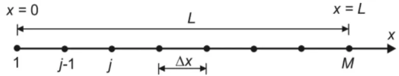
Fig. 1. Solution domain of lengthLcovered by grid points spaced∆x

In the modified FEM approach for the 1D case, where the domain of lengthLwith a structure ofM −1 linear elements is assumed (Fig. 1), the solution of Eq. (3) must

satisfy the following condition:

L Z 0 N(x) ∂Hc ∂t − ∂ ∂x K ∂Ha ∂x !! dx= M−1 X j=1 xj+1 Z xj N(x) ∂Hc ∂t − ∂ ∂x K ∂Ha ∂x !! dx=0, (5) where:

N(x) – vector of linear shape functions, j – index of nodal values,

L – length,

M – number of grid points,

Ha – approximation of the function H(x,t) according to the standard

Galerkin procedure,

Hc – weighted approximation of the function H(x,t) according to the

modified approach.

In the Galerkin procedure, the exact solutionH(x,t) is approximated in the solu-tion domain by the following formula (Fletcher 1991):

H_a(x,t)=N_j(x)·H_j(t)+N_j+1(x)·H_j+1(t), (6) where Hj(t) is the nodal value of the function H(x,t), whereas Nj(x) and Nj+1(x)

represent the linear shape functions which take non-zero values in the elements jand j+1, respectively. The modification of the standard Galerkin procedure is carried out in space dimension during the integration process. According to this approach, the integral of the approximated functionH_aand the shape function can be expressed in each element as follows (Szymkiewicz 2010):

xj+1 Z xj Nj(x)Ha(x,t)dx=Hc(t)∆ x 2 = h ω·Hj(t)+(1−ω)Hj+1(t) i∆x 2 , (7a) xj+1 Z xj Nj+1(x)Ha(x,t)dx=Hc(t)∆ x 2 = h (1−ω)Hj(t)+ωHj+1(t) i∆x 2 , (7b) whereω is a weighting parameter ranging from 0 to 1, and ∆x is the length of an element (distance between nodes). These modified approximations are applied to the time derivative only, whereas the term with the spatial derivative of the 2nd _{order is}

performed by the standard Galerkin approach. In this case, however, because of the application of the linear shape functions, integration by parts for the diffusive term must also be used at first to decrease the order of the derivative. This procedure is carried out for all integrals in Eq. (5). Finally, a global system of ordinary differential equations (ODE) with regard to time is obtained:

• for j =1 ω∆x 2 d H₁ d t +(1−ω) ∆x 2 d H₂ d t − K₁ ∆x(−H1+H2)+K d H d x ₁ =0 , (8a) • for j =2,3, . . . ,M−1

(1−ω)∆x 2 dHj−1 dt +ω·∆x dHj dt +(1−ω) ∆x 2 dHj+1 dt + + Kj−1 ∆x (−Hj−1+Hj) − Kj ∆x(−Hj +Hj+1)=0, (8b) • for j =M (1−ω)∆x 2 dHM−1 dt +ω ∆x 2 dHM dt + KM−1 ∆x (−HM−1+HM) −K dH dx _M =0 , (8c) whereK₁, Kj−1,Kj,KM−1 are the average nodal values of the diffusion coefficient. This system can be rewritten to the matrix form:

AdH

dt +B·H+F=0, (9) where:

H – vector of the nodal values of the unknown functionH(t), A – constant banded matrix of dimensionM×M,

B – variable banded matrix of dimensionM×M, F – vector of the fluxes through the ends.

During the spatial integration of diffusive terms in Eq. (5), it was assumed that the diffusion coefficient is constant over an element and equal to its average valueK. An improper averaging of the diffusion coefficient can cause significant complications during numerical solution. These problems are observed especially for overland flow with a steep wave front or for steady flow over an obstacle. In the latter situation an inaccurate approximation by the standard arithmetic average leads to a unphysical solution, which manifests itself in an excessive accumulation of water volume in the vicinity of the obstacle. One of possible approaches providing satisfactory results for such hydrodynamic conditions is the arithmetic average based on the previously calculated nodal values of the diffusion coefficient (Gąsiorowski 2014):

Kj =

Kj+Kj+1

2 , (10)

where the nodal values of the coefficientsKj andKj+1are given by (see Eq. (4)):

Kj = 1 nh 5/3 j ∂H ∂x −1/2 , (11a) Kj+1= 1 nh 5/3 j+1 ∂H ∂x −1/2 . (11b)

The value of the diffusion coefficient K must be maintained within an appropriate limit in the vicinity of the moving front. For this reason, it is assumed that the diffusion coefficient is equal to zero when the value of water depth is negative or zero, or when the water stage gradient takes a small value, i.e.∂H/∂x< ε, whereε represents the assumed tolerance (Lal 1998). For floodplain application,ε=10−6_{is usually used.}

As far as the time integration of the ODE (9) is concerned, it should be remem-bered that this process corresponds to the solution of an initial value problem. In such a case, the numerical integration of the ODE can be performed by a two-level difference scheme (Szymkiewicz 2010):

Ht+∆t =Ht + ∆t (1−θ) dH dt _t+ θ dH dt _t+∆_t ! , (12)

which, applied for the Eq. (9), leads to the following system of algebraic equations: (A+ ∆t·θ·Bt+∆t)Ht+∆t =(A−∆t(1−θ)Bt)Ht−∆t·θFt+∆t −∆t(1−θ)Ft, (13)

where:

Ht, Ht+∆t – vectors of nodal values at the time levelstandt+ ∆t,

respec-tively,

Bt, Bt+∆t – variable matrixes at the time levelstandt+ ∆t, respectively,

Ft, Ft+∆t – vectors of the fluxes through the ends at the time levelstand

t+ ∆t, respectively,

∆t – time step,

θ – weighting parameter from the range<0,1>.

The resulting system must be closed by boundary conditions imposed at both ends of the domain section considered. Since the Dirichlet condition or an impervious boundary with zero flux will be imposed in the analysis, then the term representing flux by boundary (vectorF) disappears. It is worth adding that the application of the DWE in combination with the FEM makes it possible to find in a natural way the boundaries of the flow that are associated with a moving wet-dry front where the zero depth condition is encountered.

3. Numerical Experiments

In order to estimate the accuracy of the DWE (Eq. (3)) for overland flow, the numer-ical solution of the one-dimensional SWE (Eqs (1)–(2)) is used. Such a solution is treated as a reference solution, which is compared with the one corresponding to the results of calculations obtained by the DWE. For the solution of the SWE, the finite volume method is applied in the form of the wave-propagation algorithm. This algo-rithm, proposed by Leveque (1997), is based on the wave structure of the approximate solution of the Riemann problem. A comprehensive presentation of the algorithm is

given by LeVeque (2002) and Bale et al (2002), and an example of its application in reproducing a dike-break-induced flow has been presented by Gąsiorowski (2011).

3.1. Test 1 – Wave Propagation over a Sloping Bottom

In the numerical test, the one-dimensional wave propagation problem over a dry bot-tom is considered for a rectangular channel of lengthL=4000 m where the Manning roughness coefficientnis equal to 0.05 m−1/3s. Calculations were performed for a bot-tom slope varying in the range of 0≤S≤0.001. Since the initial condition at time

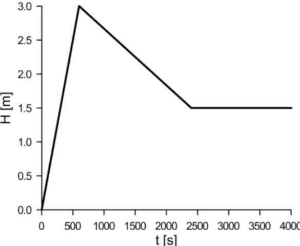
t=0 involves a dry area, then the water levels correspond to the bottom elevations H(x,t=0)=Z(x). However, for the SWE case, a thin film of water over the dry bot-tom must be used to control the small or negative values of water depths that may occur during simulations. For this reason, at the initial time, a constant water depth greater than zero is assumed, i.e.h(x,t=0)=0.01 m. At the upstream boundary end x=0, the inflow boundary condition (Fig. 2) in the form of a water level varying in time is imposed H(x=0,t)=H₀(t). At the downstream end x=L, an impervious boundary with a zero flux∂H/∂x=0 is applied. This boundary is far enough from the domain of solution where a wetting front occurs. In the case of the SWE, an addi-tional initial condition must be imposed. Therefore, zero values are assumed for the depth-averaged velocity at the initial timet =0, i.e.u(x,t =0)=u(x)=0.

Fig. 2. The inflow hydrograph imposed as the upstream boundary condition in Test 1

The computation domain was covered with finite elements ∆x=2 m (Fig. 1). Numerical simulations were run with the time step∆t=2 s for the DWE and with

∆t=0.1 s for the SWE. To avoid unphysical oscillations generated by the algorithm applied, the values of the weighting parameters ω=0.7 in the modified FEM and

θ =0.65 in the two-level difference scheme are used. Such values of the parameters ensure a stable solution, and at the same time numerical diffusion only insignificantly affects the accuracy of the results obtained (Gąsiorowski 2014).

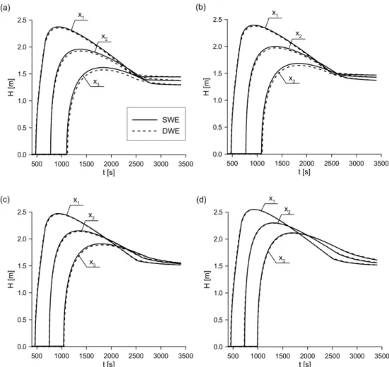
Fig. 3. Computed time series of water levels at selected control points (x₁=500 m,x₂=1000

m,x3=1500 m) for various bottom slopes: (a)S=0; (b)S=0.0001; (c)S=0.0005; (d)S=

0.001

In the first experiment, the effect of the bottom slopeSon the DWE accuracy is examined. A comparison between the SWE and DWE approaches in terms of water level series at selected control points (x₁=500 m, x₂=1000 m, x₃ =1500 m) is given in Fig. 3. Additionally, in each test case, the results of computations are com-pared with respect to the root mean square errorRMS, the relative error in the water level peak EH, and the relative error in time to the position of the wetting frontET.

Theses errors are defined as follows: RMS = s PN t=1 HSW,t−HDW,t2 N , (14) EH = HSW,max−HDW,max HSW,max 100% , (15)

ET = ∆

T

Tmean100%

, (16)

where:

RMS – root mean square error over a period ofNtime steps, HSW,t andHDW,1 – water levels for a given control point computed at

time steptcorresponding to the SWE and DWE, re-spectively,

EH – relative error in the water level peak,

HSW,maxandHDW,max – water level peak corresponding to the SWE and

DWE solutions, respectively,

ET – relative error in time to the position of a wetting

front,

∆T – time difference in terms of the position of wetting fronts between the SWE and DWE solutions, Tmean – average time to the water level peak; in this study

Tmean=600 s is used.

The values ofRMS,EH, andET errors calculated for each variant of the bottom slope

at three selected control points (x₁=500 m,x₂ =1000 m,x₃ =1500 m) are summa-rized in Tab. 1.

Table 1. Impact of bottom slopes onRMS,EH, andET errors computed at selected control

points (x1=500 m,x2=1000 m,x3=1500 m) Slope x₁=500 m x₂=1000 m x₃=1500 m S[-]] RMS EH ET RMS EH ET RMS EH ET [m] [%] [%] [m] [%] [%] [m] [%] [%] 0 0.026 0.83 0.33 0.031 1.61 0.00 0.055 2.69 3.00 0.0001 0.024 0.72 0.67 0.025 1.38 0.33 0.050 2.24 2.67 0.0005 0.021 0.37 0.67 0.018 0.69 0.67 0.033 1.06 1.67 0.001 0.020 0.03 0.67 0.019 0.14 0.67 0.017 0.30 0.67

It can be seen that the results obtained by the DWE approach for a steep slope with S=0.001 (Fig. 3d) are very close to the reference solution, where theRMSerror for the points x₁, x₂, x₃ takes the values between 0.020 and 0.017 m, and the relative errors E_H and E_T are less than 0.7%. However, as the bottom slope decreases, the DWE solution increasingly deviates from the reference solution – for example, at the pointx₃the correspondingRMSerror varies from 0.017 m to 0.055 m. This tendency is especially apparent for small values of slope:S=0.0001 andS=0 (Fig. 3a, Fig. 3b). In these cases, the DWE approach gives a slightly underestimated solution with regard to the peak water level, and the error EH for all control points ranges from

0.72% to 2.69%. The maximal difference between solutions is obtained for a zero bottom slope at the control pointx₃(Fig. 3a), where the correspondingRMS,EH, and

that a similar tendency in the relationship between the bottom slope and the error in the peak water level was reported by Hromadka (1986) for a dam-break-induced flow.

3.2. Test 2 – Wave Propagation over a Hump

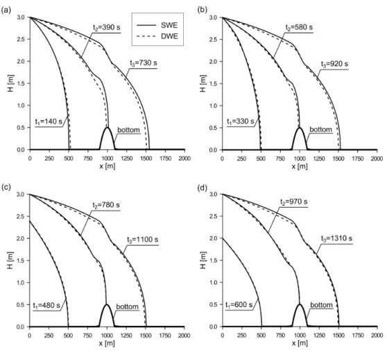
We next consider flood wave propagation over a horizontal bottom with a hump lo-cated in the central part of the domain (Fig. 4a). In this test, the same parameters of channel, spatial discretization, and initial-boundary conditions are used as in the previous test. Only the shape of the inflow hydrograph at the upstream boundary is modified, as it is depicted in Fig. 4b.

Fig. 4. Bathymetry of the domain (a), and the shape of the inflow hydrograph imposed as the

upstream boundary condition in Test 2 (example forT_max=600 s) (b)

Simulations were performed for four variants of the inflow boundary condition, which differ in the timeT_maxto the peak water level. This time ranges from 10 s to 900 s. Such a condition makes it possible to control the rate of flood wave propaga-tion. The imposed hydrograph with a short timeT_maxgenerates a rapidly varied wave, whereas a longer time causes the water wave to propagate freely over the dry area. Figure 5 shows water level profiles computed at selected times, whereas in Fig. 6 the time series at the control pointsx₁ =500,x₂ =1000, andx₃ =1500 m are presented. The results of computations are also compared in terms ofRMS, EH, andET errors,

which are summarized in Tab. 2. These results, in combination with error analysis, indicate that as the rate of wave propagation increases (i.e. timeT_maxdecreases), the solution of the DWE increasingly differs from the reference solution obtained by the SWE. In this case, at the point x₃ theRMS error varies from 0.037 m to 0.091 m, whereas the relative errorETin time to the position of a wetting front ranges from 1%

to 3.67%. For a slowly varied wave withT_max=900 s (Fig. 5d and Fig. 6d), the DWE solution converges with the benchmark solution, where the corresponding errors take low values for all control points (RMS<0.040 m,EH <1.8%, andET ≤1%).

Fig. 5. Computed water level profiles at selected times for various times to the peak water

level at the inflow upstream boundary: (a)Tmax=10 s, (b)Tmax=300 s, (c)Tmax=600 s,

(d)T_max=900 s

differences between the two approaches in the position of fronts occur at the pointx₂ which is located on a hump. For the shortest timeT_max=10 s (Fig. 5a), theRMSand ET errors calculated at the point x2take the maximal values of 0.073 m and 2.33%,

respectively. In this case, flow in the vicinity of the hump has a more complex structure than at other points of the computational domain. Consequently, the simplified diffu-sive wave model cannot accurately reproduce such local hydrodynamic phenomena because of the lack of an inertial term. It is worth noting that the imposed condition with a short time to the peak water level (T_max=10 s) generates a rather rapid wave in comparison with those that can be observed in floodplain inundation problems. In a typical dike-break-induced flow, the wave propagates more gradually over a few minutes rather than seconds. Therefore, it seems that the algorithm applied is capable of reproducing the flood wave propagation over a dry floodplain with good accuracy.

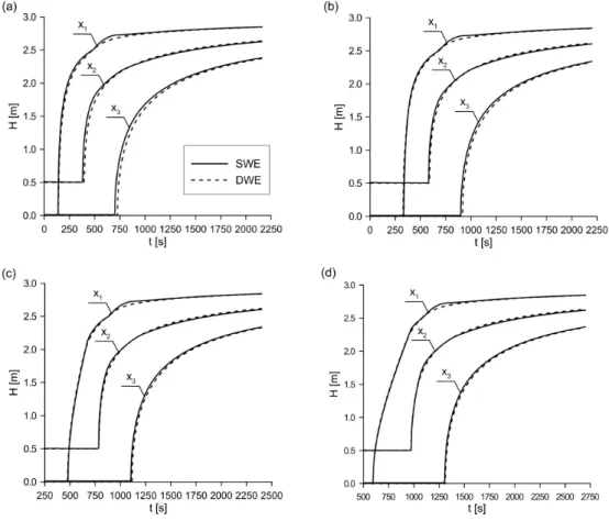
Fig. 6. Computed time series of water levels at selected control points (x1=500 m,x2=1000

m,x3=1500 m) for various times to the peak water level at the inflow upstream boundary: (a) T_max=10 s, (b)T_max=300 s, (c)T_max=600 s, (d)T_max=900 s

Table 2. Impact of time to the peak water level onRMS,EH, andET errors computed at

selected control points (x1=500 m,x2=1000 m,x3=1500 m) T_max x₁=500 m x₂=1000 m x₃=1500 m [s] RMS EH ET RMS EH ET RMS EH ET [m] [%] [%] [m] [%] [%] [m] [%] [%] 10 0.043 1.88 1.00 0.073 −0.58 2.33 0.091 1.11 3.67 300 0.040 1.75 0.67 0.047 −0.74 1.00 0.068 0.98 2.00 600 0.027 1.69 0.33 0.026 −0.81 0.33 0.055 0.82 1.67 900 0.020 1.72 0.00 0.020 −0.88 0.33 0.037 0.70 1.00 4. Conclusions

In this paper, the numerical solution of the one-dimensional DWE was compared with the corresponding reference solution of the SWE obtained by means of the finite

volume methods. The accuracy of the DWE was evaluated by two numerical experi-ments, in which the propagation of a flood wave over a dry bottom was simulated. The tests were carried out for various bottom slopes, as well as for different shapes of the upstream boundary conditions. The results obtained indicate that, although the sim-plified diffusive model does not include the inertia force, it can effectively reproduce floodplain inundation. The numerical algorithm applied to the solution of the DWE gives accurate results for slowly varied waves, as well as for steep bottom slopes. In the case of a rapidly varied wave over a hump, the diffusive wave approximation gives a slightly inaccurate solution. In spite of that, it seems that the DWE approach can be employed in combination with the FEM for the modeling of wave propagation prob-lems where we need to determine the boundaries of a floodplain temporarily covered by water. It should be emphasized, however, that the preliminary results obtained for one-dimensional flow cannot be directly extended to a two-dimensional problem. This aspect of modeling needs further investigation.

References

Abbot M. B. (1979)Computational hydraulics – elements of the theory of free surface flow, Pitman.

Bale D. S., LeVeque R. J., Mitran S., Rossmanith J. A. (2002) A wave propagation method for conser-vation laws and balance laws with spatially varying flux functions,SIAM, J. Sci. Comput.,24(3),

995–978.

Bates P. D., Horrit M. S., Fewtrell T. J. (2010) A simple inertial formulation of the shallow water equa-tions for efficient two-dimensional flood inundation modelling,Journal of Hydrology,387, 33–45.

Begnudelli L., Sanders B. F. (2006) Unstructured grid finite-volume algorithm for shallow-water flow and scalar transport with wetting and drying, Journal of Hydraulic Engineering, 132 (4), 371–384. Cunge J. A. (1975) Two-dimensional modeling of flood plains. [In]: K. Mahmood, and V. Yevjevich (eds.),Unsteady flow in open channels, vol. II, Water Resources Publications, Collins, Colorado,

USA, 705–762.

Fletcher C. A. J. (1991)Computational techniques for fluid dynamics, vol. I, Springer-Verlag.

Gąsiorowski D.(2011) Solution of the dike-break problem using finite volume method and splitting technique,TASK Quarterly,15(3–4), 251–270.

Gąsiorowski D. (2013) Analysis of floodplain inundation using 2D nonlinear diffusive wave equation solved with splitting technique,Acta Geophysica,61(3), 668–689.

Gąsiorowski D. (2014) Impact of diffusion coefficient averaging on solution accuracy of the 2D nonlin-ear diffusive wave equation for floodplain inundation,Journal of Hydrology,517, 923–935.

Gourgue O., Comblen R., Lambrechts J., Kärnä T., Legat V., Deleersnijder (2009) A flux-limiting wetting–drying method for finite-element shallow-water models, with application to the Scheldt Estuary,Advances in Water Resources,32, 1726–1739.

Heniche M., Secretan Y., Boudreau P., Leclerc M. (2000) A two-dimensional finite drying-wetting shal-low water model for rivers and estuaries,Advances in Water Resources,23, 359–372.

Horritt M. S. (2002) Evaluating wetting and drying algorithms for finite element models of shallow water flow,International Journal for Numerical Methods in Engineering,55, 835–851.

Horrit M. S., Bates P. D. (2002) Evaluation of 1D and 2D numerical models for predicting river flood inundation,Journal of Hydrology,268, 87–99.

Hromadka T. V. (1985) Predicting Dam-Break Flood Depths Using A One-Dimensional Diffusion Model,Microsoftware For Engineers,1(1), 22–31.

Hromadka T. V., Yen C. C. (1986) A diffusion hydrodynamic model (DHM),Advances in Water Re-sources,9, 118–170.

Hsu M. H., Chen S. H., Chang T. J. (2000) Inundation simulation for urban drainage basin with storm sewer system,Journal of Hydrology,234, 21–37.

Lal A. M. W. (1998) Performance comparison of overland flow algorithms,Journal of Hydraulic Engi-neering,124(4), 342–349.

LeVeque R. J. (2002)Finite volume methods for hyperbolic problems, Cambrige University Press.

LeVeque R. J. (1997) Wave Propagation Algorithms for Multidimensional Hyperbolic Systems,Journal of Computational Physics,131, 327–353.

Liang Q., Borthwick A. G. L. (2009) Adaptive quadtree simulation of shallow flow with wet-dry fronts over complex topography,Computers and Fluids,38, 221–234.

Moussa R., Bocquillon C. (2009) On the use of the diffusive wave for modeling extreme flood events with overbank flow in the floodplain,Journal of Hydrology,374, 116–135.

Neal J., Villanueva I., Wright N., Willis T., Fewtrell T., Bates P. (2011) How much physical complexity is needed to model flood inundation?,Hydrological Processes,26(15), 2264–2282.

Oritz P. (2013) Shallow water flows over flooding areas by a flux-corrected finite element method,

Journal of Hydraulic Research,52, 2, 241–252,

Prestininzi P. (2008) Suitability of the diffusive model for dam break simulation application to a CADAM experiment,Journal of Hydrology,361, 172–185.

Singh V. P. (1996)Kinematic wave modeling in water resources, John Wiley & Sons, Inc. New York.

Szydłowski M. (2007) Mathematical modeling of flood waves in urban areas, Monographs of Gdańsk University of Technology , vol. 86, Gdańsk (in Polish).

Szydłowski M. (2008) Two-dimensional diffusion wave model for numerical simulation of inundation – Narew case study,Publs. Inst. Geophys. Pol. Acad. Sc., E-9, 405, 107–120.

Szydłowski M., Magnuszewski A. (2007) Free surface flow modeling in numerical estimation of flood risk zones: a case study, Gdańsk, TASK Quarterly, 11 (4), 301–313.

Szymkiewicz R. (1995) Method to solve 1D unsteady transport and flow equations,Journal of Hydraulic Engineering ASCE,121(5), 396–403.

Szymkiewicz R. (2010)Numerical modeling in open channel hydraulics, Water Science and Technology

Library, Springer, New York.

Szymkiewicz R., Gąsiorowski D. (2012) Simulation of unsteady flow over floodplain using the diffusive wave equation and the modified finite element,Journal of Hydrology,464–465, 165–167.

Tan W. (1992)Shallow water hydrodynamics, Elsevier, Amsterdam.

Zhang X. H., Ishidaira H., Takeuchi K., Xu Z. X., Zhuang X. W. (2004) An approach to inundation in large river basins using the triangle finite difference method,Journal of Environmental Informatics,