Rose Yu* 1 Stephan Zheng* 1 Anima Anandkumar1 Yisong Yue1
Abstract
We present Tensor-Train RNN (TT-RNN), a novel family of neural sequence architectures for multi-variate forecasting in environments with nonlinear dynamics. Long-term forecasting in such systems is highly challenging, since there exist long-term temporal dependencies, higher-order correlations and sensitivity to error propagation. Our proposed tensor recurrent architecture addresses these is-sues by learning the nonlinear dynamics directly using higher order moments and high-order state transition functions. Furthermore, we decompose the higher-order structure using the tensor-train (TT) decomposition to reduce the number of pa-rameters while preserving the model performance. We theoretically establish the approximation prop-erties of Tensor-Train RNNs for general sequence inputs, and such guarantees are not available for usual RNNs. We also demonstrate significant long-term prediction improvements over general RNN and LSTM architectures on a range of sim-ulated environments with nonlinear dynamics, as well on real-world climate and traffic data.
1. Introduction
One of the central questions in science is forecasting: given the past history, how well can we predict the future? In many domains with complex multi-variate correlation structures and nonlinear dynamics, forecasting is highly challenging since the system has long-term temporal dependencies and higher-order dynamics. Examples of such systems abound in science and engineering, from biological neural network activity, fluid turbulence, to climate and traffic systems (see Figure1). Since current forecasting systems are unable to faithfully represent the higher-order dynamics, they have limited ability for accuratelong-termforecasting.
Therefore, a key challenge is accurately modeling nonlinear
*
Equal contribution 1Department of Computing and Math-ematical Sciences, Caltech, Pasadena, USA. Correspon-dence to: Rose Yu <[email protected]>, Stephan Zheng <[email protected]>.
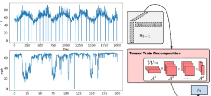
Figure 1.Left: climate and traffic time series per location. The time-series exhibits long-term temporal correlations, and can be viewed as a realization of highly nonlinear dynamics. Right: tensor-train RNN unit encodes high-order dynamics and factorizes hidden states with tensor train decomposition.
dynamics and obtaining stable long-term predictions, given a dataset of realizations of the dynamics. Here, the forecast-ing problem can be stated as follows: how can we efficiently learn a model that, given only few initial states, can reliably predict a sequence of future states over a long horizon ofT
time-steps?
Common approaches to forecasting involve linear time series models such as auto-regressive moving average (ARMA), state space models such as hidden Markov model (HMM), and deep neural networks. We refer readers to a sur-vey on time series forecasting by (Box et al.,2015) and the references therein. A recurrent neural network (RNN), as well as its memory-based extensions such as the LSTM, is a class of models that have achieved good performance on se-quence prediction tasks from demand forecasting (Flunkert et al.,2017) to speech recognition (Soltau et al.,2016) and video analysis (LeCun et al.,2015). Although these meth-ods can be effective for short-term, smooth dynamics, they can hardly generalize to nonlinear dynamics and make pre-dictions over longer time horizons.
To address this issue, we propose a novel family of tensor-train recurrent neural networks that can learn stable long-term forecasting. These models have two key features: they 1)explicitly model the higher-order dynamics, by using a longer history of previous hidden states and high-order state interactions with multiplicative memory units; and 2) they are scalable by usingtensor trains, a structured low-rank tensor decomposition that greatly reduces the number of model parameters, while mostly preserving the correlation
structure of the full-rank model.
In this work, we analyze Tensor-Train RNNs theoretically, and also validate them experimentally over a wide range of forecasting domains. Our contributions can be summarized as follows:
• We describe howTT-RNNs encode higher-order non-Markovian dynamics and high-order state interactions. To address the memory issue, we propose a tensor-train (TT) decomposition that makes learning tractable and fast.
• We provide theoretical guarantees for the representa-tion power ofTT-RNNs for nonlinear dynamics, and obtain the connection between the target dynamics and TT-RNNapproximation. In contrast, no such theoreti-cal results are known for standard recurrent networks. • We validateTT-RNNs on simulated data and two real-world environments with nonlinear dynamics (climate and traffic). Here, we show thatTT-RNNs can forecast more accurately for significantly longer time horizons compared to standard RNNs and LSTMs.
2. Related Work
Classic work in time series forecasting has studied auto-regressive models, such as the ARMA or ARIMA model (Box et al., 2015), which model a processx(t) linearly, and so do not capture nonlinear dynamics. Using neural networks to model time series data has a long history. Neu-ral sequence models have been applied to room tempera-ture prediction, weather forecasting, traffic prediction and many other domains. We refer to (Schmidhuber,2015) for a detailed overview of the relevant literature. Recent devel-opment in deep leaning and RNNs has led to forecasting models such as deep AutoRegressive (Flunkert et al.,2017) and Predictive State Representation (Downey et al.,2017). However, RNNs only use the most recent hidden state and can be restrictive in modeling higher-order dynamics. Our method contrasts with this by explicitly modeling higher-order dependencies.
From a modeling perspective, (Giles et al.,1989) considers ahigh-order RNNto simulate a deterministic finite state ma-chine and recognize regular grammars. This work considers a second order mapping from inputsx(t)and hidden states
h(t)to the next state. However, this model only considers the most recent state and is limited to two-way interactions. (Sutskever et al.,2011) proposesmultiplicative RNNthat allow each hidden state to specify a different factorized hidden-to-hidden weight matrix. A similar approach also appears in (Soltani & Jiang,2016), but without the factor-ization. Moreover, hierarchical RNNs have been used to model sequential data at multiple resolutions, e.g. to learn
both short-term and long-term human behavior (Zheng et al., 2016). Our method can be seen as an efficient generalization of these works where we model the high-order interactions using a hidden-to-hidden tensor.
Tensor methods have tight connections with neural networks. For example, (Novikov et al.,2015;Stoudenmire & Schwab, 2016) employs tensor-train as model compression tool to reduce the number of weights in neural networks. (Yang et al.,2017) further extends this idea to RNNs by reshap-ing the inputs into a tensor and factorizes the input-hidden weight tensor. However, the purpose of these works is model compression whereasTT-RNNaims to learn a high-order states transition function. Theoretically, (Cohen et al.,2016) shows convolutional neural networks are equivalent to hier-archical tensor factorizations. Mostly recently, (Khrulkov et al.,2017) provides expressiveness analysis for shallow network with tensor train models. This work however, to the best of our knowledge, is the first work to consider ten-sor networks in RNNs for sequential prediction tasks for learning in environments with nonlinear dynamics.
3. Forecasting using Tensor-Train RNNs
Forecasting Nonlinear Dynamics Our goal is to learn an efficient modelfforsequential multivariate forecastingin environments with nonlinear dynamics. Such systems are governed bydynamicsthat describe how a system statext∈ Rdevolves using a set ofnonlineardifferential equations:ξi xt, dx dt, d2x dt2, . . .;φ = 0 i , (1)
whereξican be an arbitrary (smooth) function of the state
xtand its derivatives. Continous time dynamics are usually described by differential equations while difference equa-tions are employed for discrete time. In continuous time, a classic example is the first-order Lorenz attractor, whose realizations showcase the “butterfly-effect”, a characteristic set of double-spiral orbits. In discrete-time, a non-trivial example is the 1-dimensional Genz dynamics, whose differ-ence equation is:
xt+1= c−2+ (xt+w)2
−1
, c, w∈[0,1], (2) wherextdenotes the system state at timetandc, ware the parameters. Due to the nonlinear nature of the dynamics, such systems exhibit higher-order correlations, long-term dependencies and sensitivity to error propagation, and thus form a challenging setting for learning.
Given a sequence of initial statesx0. . .xt, the forecasting
problem aims to learn a modelf
that outputs a sequence of future statesxt+1. . .xT. Hence, accurately approximating the dynamicsξis critical to learn-ing a good forecastlearn-ing modelf and accurately predicting for long time horizons.
First-order Markov Models In deep learning, common approaches for modeling dynamics usually employ first-order hidden-state models, such as recurrent neural networks (RNNs). An RNN with a single cell recursively computes a hidden statehtusing the most recent hidden stateht−1,
generating the outputytfrom the hidden stateht:
ht=f(xt,ht−1;θ), yt=g(ht;θ), (4) where f is the state transition function, g is the output function and θ are the model parameters. A common parametrization scheme for (4) is a nonlinear activation function applied to a linear map ofxtandht−1as:
ht=f(Whxxt+Whhht−1+bh), (5)
xt+1=Wxhht+bx, (6) where the state transitionf can be sigmoid, tanh, etc.,
Whx, Wxh andWhh are transition weight matrices and
bh,bxare biases.
RNNs have many different variations, including LSTMs (Hochreiter & Schmidhuber,1997) and GRUs (Chung et al., 2014). For instance, LSTM cells use a memory-state, which mitigate the “exploding gradient” problem and allow RNNs to propagate information over longer time horizons. Al-though RNNs are very expressive, they compute the hidden statehtusing only the previous stateht−1 and input xt.
Such models do not explicitly model higher-order dynamics and only capture long-term dependencies between all histor-ical statesh0. . .htimplicitly, which limits their forecasting effectiveness in environments with nonlinear dynamics. 3.1. Tensorized Recurrent Neural Networks
To effectively learn nonlinear dynamics, we propose Tensor-Train RNNs, orTT-RNNs, a class of higher-order models that can be viewed as a higher-order generalization of RNNs. We developedTT-RNNs with two goals in mind: explicitly modeling 1) L-order Markov processes with L steps of temporal memory and 2) polynomial interactions between the hidden statesh·andxt.
First, we consider longer “history”: we keep lengthL his-toric states:ht,· · ·,ht−L:
ht=f(xt,ht−1,· · ·,ht−L;θ) (7) wherefis an activation function. In principle, early work (Giles et al., 1989) has shown that with a large enough hidden state size, such recurrent structures are capable of approximating any dynamics.
Second, to learn the nonlinear dynamicsξefficiently, we also use higher-order moments to approximate the state transition function. Concatenate theL-lag hidden state as an augmented statest−1:
sTt−1= [1 h>t−1 . . . h>t−L]
For every hidden dimension, we construct aP-dimensional transitionweight tensorby modeling a degreePpolynomial interaction between hidden states:
[ht]α=f(Wαhxxt+ (8) X i1,···,ip Wαi1···iPst−1;i1⊗ · · · ⊗st−1;ip | {z } P )
whereαindices the hidden dimension,i·indices the
high-order terms andP is the polynomial order. We included the bias unit1inst−1to account for the first order term, so that
st−1;i1⊗ · · · ⊗st−1;ipcan model all possible polynomial
expansions up to orderP.
TheTT-RNNwith LSTM cell, or “TLSTM”, is defined analogously as: [it,gt,ft,ot]α=σ(Wαhxxt+ X i1,···,ip Wαi1···iPst−1;i1⊗ · · · ⊗st−1;iP | {z } P ), (9) ct=ct−1◦ft+it◦gt, ht=ct◦ot where◦denotes the Hadamard product. Note that the bias units are again included.
TT-RNNis a basic unit that can be incorporated in most of the existing recurrent neural architectures such as con-volutional RNN (Xingjian et al.,2015) and hierarchical RNN (Chung et al.,2016). In this work, we useTT-RNN as a module for sequence-to-sequence (Seq2Seq) frame-work (Sutskever et al.,2014) in order to perform long-term forecasting.
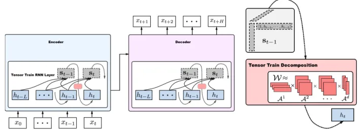
As shown in Figure2, sequence-to-sequence consists of an encoder-decoder pair. Encoder takes an input sequence and learns a hidden representation. Decoder initializes with this hidden representation and generates an output sequence. Both contains multiple layers of tensor-train recurrent cells (color coded in red). The augmented statest−1(color coded
in grey) concatenates the past Lhidden states. And the tensor-train cell takesst−1and outputs the next hidden state.
The encoder encodes the initial statesx0, . . . , xt and the decoder predictsxt+1, . . . , xT. For each timestept, the decoder uses its own previous predictionytas an input. 3.2. Tensor-train Networks
Unfortunately, due to the “curse of dimensionality”, the number of parameters inWαwith hidden sizeHgrows ex-ponentially asO(HLP), which makes the high-order model
Figure 2.Tensor-train recurrent cells within a seq2seq model. Both encoder and decoder contain tensor-train recurrent cells. The augmented statest−1(grey) takes in pastLhidden states (blue) and forms a high-order tensor. Tensor-train cell (red) factorizes the tensor and outputs the next hidden state.
Figure 3.A tensor-train cell. The aug-mented state st−1 (grey) forms a high-order tensor, which is then factorized to output the next hidden state.
prohibitively large to train. To overcome this difficulty, we utilizetensor networksto approximate the weight tensor. Such networks encode a structural decomposition of tensors into low-dimensional components and have been shown to provide the most general approximation to smooth tensors (Or´us,2014). The most commonly used tensor networks are linear tensor networks(LTN), also known astensor-trains in numerical analysis ormatrix-product statesin quantum physics (Oseledets,2011).
A tensor train model decomposes aP-dimensional tensor Winto a network of sparsely connected low-dimensional tensors{Ap∈ Rrp−1×np×rp}as: Wi1···iP = X α1···αP−1 A1α0i1α1A 2 α1i2α2· · · A P αP−1iPαP
with α0 = αP = 1, as depicted in Figure (3). When
r0=rP = 1the{rp}are called the tensor-train rank. With tensor-train, we can reduce the number of parameters of TT-RNNfrom(HL+ 1)P to(HL+ 1)R2P, withR =
maxprpas the upper bound on the tensor-train rank. Thus, a major benefit of tensor-train is that theydo notsuffer from the curse of dimensionality, which is in sharp contrast to many classical tensor decomposition models, such as the Tucker decomposition.
4. Approximation results for TT-RNN
A significant benefit of using tensor-trains is that we can theoretically characterize the representation power of tensor-train neural networks for approximating high-dimensional functions. We do so by analyzing a class of functions that satisfies certain regularity conditions.
In the context of TT-RNN, the target function f(x)
de-scribes the underlying system dynamics, as in (9). We first show that iff preserves weak derivatives, it has a compact tensor train representation. Formally, let us assume thatf
is a Sobolev function:f ∈ Hk
µ, defined on the input space I = I1×I2× · · ·Id, where each Ii is a set of vectors. The spaceHk
µis defined as the functions that have bounded derivatives up to some orderkand areLµ-integrable:
Hkµ= f ∈Lµ(I) : X i≤k kD(i)fk2<+∞ , (10)
whereD(i)f is thei-th weak derivative off andµ≥0.1 It is known that any Sobolev function admits a Schmidt decomposition:f(·) =P∞
i=0
p
λ(i)γ(·;i)⊗φ(i;·), where {λ} are the eigenvalues and {γ},{φ}are the associated eigenfunctions. Hence, we can represent the state transition functionf(x)as an infinite summation of products of a set of basis functions: f(x) = ∞ X α0,···,αd=1 A1(α 0, x1, α1)· · · Ad(αd−1, xd, αd), (11) where{Ad(α d−1, sd, αd) = p λd−1(αd−1)φ(αd−1;sd)} are basis functions over each input dimension. Such basis function satisfieshAd(i,·, m),Ad(i,·, m)i=δmn. Functional tensor-train(FTT) truncates (17) to a low dimen-sional subspace (r<∞), and obtain a functional
approxi-1A weak derivative generalizes the derivative concept for
(non)-differentiable functions and is implicitly defined as: e.g. v ∈
L1([a, b])is a weak derivative ofu∈L1([a, b])if for all smooth ϕwithϕ(a) =ϕ(b) = 0:Rb
au(t)ϕ
0
(t) =−Rb
mation of the state transition functionf(x): fF T T(x) = r X α0,···,αd A1(α 0, x1, α1)· · · Ad(αd−1, xd, αd), (12)
In practice,TT-RNNimplements a polynomial expansion of the states using[s,s⊗2,· · · ,s⊗P], wherePis the degree of the polynomial. The final function that is represented by TT-RNNis a polynomial approximation of the functional tensor-train functionfF T T.
Given a target functionf, and a neural network with one hidden layer and sigmoid activation function, the following lemma describes the classic result of describing the error betweenf and the single hidden-layer neural network that approximates it best:
Lemma 4.1(NN Approximation (Barron,1993)). Given a functionfwith finite Fourier magnitude distributionCf, there exists a neural network ofnhidden unitsfn, such that
kf−fnk ≤ Cf √ n (13) whereCf = R
|ω|1|fˆ(ω)|dωwith Fourier representation
f(x) =R eiωxfˆ(ω)dω.
We can generalize Barron’s approximation result in lemma .3toTT-RNN. The target function we are approximating with neural networks is the state transition functionf(x) = f(s⊗ · · · ⊗s). We can express this function using FTT, followed by the polynomial expansion of the states. The following theorem characterizes the representation power ofTT-RNN, viewed as a one-layer hidden neural network, in terms of 1) the regularity of the target function
f, 2) the dimension of the input space, 3) the tensor train rank and 4) the order of the tensor:
Theorem 4.2. Let the state transition functionf ∈ Hk µbe a H¨older continuous function defined on a input domain I =I1× · · · ×Id, with bounded derivatives up to order
k and finite Fourier magnitude distribution Cf. Then a single layer Tensor Train RNN can approximatefwith an estimation error ofusing withhhidden units:
h≤ C 2 f (d−1) (r+ 1)−(k−1) (k−1) + C2 f C(k)p −k (14)
whereCf=R |ω|1|fˆ(ω)dω|,dis the size of the state space,
ris the tensor-train rank andpis the degree of high-order polynomials i.e., the order of tensor.
For the full proof, see the Appendix.
From this theorem we see: 1) if the targetf is simple with low-dimensional states (smalld), it is easier to approximate
and 2) polynomial interactions are more efficient than lin-ear ones in the large rank region: if the polynomial order increases (largep), we require fewer hidden unitsh. This re-sult applies to the full family ofTT-RNNs, including those using vanilla RNN or LSTM as the recurrent cell, as long as we are given a state transitions(xt,st)7→st+1(e.g. the
state transition function learned by the encoder).
5. Experiments
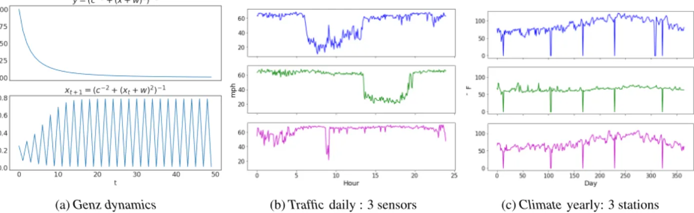
We validated the accuracy and efficiency ofTT-RNNon one synthetic and two real-world datasets, as described below; We performed missing data imputation and used rolling window to extract input-output subsequences. Detailed pre-processing and data statistics are deferred to the Appendix. Genz dynamics The Genz “product peak” (see Figure4 a) is one of the Genz functions (Genz,1984), which are often used as a basis for high-dimensional function approximation. In particular, (Bigoni et al., 2016) used them to analyze tensor-train decompositions. We generated10,000samples time series of length100using (2) withw= 0.5, c= 1.0
and random initial points.
Traffic The traffic data (see Figure4 b) of Los Angeles County highway network is collected from California depart-ment of transportation http://pems.dot.ca.gov/. The prediction task is to predict the speed readings for15
locations across LA, aggregated every5minutes. After up-sampling and processing the data for missing values, we obtained8,784sequences of length288.
Climate The climate data (see Figure 4 c) is col-lected from the U.S. Historical Climatology Net-work (USHCN) (http://cdiac.ornl.gov/ftp/ ushcn_daily/). The prediction task is to predict the daily maximum temperature for15stations. The data spans approximately124years. After preprocessing, we obtained
6,954sequences of length366.
5.1. Long-term Forecasting Evaluation
Experimental Setup To validate that TT-RNNs effec-tively perform long-term forecasting task in (3), we ex-periment with a seq2seq architecture withTT-RNNusing LSTM as recurrent cells (TLSTM). For all experiments, we used an initial sequence of lengtht0as input and varied the
forecasting horizonT. We trained all models using stochas-tic gradient descent on the length-T sequence regression lossL(y,y) =ˆ PTt=1||yˆt−yt||22,whereyt=xt+1,yˆtare the ground truth and model prediction respectively. We comparedTT-RNNagainst 2 set of natural baselines: 1st-order RNN (vanilla RNN, LSTM), and matrix RNNs (vanilla MRNN, MLSTM), which use matrix products of
(a)Genz dynamics (b)Trafficdaily : 3 sensors (c)Climateyearly: 3 stations Figure 4.Data visualizations: (4a) Genz dynamics, (4b) traffic data, (4c) climate data.
(a)Genz dynamics (b)Traffic (c)Climate
Figure 5.Long-term forecasting RMSE forGenz dynamicsand real worldtraffic,climatetime series (best viewed in color). Comparison of LSTM, MLSTM, and TLSTM for varying forecasting horizons given same initial inputs. Results are averaged over3runs.
multiple hidden states without factorization (Soltani & Jiang, 2016). We observed thatTT-RNNwith RNN cells outforms vanilla RNN and MRNN, but using LSTM cells per-forms best in all experiments. We also evaluated the classic ARIMA time series model with AR lags of1∼5, and MA lags of1 ∼ 3. We observed that it consistently performs ∼5%worse than LSTM.
Training and Hyperparameter Search We trained all models using the RMS-prop optimizer and employed a learn-ing rate decay of0.8schedule. We performed an exhaustive search over the hyper-parameters for validation. Table3 reports the hyper-parameter search range used in this work. For all datasets, we used a 80% −10% −10% train-validation-test split and train for a maximum of1e4steps. We compute the moving average of the validation loss and use it as an early stopping criteria. We did not employ sched-uled sampling (Bengio et al.,2015), as we found training became unstable under a range of annealing schedules. The number of parameters of best performing models are listed in Table3. The TLSTM model is comparable with that of MLSTM and LSTM. More parameters would cause overfitting. TLSTM is more flexible than other methods,
Table 1.Hyper-parameter search range statistics forTT-RNN ex-periments and the best performing model size for all models.
Hyper-parameter Range
LEARNING RATE TENSOR RANK HIDDEN SIZE
10−1 ∼10−5 1∼16 8∼128
#OF LAGS #OF ORDERS #OF LAYERS
1∼6 1∼3 1∼3
Best Performing Model Size
TLSTM MLSTM LSTM
7.2K 9.7K 8.7K
which gives us better control of the model complexity. Long-term Accuracy Fortraffic, we forecast up to 18
hours ahead with 5 hours as initial inputs. Forclimate, we forecast up to300days ahead given60days of initial observations. ForGenz dynamics, we forecast for80steps given5initial steps. All results are averages over3runs. We now present the long-term forecasting accuracy of TL-STM in nonlinear systems. Figure5shows the test predic-tion error (in RMSE) for varying forecasting horizons for
Figure 6.Model prediction for three realizations with different intiial conditions for Genz dynamics “product peak”. Top (blue): ground truth. Bottom: model predictions for LSTM (green) and TLSTM (red). TLSTM perfectly captures the Genz oscillations, whereas the LSTM fails to do so (left) or only approaches the ground truth towards the end (middle and right).
Figure 7.Top:18hour ahead predictions for hourlytraffictime series given5hour as input for LSTM, MLSTM and TLSTM. Bottom:
300days ahead predictions for dailyclimatetime series given2month observations as input for LSTM, MLSTM and TLSTM. different datasets. We can see that TLSTM notably
outper-forms all baselines on all datasets in this setting. In particu-lar, TLSTM is more robust to long-term error propagation. We observe two salient benefits of using TT-RNNs over the unfactorized models. First, MRNN and MLSTM can suffer from overfitting as the number of weights increases. Second, ontraffic, unfactorized models also show consider-able instability in their long-term predictions. These results suggest that tensor-train neural networks learn more stable representations that generalize better for long-term horizons. Visualization of Predictions To get intuition for the learned models, we visualize the best performing TLSTM and baselines in Figure6for the Genz function “corner-peak” and the state-transition function. We can see that TLSTM can almost perfectly recover the original function,
while LSTM and MLSTM only correctly predict the mean. These baselines cannot capture the dynamics fully, often predicting an incorrect range and phase for the dynamics. In Figure7we show predictions for the real world traffic and climate dataset. This work uses deterministic models, hence the predictions correspond to the trend. We can see that the TLSTM aligns significantly better with ground truth in long-term forecasting. As the ground truth time series is highly nonlinear and noisy, LSTM often deviates from the general trend. While both MLSTM and TLSTM can correctly learn the trend, TLSTM captures more detailed curvatures due to the inherent high-order structure.
Speed Performance Trade-off We now investigate po-tential trade-offs between accuracy and computation. Figure
TLSTM Prediction Error (RMSE×10−2 ) TENSOR RANKr 2 4 8 16 GENZ(T= 95) 0.82 0.93 1.01 1.01 TRAFFIC(T= 67) 9.17 9.11 9.32 9.31 CLIMATE(T = 360) 10.55 10.25 10.51 10.63
TLSTM Traffic Prediction Error (RMSE×10−2)
NUMBER OF LAGSL 2 4 5 6
T = 12 7.38 7.41 7.43 7.41 T = 84 8.97 9.31 9.38 9.01
T = 156 9.49 9.32 9.48 9.31
T = 228 10.19 9.63 9.58 9.94 Table 2.TLSTM performance for various tensor-train hyperparameters. Top: varying tensor rankrwithL= 3. Bottom: varying number of lagsLand prediction horizonT.
Figure 8.Training speed evaluation of different models: valida-tion loss versus number of steps. Results are reported using the models with the best long-term forecasting accuracy.
(a) Lorenz Attractor (b)T = 20 (c)T = 40 (d)T = 60 (e)T = 80 6
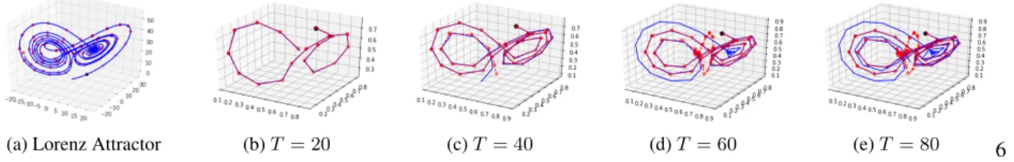
Figure 9.9aLorenz attraction with dynamics (blue) and sampled data (red).9b,9c,9d,9eTLSTM long-term predictions for different forecasting horizonsTversus the ground truth (blue). TLSTM shows consistent predictions over increasing horizonsT.
8displays the validation loss with respect to the number of steps, for the best performing models on long-term fore-casting. We see thatTT-RNNs converge faster than other models, and achieve lower validation-loss. This suggests thatTT-RNNhas a more efficient representation of the non-linear dynamics, and can learn much faster as a result. Hyper-parameter Analysis The TLSTM model is equipped with a set of hyper-parameters, such as tensor-train rank and the number of lags. We perform a random grid search over these hyper-parameters and showcase the results in Table2. In the top row, we report the prediction RMSE for the largest forecasting horizon w.r.t tensor ranks for all the datasets with lag3. When the rank is too low, the model does not have enough capacity to capture non-linear dynamics. when the rank is too high, the model starts to overfit. In the bottom row, we report the effect of changing lags (degree of orders in Markovian dynamics). For each setting, the bestris determined by cross-validation. For different forecasting horizon, the best lag value also varies. Chaotic Nonlinear Dynamics We have also evaluated TT-RNNon long-term forecasting forchaoticdynamics, such as the Lorenz dynamics (see Figure99a). Such dy-namics are highly sensitive to input perturbations: two close points can move exponentially far apart under the dynamics.
This makes long-term forecasting highly challenging, as small errors can lead to catastrophic long-term errors. Fig-ure9shows thatTT-RNNcan predict up toT = 40steps into the future, but diverges quickly beyond that. We have found no state-of-the-art prediction model is stable beyong
40time stamps in this setting.
6. Conclusion and Discussion
In this work, we considered long-term forecasting under nonlinear dynamics. We propose a novel class of RNNs – TT-RNNthat directly learns the nonlinear dynamics. We provide the first approximation guarantees for it represen-tation power. We demonstrate the benefits ofTT-RNNto forecast accurately for significantly longer time horizon in both synthetic and real-world multivariate time series data. As we observed, chaotic dynamics still present a significant challenge to any sequential prediction model. Hence, it would be interesting to study how to learn robust models for chaotic dynamics. In other sequential prediction settings, such as natural language processing, there does not (or is not known to) exist a succinct analytical description of the data-generating process. It would be interesting to go be-yond forecasting and further investigate the effectiveness of TT-RNNs in such domains as well.
References
Barron, Andrew R. Universal approximation bounds for su-perpositions of a sigmoidal function. IEEE Transactions on Information theory, 39(3):930–945, 1993.
Bengio, Samy, Vinyals, Oriol, Jaitly, Navdeep, and Shazeer, Noam. Scheduled sampling for sequence prediction with recurrent neural networks. InAdvances in Neural Infor-mation Processing Systems, pp. 1171–1179, 2015. Bigoni, Daniele, Engsig-Karup, Allan P, and Marzouk,
Youssef M. Spectral tensor-train decomposition. SIAM Journal on Scientific Computing, 38(4):A2405–A2439, 2016.
Box, George EP, Jenkins, Gwilym M, Reinsel, Gregory C, and Ljung, Greta M. Time series analysis: forecasting and control. John Wiley & Sons, 2015.
Chung, Junyoung, Gulcehre, Caglar, Cho, KyungHyun, and Bengio, Yoshua. Empirical evaluation of gated recurrent neural networks on sequence modeling. arXiv preprint arXiv:1412.3555, 2014.
Chung, Junyoung, Ahn, Sungjin, and Bengio, Yoshua. Hi-erarchical multiscale recurrent neural networks. arXiv preprint arXiv:1609.01704, 2016.
Cohen, Nadav, Sharir, Or, and Shashua, Amnon. On the expressive power of deep learning: a tensor analysis. In 29th Annual Conference on Learning Theory, pp. 698– 728, 2016.
Downey, Carlton, Hefny, Ahmed, and Gordon, Geoffrey. Practical learning of predictive state representations. arXiv preprint arXiv:1702.04121, 2017.
Flunkert, Valentin, Salinas, David, and Gasthaus, Jan. Deepar: Probabilistic forecasting with autoregressive recurrent networks. arXiv preprint arXiv:1704.04110, 2017.
Genz, Alan. Testing multidimensional integration rou-tines. In Proc. Of International Conference on Tools, Methods and Languages for Scientific and Engineer-ing Computation, pp. 81–94, New York, NY, USA, 1984. Elsevier North-Holland, Inc. ISBN 0-444-87570-0. URL http://dl.acm.org/citation.cfm? id=2837.2842.
Giles, C Lee, Sun, Guo-Zheng, Chen, Hsing-Hen, Lee, Yee-Chun, and Chen, Dong. Higher order recurrent networks and grammatical inference. InNIPS, pp. 380–387, 1989. Hochreiter, Sepp and Schmidhuber, J¨urgen. Long short-term
memory.Neural computation, 9(8):1735–1780, 1997.
Khrulkov, Valentin, Novikov, Alexander, and Oseledets, Ivan. Expressive power of recurrent neural networks. arXiv preprint arXiv:1711.00811, 2017.
LeCun, Yann, Bengio, Yoshua, and Hinton, Geoffrey. Deep learning.Nature, 521(7553):436–444, 2015.
Novikov, Alexander, Podoprikhin, Dmitrii, Osokin, Anton, and Vetrov, Dmitry P. Tensorizing neural networks. In Advances in Neural Information Processing Systems, pp. 442–450, 2015.
Or´us, Rom´an. A practical introduction to tensor networks: Matrix product states and projected entangled pair states. Annals of Physics, 349:117–158, 2014.
Oseledets, Ivan V. Tensor-train decomposition. SIAM Jour-nal on Scientific Computing, 33(5):2295–2317, 2011. Schmidhuber, J¨urgen. Deep learning in neural networks:
An overview.Neural networks, 61:85–117, 2015. Soltani, Rohollah and Jiang, Hui. Higher order recurrent
neural networks.arXiv preprint arXiv:1605.00064, 2016. Soltau, Hagen, Liao, Hank, and Sak, Hasim. Neural speech recognizer: Acoustic-to-word lstm model for large vocabulary speech recognition. arXiv preprint arXiv:1610.09975, 2016.
Stoudenmire, Edwin and Schwab, David J. Supervised learning with tensor networks. InAdvances in Neural Information Processing Systems, pp. 4799–4807, 2016. Sutskever, Ilya, Martens, James, and Hinton, Geoffrey E.
Generating text with recurrent neural networks. In Pro-ceedings of the 28th International Conference on Ma-chine Learning (ICML-11), pp. 1017–1024, 2011. Sutskever, Ilya, Vinyals, Oriol, and Le, Quoc V. Sequence
to sequence learning with neural networks. InAdvances in neural information processing systems, pp. 3104–3112, 2014.
Xingjian, SHI, Chen, Zhourong, Wang, Hao, Yeung, Dit-Yan, Wong, Wai-Kin, and Woo, Wang-chun. Convolu-tional lstm network: A machine learning approach for precipitation nowcasting. InAdvances in neural informa-tion processing systems, pp. 802–810, 2015.
Yang, Yinchong, Krompass, Denis, and Tresp, Volker. Tensor-train recurrent neural networks for video classifi-cation. InInternational Conference on Machine Learning, pp. 3891–3900, 2017.
Zheng, Stephan, Yue, Yisong, and Lucey, Patrick. Gener-ating long-term trajectories using deep hierarchical net-works. InAdvances in Neural Information Processing Systems, pp. 1543–1551, 2016.
.1. Theoretical Analysis
We provide theoretical guarantees for the proposedTT-RNNmodel by analyzing a class of functions that satisfy some regularity condition. For such functions, tensor-train decompositions preserve weak differentiability and yield a compact representation. We combine this property with neural network estimation theory to bound the approximation error for TT-RNNwith one hidden layer, in terms of: 1) the regularity of the target functionf, 2) the dimension of the input space, and 3) the tensor train rank.
In the context ofTT-RNN, the target functionf(x)withx = s⊗. . .⊗s, is the system dynamics that describes state transitions. Let us assume thatf(x)is a Sobolev function:f ∈ Hk
µ, defined on the input spaceI =I1×I2× · · ·Id, where
eachIiis a set of vectors. The spaceHkµis defined as the set of functions that have bounded derivatives up to some orderk and areLµ-integrable:
Hk µ= f ∈L2µ(I) :X i≤k kD(i)fk2<+∞ , (15)
whereD(i)f is thei-th weak derivative off andµ≥0.2
Any Sobolev function admits a Schmidt decomposition:f(·) =P∞ i=0
p
λ(i)γ(·;i)⊗φ(i;·), where{λ}are the eigenvalues and{γ},{φ}are the associated eigenfunctions. Hence, we can decompose the target functionf ∈ Hk
µas: f(x) = ∞ X α0,···,αd=1 A1(α 0, x1, α1)· · · Ad(αd−1, xd, αd), (16) where {Ad(α
d−1,·, αd)} are basis functions {Ad(αd−1, xd, αd)} = p
λd−1(αd−1)φ(αd−1;xd)}, satisfying hAd(i,·, m),Ad(i,·, m)i = δmn. We can truncate Eqn17to a low dimensional subspace (r < ∞), and obtain the functional tensor-train (FTT)approximation of the target functionf:
fT T(x) = r X α0,···,αd=1 A1(α0, x1, α1)· · · Ad(αd−1, xd, αd) (17) .
FTT approximation in Eqn17projects the target function to a subspace with finite basis. And the approximation error can be bounded using the following Lemma:
Lemma .1(FTT Approximation (Bigoni et al.,2016)). Letf ∈ Hk
µbe a H¨older continuous function, defined on a bounded domainI=I1× · · · ×Id⊂Rdwith exponentα >1/2, the FTT approximation error can be upper bounded as
kf−fT Tk2≤ kfk2(d−1) (r+ 1)−(k−1) (k−1) (18) forr≥1and lim r→∞kfT T−fk 2= 0 (19) fork >1
Lemma.1relates the approximation error to the dimensiond, tensor-train rankr,and the regularity of the target functionk. In practice,TT-RNNimplements a polynomial expansion of the input statess, using powers[s,s⊗2,· · · ,s⊗p]to approximate
fT T, wherepis the degree of the polynomial. We can further use the classic spectral approximation theory to connect the TT-RNNstructure with the degree of the polynomial, i.e., the order of the tensor. LetI1× · · · ×Id =I⊂Rd. Given a functionfand its polynomial expansionPT T, the approximation error is therefore bounded by:
2A weak derivative generalizes the derivative concept for (non)-differentiable functions and is implicitly defined as: e.g.v∈L1
([a, b])
is a weak derivative ofu∈L1([a, b])if for all smoothϕwithϕ(a) =ϕ(b) = 0:Rb au(t)ϕ
0
(t) =−Rb
Lemma .2(Polynomial Approximation). Letf ∈ Hk
µfork >0. LetPbe the approximating polynomial with degreep, Then kf−PNfk ≤C(k)p−k|f|k,µ Here|f|2 k,µ = P |i|=kkD
(i)fk2is the semi-norm of the spaceHk
µ.C(k)is the coefficient of the spectral expansion. By definition, Hk
µ is equipped with a normkfk2k,µ = P |i|≤kkD (i)fk2and a semi-norm|f|2 k,µ = P |i|=kkD (i)fk2. For
notation simplicity, we muted the subscriptµand usedk · kfork · kLµ.
So far, we have obtained the tensor-train approximation error with the regularity of the target functionf. Next we will connect the tensor-train approximation and the estimation error of neural networks with one layer hidden units. Given a neural network with one hidden layer and sigmoid activation function, following Lemma describes the classic result of describes the error between a target functionf and the single hidden-layer neural network that approximates it best: Lemma .3(NN Approximation (Barron,1993)). Given a functionf with finite Fourier magnitude distributionCf, there exists a neural network ofnhidden unitsfn, such that
kf−fnk ≤
Cf √
n (20)
whereCf=R |ω|1|fˆ(ω)|dωwith Fourier representationf(x) =Reiωxfˆ(ω)dω.
We can now generalize Barron’s approximation lemma.3toTT-RNN. The target function we are approximating is the state transition functionf() =f(s⊗ · · · ⊗s). We can express the function using FTT, followed by the polynomial expansion of the states concatenationPT T. The approximation error ofTT-RNN, viewed as one layer hidden
kf −PT Tk ≤ kf−fT Tk+kfT T−PT Tk ≤ kfk s (d−1)(r+ 1) −(k−1) (k−1) +C(k)p −k |fT T|k ≤ kf−fnk s (d−1)(r+ 1) −(k−1) (k−1) +C(k)p −kX i=k kD(i)(fT T−fn)k+o(kfnk) ≤ C 2 f √ n( s (d−1)(r+ 1) −(k−1) (k−1) +C(k)p −kX i=k kD(i)fT Tk) +o(kfnk)
Wherepis the order of tensor andris the tensor-train rank. As the rank of the tensor-train and the polynomial order increase, the required size of the hidden units become smaller, up to a constant that depends on the regularity of the underlying dynamicsf.
.2. Training and Hyperparameter Search
We trained all models using the RMS-prop optimizer and employed a learning rate decay of0.8schedule. We performed an exhaustive search over the hyper-parameters for validation. Table3reports the hyper-parameter search range used in this work.
Hyper-parameter search range
learning rate 10−1. . .10−5 hidden state size 8,16,32,64,128
tensor-train rank 1. . .16 number of lags 1. . .6
number of orders 1. . .3 number of layers 1. . .3
Table 3.Hyper-parameter search range statistics forTT-RNNexperiments.
For all datasets, we used a80%−10%−10%train-validation-test split and train for a maximum of1e4steps. We compute
the moving average of the validation loss and use it as an early stopping criteria. We also did not employ scheduled sampling, as we found training became highly unstable under a range of annealing schedules.
.3. Dataset Details
Genz Genz functions are often used as basis for evaluating high-dimensional function approximation. In particular, they have been used to analyze tensor-train decompositions (Bigoni et al.,2016). There are in total7different Genz functions. (1)g1(x) = cos(2πw+cx), (2)g2(x) = (c−2+ (x+w)−2)−1, (3)g3(x) = (1 +cx)−2, (4)e−c 2π(x−w)2 (5)e−c2π|x−w| (6)g6(x) = ( 0 x > w
ecx else . For each function, we generated a dataset with10,000samples using (2) withw= 0.5and
c= 1.0and random initial points draw from a range of[−0.1,0.1].
Traffic We use the traffic data of Los Angeles County highway network collected from California department of trans-portationhttp://pems.dot.ca.gov/. The dataset consists of4month speed readings aggregated every5minutes . Due to large number of missing values (∼30%) in the raw data, we impute the missing values using the average values of non-missing entries from other sensors at the same time. In total, after processing, the dataset covers35 136,time-series. We treat each sequence as daily traffic of288time stamps. We up-sample the dataset every20minutes, which results in a dataset of8 784sequences of daily measurements. We select15sensors as a joint forecasting tasks.
Climate We use the daily maximum temperature data from the U.S. Historical Climatology Network (USHCN) daily (http://cdiac.ornl.gov/ftp/ushcn_daily/) contains daily measurements for5climate variables for approxi-mately124years. The records were collected across more than1 200locations and span over45 384days. We analyze the area in California which contains54stations. We removed the first10years of day, most of which has no observations. We treat the temperature reading per year as one sequence and impute the missing observations using other non-missing entries from other stations across years. We augment the datasets by rotating the sequence every7days, which results in a data set of5 928sequences.
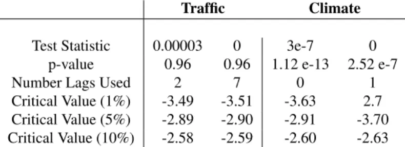
We also perform a DickeyFuller test in order to test the null hypothesis of whether a unit root is present in an autoregressive model. The test statistics of the traffic and climate data is shown in Table4, which demonstrate the non-stationarity of the time series.
Traffic Climate
Test Statistic 0.00003 0 3e-7 0
p-value 0.96 0.96 1.12 e-13 2.52 e-7
Number Lags Used 2 7 0 1
Critical Value (1%) -3.49 -3.51 -3.63 2.7 Critical Value (5%) -2.89 -2.90 -2.91 -3.70 Critical Value (10%) -2.58 -2.59 -2.60 -2.63
Table 4.Dickey-Fuller test statistics for traffic and climate data used in the experiments. .4. Prediction Visualizations
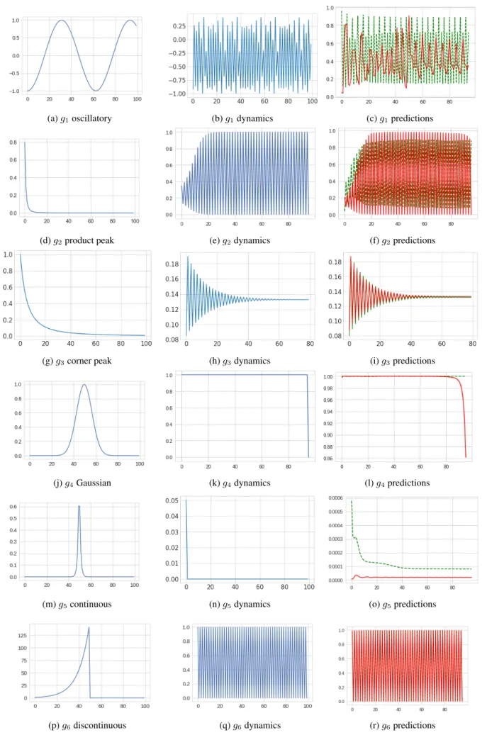
Genz functions are basis functions for multi-dimensional Figure10visualizes different Genz functions, realizations of dynamics and predictions from TLSTM and baselines. We can see for “oscillatory”, “product peak” and “Gaussian ”, TLSTM can better capture the complex dynamics, leading to more accurate predictions.
(a)g1oscillatory (b)g1dynamics (c)g1predictions
(d)g2product peak (e)g2dynamics (f)g2predictions
(g)g3corner peak (h)g3dynamics (i)g3predictions
(j)g4Gaussian (k)g4dynamics (l)g4predictions
(m)g5continuous (n)g5dynamics (o)g5predictions
(p)g6discontinuous (q)g6dynamics (r)g6predictions
Figure 10.Visualizations of Genz functions, dynamics and predictions from TLSTM and baselines. Left column: transition functions, middle: realization of the dynamics and right: model predictions for LSTM (green) and TLSTM (red).
.5. More Chaotic Dynamics Results
Chaotic dynamics such as Lorenz attractor is notoriously different to lean in non-linear dynamics. In such systems, the dynamics are highly sensitive to perturbations in the input state: two close points can move exponentially far apart under the dynamics. We also evaluated tensor-train neural networks on long-term forecasting for Lorenz attractor and report the results as follows:
Lorenz The Lorenz attractor system describes a two-dimensional flow of fluids:
dx dt =σ(y−x), dy dt =x(ρ−z)−y, dz dt =xy−βz, σ= 10, ρ= 28, β= 2.667.
This system has chaotic solutions (for certain parameter values) that revolve around the so-called Lorenz attractor. We simulated10 000trajectories with the discretized time interval length0.01. We sample from each trajectory every10units in Euclidean distance. The dynamics is generated usingσ= 10ρ= 28,β = 2.667. The initial condition of each trajectory is sampled uniformly random from the interval of[−0.1,0.1].
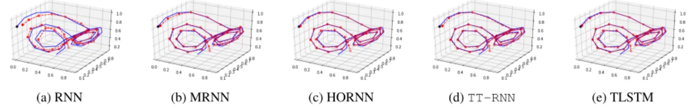
Figure11shows45steps ahead predictions for all models. HORNN is the full tensorTT-RNNusing vanilla RNN unit without the tensor-train decomposition. We can see all the tensor models perform better than vanilla RNN or MRNN. TT-RNNshows slight improvement at the beginning state.
(a) RNN (b) MRNN (c) HORNN (d)TT-RNN (e) TLSTM
Figure 11.Long-term (right 2) predictions for different models (red) versus the ground truth (blue).TT-RNNshows more consistent, but imperfect, predictions, whereas the baselines are highly unstable and gives noisy predictions.