Financing retirement consumption and bequests

(1)

Financing Retirement Consumption and Bequests

Tonja L. Bowen Bishop

M.S. Economics

Massachusetts Institute of Technology, 2008 B.A. Economics and American Studies

Brigham Young University, 2003 Submitted to the Department of Economics

in Partial Fulfillment of the Requirements for the Degree of Doctor of Philosophy in Economics

at the

Massachusetts Institute of Technology

MASSACHUSETTS INSTM OF TECHNOLOGY

OCT 20 2009

LIBRARIES

A ccepted by ...

...

Esther Duflo

Abdul Latif Jameel Professor of Poverty Alleviation and Development Economics

Chairman, Departmental Committee on Graduate Studies

(2)

Financing Retirement Consumption and Bequests

by

Tonja L. Bowen Bishop

Submitted to the Department of Economics

on August 14, 2009 in Partial Fullfillment

of the Requirements for the Degree of

Doctor of Philosopy in Economics

Abstract

This dissertation consists of three essays that evaluate possible vehicles for financing either retirement consumption or bequests. Chapter 1 compares the use of Roth and tax-deferred retirement accounts for retirement consumption with the use of taxable accounts. Previously, economists have often assumed that retirement savings should be done in a tax-deferred account. However, the advent of Roth-style tax-favored accounts and concerns about the tax implications of increasing retirement income through distributions from tax-deferred accounts warrant revisiting this question. I use data on married couples in the HRS and NBER's TAXSIM model to measure the probability of a household facing a higher tax rate at ages 62, 65, and 69 than the household faced at age 57. When the marginal tax rate is higher, the household could decrease their lifetime tax burden by choosing a Roth-style account over a tax-deferred account. I also measure the probability of facing a marginal tax rate that is sufficiently high that the household minimizes tax payments by using a taxable account rather than a tax-deferred account, when a Roth option is not available. I find that for distributions beginning at age 69, between 10 and 35% of households with taxable income at age 57 should prefer a Roth account to a tax-deferred account, but very few households prefer a taxable account.

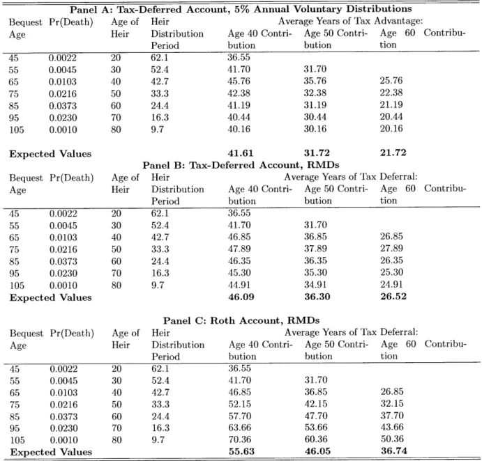
Chapter 2 models the tax-savings available through the use of tax-favored retirement accounts for bequests. Past research on tax-favored retirement accounts has focused on the incentives and effects of these accounts within the framework of the life-cycle model. However, tax-favored accounts also offer substantial tax savings for bequeathed assets. This chapter examines the incentives tax-favored accounts provide for bequests and simulates models of the available tax savings. The benchmark model calculates that the tax savings associated with a tax-deferred account (TDA) that is used to optimally bequeath assets exceeds the tax savings of a TDA used to produce a steady stream of retirement income by by 27.2%. Use of a Roth account for a bequest increases tax savings by an additional 32% over a bequeathed TDA.

(3)

of financing retirement consumption. Housing wealth is the most important non-pension wealth component for many elderly homeowners in the United States. Reverse mortgages allow elderly homeowners to consume housing wealth without having to sell or move out of their homes. Though the U.S. reverse mortgage market has grown substantially, very few eligible homeowners use reverse mortgages to achieve consumption smoothing. This chapter examines all Home Equity Conversion Mortgage (HECM) loans originated between 1989 and 2007 and insured by the Federal Housing Administration (FHA). It shows how characteristics of HECM loans and HECM borrowers have evolved over time, compares borrowers with non-borrowers, and analyzes loan outcomes using a hazard model. In addition, it conducts numerical simulations of HECM loans originated in 2007 to illustrate how the profitability of the FHA insurance program depends on factors such as termination rates, housing price appreciation, and the schedule of payments. This analysis serves as a starting point in understanding the implications of recent growth in the reverse mortgage market. Our results also suggest caution in predicting the profitability of the current HECM program.

Thesis Supervisor: James M. Poterba Title: Mitsui Professor of Economics

(4)

Acknowledgments

This thesis would not have been written without the support of my advisor, Jim Poterba. He drew me into the field of Public Finance by putting me to work as a research assistant after my first year at MIT. Jim then led me through the minefield of choosing a topic, con-sistently offered insightful feedback on my research efforts, helped secure financial support, and encouraged me to keep going when I encountered roadblocks. His belief in me gave me reason not to give up on myself.

I have also benefited from the comments and support of my second advisor, Peter Diamond. He has helped me understand how to fit the questions studied in this thesis into a larger economic context. Many other professors at MIT contributed to my economic education as I took classes and shared casual conversations. Helpful comments on this work were offered by Steve Venti (at Dartmouth), Amy Finkelstein, Bill Wheaton, and many participants in the MIT Public Finance lunches and seminars. I especially thank Dan Feenberg of NBER for his help with the implementation of TAXSIM and Mohan Ramanujan for facilitating my access to HRS restricted data.

In addition, I have benefited from association with a fabulous group of peers since arriving at MIT. Hui Shan was my office buddy both at MIT and at NBER, and my work has benefitted greatly from the insights she offered as a colleague and coauthor and the encouragement she gave as a friend. Discussions with Neal Bhutta, Chris Smith, Amanda Kowalski, and others to numerous to mention also contributed to the development of these papers.

Financial support for the early years of my studies at MIT came through an MIT Presidential fellowship, economics department graduate fellowships, and teaching assistantships. Later years were supported by the National Institute of Aging, Grant Number

T32-AG000186-i

~~--'

'i;~l i'i'-ll-^---.-i---i-~ii^iiiii;--\i ,-~;;--~il~-~~Tr*--i~-l-r--~ ;r^_---

_

~_?

--

L^~ir;ir.~.-;~-,,~

-r-~x

(5)

18 to the National Bureau of Economic Research, and by the Bradley Fund at MIT. In my last year, I have worked as a Research Associate at the Federal Reserve Bank of Boston, and am grateful for the support of my supervisors, Paul Willen and Chris Foote, as I com-pleted this dissertation. The conclusions reached in this paper are solely my own and do not represent opinions or policy of MIT, NBER, NIA, the Federal Reserve, or the Federal Government.

I also wish to remember those that inspired me to pursue graduate studies in eco-nomics. At BYU, Jim McDonald was incredibly generous with his time and encouragement as I deliberated my future plans. Kerk Phillips and Mark Showalter offered me my first experiences in statistical programming and data management when I worked as an under-graduate research assistant. Many other faculty members served as friends and mentors: Val Lambson, Arden Pope, Lars Lefgren, and Scott Bradford deserve particular mention.

Finally, I wish to thank my family for the support they have offered before and during my time at MIT. From a young age, my parents taught me to value education and strive to excel. They have offered a listening ear and nonstop encouragement, and have always let me know that they are proud of my efforts. I thank my sister Meesa for moving across the country with me and helping me adjust to life on the east coast, but more particularly for being a great friend and cheerleader for so many years. I thank my brothers, Jamon, Derrick, and Tyson, for their support, for the political discussions, and for the laughter that we have shared. And to Rob, thanks for valuing my endeavors, for pushing me when I have felt discouraged, for accepting no excuses, and for making me laugh when I needed it most.

(6)

2.5.1 Duration of Tax-favored Treatment . . . . 2.5.2 Magnitude of Potential Tax Savings . . . . 2.6 Conclusion . . . . ... . . . . 61 . . . . 64 . . . . 66 . . . . 68 . . . . 70 . . . . 73 . . . . 75 . . . . 78 . . . . 79 . . . . 81 . . . . 85

3 Reverse Mortgages: A Closer Look at HECM Loans (joint with Hui Shan)

3.1 Introduction ... 3.2 Background ...

3.2.1 Review of Existing Studies . .. ... 3.2.2 Background on the HECM Program . . . . . . . . .. 3.3 Data Description ...

3.4 Analysis of HECM Borrowers and Loans . . . . . . . . . .. 3.4.1 Changes in HECM Borrower and Loan Characteristics . . . .

3.4.2 Comparison of HECM Borrowers with the Overall Population of El-derly Homeowners ...

3.4.3 Termination Outcomes of HECM Loans . . . . . . . . .... 3.5 Simulation of HECM Program Profits . ... . . ...

3.5.1 HUD Insurance Pricing Model . . . . . . . . ..

3.5.2 Simulation Model ... 96 96 99 99 103 110 111 111 113 115 116 116 118

(8)

3.5.3 Simulation Results ... ... . 121

3.6 Conclusion ... ... .. ... .. 125

Bibliography 144

(9)

List of Figures

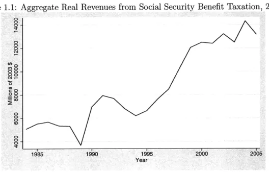
1.1 Aggregate Real Revenues from Social Security Benefit Taxation, 2003 $ . . . 44

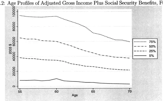
1.2 Age Profiles of Adjusted Gross Income Plus Social Security Benefits, Full Sample 45 1.3 Age Profiles of Taxable Income, Full Sample . ... 45

3.1 MCA and Appraised Housing Value . ... .... 128

3.2 Median Expected Interest Rate Charged on HECM Loans and Ten-Year

Trea-sury Rates ... . ... ... . 128

3.3 Calculating the Principal Limit . ... . . . . 129 3.4 Distribution of HECM Borrower Gender and Marital Status by Loan

Origi-nation Year ... . 130

3.5 Distribution of Monthly Payments for HECM Loans Originated in 2007 that

Have a Term or Tenure Component . ... .. 130

3.6 Growth in HECM Loans 1989-2007 .. ... . . . . 131

3.7 Growth in Indebtedness among Homeowners Aged 62 or Above 1989-2004.. 131 3.8 Distribution of HECM Borrower Age by Loan Origination Year ... 132 3.9 Distribution of Real House Values by Loan Origination Year . ... 133 3.10 Distribution of the Initial Principal Limit (IPL) to House Value Ratio by Loan

Origination Year ... . 134

(10)

3.12 Termination Hazard Rates of HECM Loans for Single Males, Single Females,

and Couples . ... ... 135

3.13 Termination Rates of HECM Borrowers and Survival Probabilities of the

Gen-eral Population ... ... 136

(11)

List of Tables

1.1 Characteristics of Types of Tax-Favored Accounts . ... 46

1.2 Value of Tax-Favored Accounts ... ... 47

1.3 Summary Statistics ... . ... . . . 48

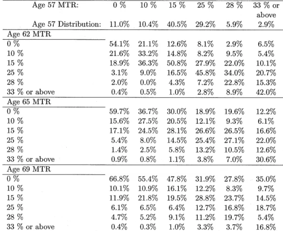
1.4 Marginal Tax Rate Distributions at Selected Ages . ... 49

1.5 Distributions of First Dollar Marginal Tax Rates by Age 57 MTR ... 50

1.6 First Dollar Preferences for Roth or Taxable Accounts Over Tax-Deferred Accounts ... ... . ... ... 51

1.7 Sample with Tax-Deferred Accounts: Distributions of Last Dollar Marginal Tax Rates by Age 57 MTR ... ... . 52

1.8 Sample with Tax-Deferred Accounts: Last Dollar Preferences for Roth or Taxable Accounts Over Tax-Deferred Accounts . ... 53

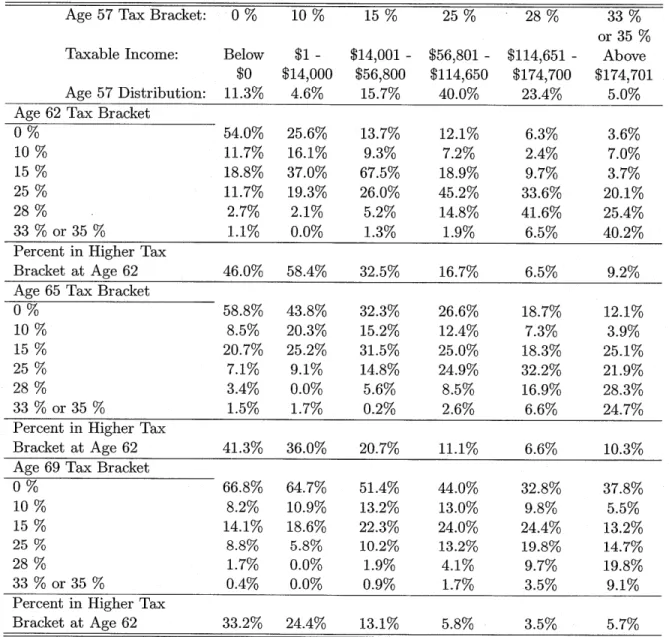
1.9 Distributions of Taxable Income by Age 57 Tax Bracket . ... 54

1.10 Selected Household Characteristics, by Age and Sample . ... 55

1.11 Distributions of Social Security Taxability: Households Receiving Social Se-curity Benefits ... ... ... ... . 56

2.1 Distribution Period for Use by IRA Owners . ... 87

2.2 Single Life Expectancy for Use by IRA Beneficiaries . ... 88

(12)

2.4 Flow of IRA Bequests, 2004 ... . ... 90 2.5 Duration of Tax Advantage for Contributions to Tax-Favored Accounts . . . 91 2.6 Expected Years of Tax-Deferral for Various Cases, Contribution at Age 50 92 2.7 Savings Associated with Tax-Favored Bequests .. ... 93 2.8 Expected Tax Savings of Tax-Deferred Bequests, Selected Parameters . . . . 94 2.9 Expected Tax Savings of Tax-Favored Bequests, Selected Circumstances ... 95

3.1 HECM Payments for a Hypothetical Borrower ... ... 137 3.2 Median Age and House Value of HECM Borrowers and Elderly Homeowners

in Survey of Consumer Finances . ... ... . ... . . 138 3.3 Characteristics of Zip Codes with and without HECM Loans .. . ... 138 3.4 MSAs with the Most HECM Loans Originated between 1989 and 2007 . . . 139 3.5 Proportional Hazard Model Estimation Results . ... 140 3.6 Fraction of Loans Resulted in Claims due to Foreclosure, Assignment, and

Lower-than-Expected Sale Price . . . . ... ... ... 140 3.7 Simulation Results on HECM Loans Originated in 2007: Probability of HUD

Insurance Claim and Average Claim Amount . ... .. . . .. 141 3.8 Simulation Results on HECM Loans Originated in 2007: Average

Profits-per-Loan for HUD ... . . ... . 142

3.9 Simulation Results on HECM Loans Originated in 2007: Costs to Borrowers 143

(13)

.-Introduction

This thesis consists of three essays that evaluate vehicles for financing either retirement consumption or bequests. The first two chapters consider two types of tax-favored retirement accounts: tax-deferred accounts, in which contributions are tax-deductible, accruals are not subject to taxation while remaining in the account, and distributions from the account are taxed as ordinary income; and Roth accounts, in which contributions are made with after-tax dollars, but neither accruals within the account nor distributions from the account are subject to taxation. The third chapter, which is joint work with Hui Shan, considers a very different potential source of funding for retirement consumption: extracting equity from a primary residence through a reverse mortgage.

Economists have often assumed that to the extent possible, retirement savings should be done in a tax-deferred account. However, the advent of Roth-style tax-favored accounts and concerns about the tax implications of increasing retirement income through distribu-tions from tax-deferred accounts warrant a revisiting of this question. Specifically, Gokhale, Kotlikoff, and Neumann (2001) shows that for some low-income households, taking distribu-tions from a tax-deferred account can raise the degree to which Social Security benefits are taxable, such that this additional taxation swamps the benefit of the tax-deferral. In Chap-ter 1, I use data on married couples in the HRS and NBER's TAXSIM model to measure the probability of a household facing a higher tax rate at ages 62, 65, and 69 than the household

(14)

faced at age 57. When the marginal tax rate is higher, the household could decrease their lifetime tax burden by choosing a Roth-style account over a tax-deferred account. I also measure the probability of facing a marginal tax rate that is sufficiently high that the house-hold minimizes tax payments by using a taxable account rather than a tax-deferred account, in the absence of a Roth option. I find that for distributions beginning at age 69, between 10 and 35% of households with taxable income at age 57 should prefer a Roth account to a tax-deferred account, but very few households prefer a taxable account. This chapter is a revised and expanded version of my MIT Masters thesis.

Past research on tax-favored retirement accounts has focused on the incentives and effects of these accounts within the framework of the life-cycle model. However, many house-holds hope to leave a bequest, and tax-favored accounts also offer substantial tax savings for bequeathed assets. Chapter 2 examines the incentives tax-favored accounts provide for bequests and simulates models of the available tax savings. The simulation focuses on the savings associated with the differential tax treatment of tax-favored accounts under the as-sumption that marginal income tax rates are constant over time. The benchmark model calculates that the tax savings associated with a tax-deferred account (TDA) that is used to optimally bequeath assets exceeds the tax savings of a TDA used to produce a steady stream of retirement income by by 27.2%. Use of a Roth account for a bequest increases tax savings by an additional 32% over a bequeathed TDA.

Housing wealth is the most important non-pension wealth component for many el-derly homeowners in the United States. Reverse mortgages allow elel-derly homeowners to consume housing wealth without having to sell or move out of their homes. However, histor-ically very few eligible homeowners have used reverse mortgages to smooth consumption in retirement. To encourage the development of the market for reverse mortgages, in the late 1980s the Federal Housing Administration (FHA) initiated a program of insuring a

stan-'~'-;'r--- --

-;I;;i--r rr;.-;---_-

ilrr;-x....~_~.~;-i^rra;r~r--urrr~-~n_.

.r - ---

r-n-r^;r;i--^o---

-- -r..;

(15)

dardized reverse mortgage products known as Home Equity Conversion Mortgage (HECM) loans. The final chapter analyzes HECM loans and simulates models of the profitability of the FHA insurance program. It shows how characteristics of HECM loans and HECM borrowers have evolved over time, compares borrowers with non-borrowers, and analyzes loan outcomes using a hazard model. The numerical simulations on HECM loans originated in 2007 illustrate how the profitability of the FHA insurance program depends on factors such as termination rates, housing price appreciation, and the schedule of payments. This analysis serves as a starting point in understanding the implications of recent growth in the reverse mortgage market and suggests caution in anticipating the profitability of the current

(16)

Chapter 1

Variation in Marginal Tax Rates

Around Retirement and the Return

to Saving in Tax-Favored Accounts

1.1

Introduction

Since the 1980s, the US has moved from a pension system dominated by defined benefit (DB) plans, pensions that pay out an annual benefit based on the worker's final salary and years of service, to one dominated by defined contribution (DC) plans, such as 401(k) plans.1 _This change has attracted much attention from economists, as the switch exposes plan participants to a very different set of risks than the previous regime. In addition, plan participants must make a number of decisions that previously were made for them by plan administrators, such as how much to save, how to invest the assets, and how quickly to consume their wealth in

1

See Buessing and Soto (2006), Clark and McDermod (1990), Gustman and Steinmeier (1992), Ippolito

(1995), Kruse (1995), and Papke (1999).

(17)

-retirement. One decision that has not received much attention is the choice of what type of account to use for retirement savings. This is in part because conventional wisdom has been that the answer is straightforward: workers at a firm offering a 401(k) or similar plan should take advantage of the tax-favored treatment of these accounts.

In recent years, this answer has become unsatisfactory for two reasons. First, the 2006 advent of Roth 401(k) plans, in which contributions are subject to taxation but then ac-crue gains tax-free, as an alternative to traditional tax-deferred 401(k)s, with tax-deductible contributions and taxable distributions, means that this answer is incomplete. When both options are available, a worker must decide how to allocate her retirement savings across tax treatments. Secondly, a recent paper by Gokhale, Kotlikoff, and Neumann (2001), argues that using a tax-deferred 401(k) may not be advantageous for all households. For those with low retirement income, taking distributions from a tax-deferred account can raise the degree to which Social Security benefits are taxable, such that this additional taxation swamps the

benefit of the tax-deferral. This means that when only a tax-deferred 401(k) plan is available,

some lower income workers are better off saving for retirement in a taxable account outside of the plan if there is no increase in compensation associated with participation.

This paper seeks to shed light on the decision of the type of account to use in saving for retirement by investigating the patterns of taxation facing married households as they age, using data on income and other determinants of taxation from the Health and Retirement Study (HRS), and making use of the TAXSIM program of the National Bureau of Economic Research (NBER) to calculate the marginal tax rate on a dollar contributed to or distributed from a tax-deferred account.2 When comparing Roth and tax-deferred savings accounts, the

after-tax value of an equivalent investment depends only on the marginal tax rate (MTR)

faced at the time the tax is levied, either at contribution or at distribution. Similarly, I will

2

(18)

later show that the value of access to a tax-preferred account can be expressed in terms of the MTR associated with such an account that would yield the same after-tax balance as a regular taxable account. Thus MTRs at different ages are a sufficient statistic for the factors that make various savings vehicles more or less attractive to a household seeking to maximize consumption. I find that a substantial minority of households, between 10% and 35%, face lower marginal tax rates at age 69 than at age 57, suggesting that Roth accounts should be an important part of retirement planning. In contrast, very few households face high enough marginal rates to recommend choosing a taxable over a tax-deferred account.

The paper proceeds as follows. The next section reviews the related literature on tax-favored accounts and retirement savings, and section 3 provides background informa-tion on tax-favored savings accounts and Social Security benefit taxainforma-tion. Subsequently, I describe my data and the TAXSIM program used to calculate MTRs. I also describe the sample used in my analysis and changes in income sources as my sample ages. In the fifth section, I investigate the question of how often the marginal tax rate faced at the time of withdrawal from a tax-favored account exceeds the rate faced at the time of contribution, and how often the marginal rate is enough higher to imply that a tax-deferred account would be dominated by a fully taxable account. This is accompanied by a discussion of the charac-teristics associated with higher marginal rates in old age. The penultimate section considers strategies that a household might employ to minimize tax costs resulting from tax-deferral, and the final section concludes.

1.2

Literature Review

Buessing and Soto (2006) reports a shift in the pension landscape between 1981 and 2003. In 1981, more than eighty percent of workers covered by a pension plan had DB coverage,

(19)

and perhaps a quarter of these had a DC plan as well. In contrast, by 2003, more than sixty percent of pension covered workers depended solely upon a DC plan. Other work on this transition suggests that in the early eighties, the increase in DC plan coverage was mostly due to shifting employment patterns and the addition of supplemental DC plans, rather than a switch away from DB plans by established companies.3 However, in later years, Papke (1999) finds evidence of firms substituting away from DB plans toward DC plans. By the early two thousands, firms with both types of plans were less likely to offer the traditional pension plan to new workers, and in some cases DB plan benefits were frozen at the accrued value for all workers at the firm.4 Also, since the early nineties, cash balance plans have expanded significantly as many firms convert traditional DB plans to this new type of pension, nominally a DB plan but accruing value in a way that mirrors DC plans.5

One of the early questions raised by the proliferation of tax-deferred savings accounts was whether such accounts represent new savings or simply a transfer of existing assets or planned savings to the tax-favored vehicle. The debate is summarized in Engen, Gale and Scholz (1996) and Poterba, Venti and Wise (1996). Essentially, Engen, Gale and Scholz

(1996) argue that much of the balance in Individual Retirement Accounts (IRAs) is not

likely to represent new savings, but Poterba, Venti and Wise (1996) counter that much of the balance of 401(k) plans consists of savings that would not have been done without the availability of such plans. Engen and Gale (2000) then suggests that the proportion of 401(k) contributions that represent new savings varies by earnings level.

Another important question raised by the transition from DB to DC pensions is

3

See Clark and McDermod (1990), Gustman and Steinmeier (1992), Ippolito (1995), and Kruse (1995).

4

See Munnell and Soto (2007).

5_{See Coronado and Copeland (2004), D'Souza, Jacob, and Lougee (2008), and Beussing and Soto (2006).}

Cash balance conversions from traditional DB plans were common in the mid and late nineties, as such a switch offered significant tax advantages over a switch from a DB to a DC plan. However, popular and legal controversy, including congressional hearings in 1999 and 2003, slowed the stream of conversions for a while. The rules and status of cash balance pension plans were normalized by the Pension Protection Act of 2006.

(20)

how the risk profile facing workers has changed. Bodie, Marcus and Merton (1988) discussed the different types of risks faced by participants in either type of plan, but data was not brought to this issue until more recent years. Samwick and Skinner (2004) use data on DC and DB plans from the Survey of Consumer Finances, along with synthetic earnings histories, to compare the present discounted value (PDV) of wealth accumulations under each regime. They find that for many workers, DC plan accumulations are likely to exceed the PDV of DB plan benefits. Schrager (2005) studies a similar question using the Panel Study of Income Dynamics, and finds that increasing job turnover in the nineties has made DC plans relatively more attractive to workers. Poterba, Rauh, Venti and Wise (2007) use the HRS to simulate DB and DC plan balance distributions for each household and find that although DC plans yield a higher PDV than private-sector DB plans, they are also more likely to generate very low retirement balances.

Recently a few papers have investigated the question of how to optimally make use of the available vehicles for retirement savings. As mentioned previously, it had generally been assumed that tax-favored accounts are the optimal means of accumulating retirement wealth. However, Gokhale, Kotlikoff and Neumann (2001), shows that for low-income households, making maximum contributions to a tax-deferred account could theoretically increase the lifetime tax burden by triggering the taxation of Social Security benefits. Butricia, Smith and Toder (2008) also investigate how benefit taxation affects retirement income. In addition, Kotlikoff, Marx and Raphson (2008) considers the question of whether a tax-deferred or Roth account is preferable under different assumptions about future tax regimes. My paper differs from these because I use actual earnings histories from the HRS rather than simulated earnings histories, allowing me to observe stochastic variations in earnings paths over time. In addition, I can calculate the percentage of households that have earnings such that they could be exposed to the Social Security benefit taxation trap exposed by Gokhale, Kotlikoff and Neumann (2001). My paper is also unique in that I consider the optimality of using

20

(21)

~i~-tax-favored accounts both when a Roth option is and is not available, and that I focus on the choice of savings vehicles when the household is already close to retirement age, when beliefs about the future evolution of the tax code are less important than at younger ages.

1.3

Institutional Background

1.3.1

Value of Tax-favored Accounts

Currently, the US tax code allows for many types of tax-favored accounts. Some of the most common include traditional Individual Retirement Accounts (IRAs), tax-deferred 401(k)s and similar accounts, and Roth versions of both IRAs and 401(k)s. Table 1.1 summarizes key aspects of the different types of accounts, and further details of the history and characteristics of these accounts are described in the appendix. The results in this paper abstract from the details of the many different types of tax-favored accounts available and consider three generic savings vehicles, denoted as a taxable account, a tax-deferred account, and a Roth account. All of the accounts have the same investment opportunities. The taxable account is funded with after-tax dollars, and accruals are taxed annually at a constant rate,6 with no tax due when money is withdrawn from the account. Contributions to the tax-deferred account are tax-deductible, no tax is levied on accruals within the account, and distributions are taxed as ordinary income as long as the account holder has reached the age of 59 1. The Roth account differs in that contributions are not deductible, but distributions of both the principal and any accrual are non-taxable after age 59 1.

6

Actual taxation of capital income depends on whether the income is received as interest, dividends, or capital gains. Applying a constant tax rate that is independent of the tax rate on income is most similar to current tax treatment of qualified dividends, and represents an intermediate case between the tax treatment of interest, taxed as ordinary income, and the tax treatment of capital gains, which are taxed at a constant rate only upon accrual.

(22)

Tax-deferred and Roth accounts are considered tax-favored because they eliminate the taxation of income from assets held in such accounts. More explicitly, a pre-tax contri-bution of C made at time 0 and held in a taxable account that accrues value continuously at a pre-tax rate of r for T periods will yield the following balance at time T, with the con-tribution taxed at the marginal ordinary income rate that applies in time 0, t9, and capital income taxed each period at the constant rate tr:

balancetaxable = (1 - t°)Cer(1-tr)T

Holding funds in a tax-deferred account (TDA) causes three changes: it eliminates the tax on capital income, eliminates the income taxability at time 0, and causes the full balance to be taxed whenn is withdrawn in time T at the marginal ordinary income rate tT, yieldingit the following after tax balance:

balanceTDA (1

tT)CerT

In contrast, holding funds in a Roth account only eliminates the capital income tax, but does not change the timing of income taxation. The following equation describes the bal-ance:

balanceRoth (1 t)CerT

Thus, if the tax rate is constant, the tax-deferred and Roth accounts are equivalent, although the reported balance in a tax-deferred account will appear larger because taxes have not yet been levied. Both have a higher after-tax balance than a taxable account facing the same marginal income tax rate because they avoid capital income taxation. Some examples are shown in Table 1.2; the first column shows the ratio of the pre-tax contribution to the after-tax balance for a after-taxable account facing different marginal rates, assuming a capital income

I

1

___~_iiil (__llii~---il_~ ._I.ll--_~~-t-_l.---iXI

-;(i_---li-=~F;I

ii^~i----iiii

..-.-

(23)

_--tax rate of 15%, a nominal interest rate of either 6 or 10%, and a holding period of either five or twelve years.7 The second column shows the same ratio for a Roth or tax-deferred

account associated with a given marginal rate.

From these equations and the table, it is clear that for any MTR, the Roth account will be preferred to the taxable account. Similarly, the choice between tax-deferred and Roth accounts is straightforward, and depends only on the marginal income tax rates that apply at the time of contribution and withdrawal of the funds. If the marginal rate is higher at the time of contribution, the tax-deferred account is preferred, but if the marginal rate is higher at the time of distribution, the Roth account will be preferred. Comparing the taxable account with the tax-deferred account is slightly more difficult when the tax rate can change over time. For example, table 1.2 shows that for either a five or twelve year holding period and a 6% nominal interest rate, a tax-deferred account facing a marginal rate of 28% or above is inferior to a taxable account facing a rate of 15% or less. However, if the interest rate is 10%, the taxable account with a 15% rate is preferred to the tax-deferred account with a 28% marginal rate only for the five year holding period. For the twelve year holding period, the benefit of tax-deferral compensates for the higher marginal rate on this account. More generally, one can solve the above equations for the tax rate that would cause the tax-deferred account to yield the same balance as the taxable account:

t = 1- (1 - ti)/e'

For any ty greater than tT*, the taxable account will be preferred to the tax-deferred account, and for any tT less than tT *, the tax-deferred account will be preferred. The tT* that

7

A 6% return roughly corresponds to the average nominal annual return on a diversified portfolio of bonds, and a 10% rate to the return on large-cap equity. According to the 2005 SBBI Yearbook, the compound annual total return for term government bonds was 5.4% from 1926 to 2004, 5.9% for long-term corporate bonds, and 10.4% for large company stock. A five year holding period corresponds to the time between ages 57 and 62, and a twelve year holding period corresponds to the time between ages 57 and

(24)

corresponds to a given t9 is presented in column three of Table 2. The above equation shows that tT * will be increasing in tP, r, tr, and T. Intuitively, this means that the benefits of

a tax-deferred account are increasing with respect to the available return on capital, the marginal rate of capital taxation, and the intended holding period of the asset. Thus if an individual is choosing between taxable and tax-deferred accounts with given marginal tax rates, a higher return on capital or a longer holding period will make the tax-deferred account more attractive.

As noted in the introduction, conventional wisdom has been that the lack of labor income in retirement causes marginal tax rates to be lower in retirement, or at least not higher than in previous years, so tax-deferred accounts should be the optimal retirement savings vehicle. Roth accounts are only recommended early in the lifecycle of those that expect relatively high tax rates in retirement, or perhaps for those that expect an increase in statutory rates in the future. However, there is little evidence that marginal rates in retirement are relatively low: first, because we know little about the paths of income before and after retirement, and secondly because the complexity of the tax code, especially the phasing in and out of various provisions, means that higher incomes do not always correspond to higher MTRs. For example, Gokhale, Neumann, and Kotlikoff (2001) finds that lower income households could experience reduced lifetime consumption and higher lifetime tax-bills as a result of fully participating in a tax-deferred 401(k) because of increased taxability of Social Security benefits. This result can be linked to high MTRs associated with the phase-in of Social Security benefit taxability.

1.3.2

Social Security Taxability

As a response to long-term concerns about the viability of the Social Security program, the Social Security Amendments of 1983 enacted several provisions to restore solvency to the

(25)

system over a seventy-five year horizon. Scheduled increases in the payroll tax rate were accelerated, the full benefit retirement age was set to gradually increase, and most relevant to the purposes of this paper, up to fifty percent of household benefit payments became subject to taxation, with revenues flowing into the Social Security trust fund. The income threshold above which benefits are taxable was set at $25,000 for single households, and $32,000 for those married filing jointly and was deliberately not indexed for inflation so that the taxability of benefits would be introduced gradually. Ten years later, further reform set a second threshold ($34,000 and $44,000, respectively), above which 85% of benefits become taxable.

To calculate the portion of Social Security benefits that are taxable, a household starts with its adjusted gross income (AGI) less Social Security benefits, and adds in several items exempted from AGI, most notably tax-exempt interest income. They then add half of their Social Security benefits and fill out a worksheet that compares this amount with the applicable thresholds. If the household's total is less than the first threshold, none of the Social Security income is taxable. If the household's total is between the two thresholds, the lesser of half the difference between the total and the threshold or half of benefits are taxable. If the total is above the second threshold, the household similarly transitions to 85% taxability. The phasing in to higher levels of benefit taxability occasions a jump in marginal tax rates. For example, if a household has income such that they are in the first transition range, an additional dollar of taxable income will cause another fifty cents of Social Security benefits to be subject to tax, so the effective MTR is 1.5 times the statutory rate. Similarly, in the second phase-in, the effective marginal rate is 1.85 times the statutory rate. The size of the transition range is directly linked to the amount of Social Security benefits received.

(26)

example, consider the case of a married household that has $18,000 in taxable income as well as Social Security benefits and a large tax-deferred account.8

In my HRS sample, average Social Security benefits for a household with a 65-year-old male are around $12,000. If the household takes no distributions from the tax-deferred account, or up to a $8,000 distribution, none of the Social Security benefits will be taxable. On the other hand, if the household takes a distribution from the account of $26,000, 85% of benefits, or $10,200, is taxable. If we assume that the household takes the standard deduction, they face a statutory MTR of 15%, so they pay an extra $1530 in taxes. This is equivalent to a 12.75% reduction in Social Security benefits. A distribution between $8,000 and $26,000 results in a lower tax penalty, but the transition into benefit taxation generates higher effective marginal rates, 22.5% and 27.75%. A second example is a household that receives the maximum possible benefit, about $28,000.9 In this case, any distribution from a tax-deferred account will trigger Social Security benefit taxation. Benefit taxability again reaches 85% with a $26,000 distribution, and the household faces the same 12.75% reduction in benefits, or a $3570 tax penalty. If the household's economic situation does not change, it may face such a penalty year after year.

Some twenty years after taxability of Social Security benefits was introduced, the fraction of households subject to the tax growing each year, as is the amount of revenue collected. In the 2000 HRS, about one third of households receiving Social Security income pay taxes on some portion of their benefits, and about one fifth have sufficient income levels that 85% of benefits are taxable. For married households with Social Security income, those numbers rise to one half and thirty-five percent. Nationally, revenues collected from Social

8

The numbers in this example were chosen to most clearly illustrate effect of Social Security benefit taxation, but are not unreasonable. $18,000 is slightly less than the average wage earnings of 69-year-old individuals in my sample, as reported in Table 1.3. Similarly, in Section 1.5.2, I report the average simulated

distribution from a tax-deferred account as just over $7,000.

9If both spouses claim benefits upon reaching age 65 in 2003 and each had earnings that exceeded the upper limit on Social Security taxation in each of the 35 previous years, household benefits are approximately

$28,000.

(27)

Security benefit taxation have grown steadily over time, from about five billion dollars in 1984 to more than twelve billion in 2006 (using constant 2003$), as shown in Figure 1.1. The increase in revenue can be attributed to three things: first, the lack of inflation indexing of the taxability threshold means that each year, more households are subject to a tax; second, because benefit levels are based on a formula that inflates wages by real wage growth rather than just inflation, real benefits are increasing over time; and finally, the addition of the second threshold in 1993.

1.4

Data Description

Data for this paper comes from the HRS, a biannual survey of elderly and near-elderly households starting in 1992. I construct variables for tax-filing status, dependents, age exemptions, taxable income sources, and deductions using the survey responses of married couples in the original HRS cohort from the 1992-2004 waves of the HRS, generally following the methods of Rohwedder, et al. (2005). This includes constructing mortgage interest paid as a percentage of reported mortgage debt, with the percentage reflecting the average annual interest rate paid on a 30-year loan as calculated by HSH Associates.1o I depart from the Rohwedder, et al. (2005) method by using data from the Social Security Administration

(SSA) on earnings and Social Security benefits. HRS asked respondents to give permission to access their earnings and benefits histories from the SSA in both 1992 and 2004. I make use of the benefits histories and two types of earning records provided by SSA that go back to 1980: w-2 earnings and Medicare covered earnings.1 1 Unfortunately, SSA data cannot be merged with any geographic data in the HRS, so I assume that all households are located in Massachusetts, following Gokhale, Kotlikoff, and Neumann (2001). Further,

10

See http://www. hsh. com/mtgst. html

1 1

The primary difference between these two measures of earnings is that w-2 earnings deduct contributions to tax-deferred accounts.

(28)

I face one issue that Rohwedder, et al. (2005) did not: distinguishing between qualified and unqualified dividend income. I assume that qualified dividends are a fixed fraction of total dividends, based on the numbers reported in the Statistics of Income for 2005.12 Finally, I use a variation of NBER's TAXSIM program to calculate the MTRS for the years the male member of the couple is or would be between the ages of 57 and 69, based on a uniform 2003 tax code and Social Security benefit taxability thresholds corresponding to their real values

in each year.

In many cases, implementing TAXSIM at younger ages requires the extrapolation of the values of input variables into the period before 1992. I have data on wages and Social Security benefits in prior years, but other income variables must be extrapolated. I assume that no unemployment insurance benefits are received, that dividends and other capital income, including interest, rental, and business income, remain constant in real terms, and that pension income starts at the age reported in the HRS and has a constant nominal value. Deductions must also be extrapolated; I assume that rent payments and property taxes remain constant in real terms, that charitable contributions are a constant, household-specific fraction of income, that there are no deductible medical expenses, and that outstanding

mortgage debt declines annually at a household-specific rate.

For my analysis, I choose to use a tax code that is constant except for one element: the Social Security benefit taxability thresholds decline in real terms over time because of the lack of inflation indexing. To accomplish this, I convert all values into 2003 dollars and let TAXSIM calculate the AGI that would pertain in the absence of Social Security income. I compare the AGI and the Social Security benefits received by a household to the applicable real threshold and calculate the portion of benefits that are taxable and whether benefit taxability is being phased-in. Then I add taxable benefits to ordinary income, rerun

12_{See Marcia and Bryan (2007).}

(29)

TAXSIM to get the MTR that applies to non-wage income, and multiply this marginal rate by the appropriate factor to account for the phasing in of benefit taxability."l To streamline my analysis, I consider only couples that are married at the time I begin my calculations, the year the male reaches age 57, and omit couples that experience a divorce during my sample period. In addition, I must make several sample restrictions due to data availability: both members of the couple must be alive in 1992 and linked to the SSA records, and the male must be born between 1926 and 1935. This range of birthdates leads to a sampld of couples with males ages 57 to 62 in 1992, allowing me to construct the needed variables for all ages between 57 and 69. The consequences of these sample restrictions on my sample size are as follows: there are 7648 households in the 1992 HRS cohort, 4545 of which are married both in 1992 and when the male is 57 years old. Further limiting the sample to couples with the male born between 1926 and 1935 results in 2380 households, and dropping those that experience a divorce leaves 2316 households. Of these, 1640 have SSA records for both

household members and make it into my sample.

Because I calculate MTRs over a twelve year sample period, the household may experience the death of one or both members. In the case of a widow(er), the household files as single and faces the resulting tax brackets. If both household members pass away, MTRs for subsequent years are coded as missing. To consider the effects of these sample composition choices, we can consider the sample of HRS married couples with the male aged 57 in 1992. In 2004 the male has reached age 69, and we find that 73.1% of these households

1 3

The 2003 tax brackets are as follows, according to the 1040 Instructions for 2003, available at http:

//www.irs.gov/pub/irs-prior/i1040--2003.pdf.

Marginal Tax Rate Single Married Filing Jointly 10% Below $7,000 Below $14,000 15% $7,001-$28,400 $14,001-$56,800 25% $28,401-$68,800 $56,801-$114,650 28% $68,801-$143,500 $114,651-$174,700 33% $143,501-$311,950 $174,701-$311,950 35% Above $311,950 Above $311,950

(30)

still survive as married couples. For 21.1% of households, only a widow(er) remains, and in 2.5% of households, both have passed away. Only 3.3% of couples have experienced a divorce after twelve years.

Summary statistics for the values of the variables that serve as inputs into TAXSIM are shown in Table 1.3, for both age 57 and age 67, with the full sample in Panel A. Through-out my analysis, households are weighted by their 1992 household weight. It is clear that as they age, households become less likely to receive wage and dividend income, and more likely to receive income from property, pensions, and Social Security. In addition, at age 67, households are less likely to be eligible to take tax-deductions for property tax payments, mortgage interest payments, and charitable donations.14 _{A drop in average wages for} pri-mary earners15 _{at age 67 suggests that many may only work part-time later in life, however,} the increase in average secondary wages implies that lower earning women may be less likely to remain in the labor force. The increase in average Social Security benefits both reflects that older couples are more likely to have both members claiming benefits and those who wait longer to claim benefits have larger benefits.

Panel B of Table 1.3 shows summary statistics for the sample of households that report holding a positive balance in a tax-deferred account in at least one wave of the HRS, a sample consisting of 1206 households. A comparison of these two samples suggests that households with tax-deferred accounts tend to have higher earnings at age 57 and more capital income at age 67, but are otherwise very similar. Households in this sample may be slightly more likely to receive various income types and be eligible for various deductions, but these differences are relatively small. Overall, these results suggest that households with tax-deferred accounts have larger lifetime incomes than others.

14Medical expense deductions are very close to zero at all ages.

15Primary earners are males in households with both members of the couple surviving, and of the surviving widow(er) otherwise.

(31)

As noted in the introduction, the expectation of lower tax rates in retirement is based on the idea that that taxable income will be lower after earnings have ceased. Although this seems a reasonable assumption, it has not generally been examined. Several papers have noted that since the 1970s, the economic status of the elderly has improved and the incidence of poverty has declined.16 This may indicate that the assumption of lower income in retirement is outdated. Indeed, Table 1.3 indicates that although both the probability and the level of earnings decrease between ages 57 and 67, other types of income increase simultaneously. In Figure 1.2, we can see that the profile of a broad income concept, AGI plus non-taxable Social Security benefits, declines at a surprisingly shallow rate. At age 70, the income levels at the 25th, 50th and 75th percentiles of the distribution are well over half of the income level at age 55, when earnings are near their lifetime peak. Although it is difficult to discern in the figure, income levels at the bottom of the distribution do drop significantly, and upon reaching age 70 are not much more than a third of the age 55 level.

Marginal tax rates depend not on this broad income measure, but on taxable income, which may exclude some Social Security benefits and capital income and also takes into account a tax exemption for the elderly and a myriad of deductions and credits. Figure 1.3 shows the profiles of taxable income for various quantiles, and all decline more significantly than did the broader income concept. This implies that over time, households shift from earned income to less heavily taxed sources of income, and may also reap greater benefits from tax deductions and credits. However, the idiosyncratic nature of this transition, particularly the differences in the timing of retirement by different households, may lead to "churning" within the distribution at a higher rate than during the working life. A comparison of the

MTRs facing individual households at different ages can better show the probability of facing high rates when taking distributions from a tax-deferred account.

16

(32)

1.5

Analysis of Marginal Tax Rates

1.5.1

First Dollar MTR

I first consider the question of how households should allocate their first dollar of retirement

savings. I use Medicare covered wages, supplemented by w-2 earnings when Medicare wages are not available, to determine the MTRs that apply before making any tax-deferred con-tributions. Throughout this section, actual MTRs are divided into bins corresponding to the statutory rates. Most of the marginal rates calculated by TAXSIM are tightly clustered around the statutory rates, but phase-ins and phase-outs of deductions and Social Security benefit taxation cause some outliers. In addition, the 33% and 35% bins are grouped together because of their low frequency. The distribution of MTRs faced at ages 57, 62, 65 and 69 are shown in Panel A of Table 1.4. As households age, the proportion of households facing lower MTRs increases, so that at age 69, almost one-third of households face a zero marginal rate and just over two-thirds face a marginal rate of 15% or less. However, the fraction of households facing a rate of 25% or more stays relatively stable around 10%, suggesting that a portion of the population may have an income profile that does not significantly decline with age.

Table 1.5 calculates the distribution of MTRs at ages 62, 65, and 69 by the marginal tax rate at age 57. Thus along the diagonals are the percentages of households facing roughly the same MTR, and below the diagonal the percentages of households facing higher marginal rates. In addition, Panel A of Table 1.6 summarizes the percentage facing higher rates at each age, or the percentage of households that would face lower discounted lifetime tax payments by taking the first dollar of their distribution from a Roth account rather than a tax-deferred account. At age 62, almost half of households facing marginal rates of 0 or 10% at age 57 are now facing higher rates, and 14 to 25% of households that faced rates of 15%

(33)

or more at age 57. At age 69, these numbers drop to around a third for households in the lowest age 57 bins, and to 10 to 19% for those facing higher marginal rates. This indicates that a non-trivial fraction of households would pay less in taxes by choosing Roth accounts instead of tax-deferred accounts, especially if they face low marginal rates at age 57 or plan to begin distributions relatively soon.

The second two panels of Table 1.6 show the percentages of households that would pay less in taxes by using a taxable account than by taking distributions from a tax-deferred account, for 6% and 10% nominal return on assets. These are the households with marginal rates at ages 62, 65, and 69 that are higher than the equivalent marginal rate for their age 57 tax rate, as explained in section 1.3.1. I first consider the case of a 6% annual return on assets. Among households facing age 57 marginal rates of 10% or less, upon reaching age 62, the fraction of households that prefer the taxable account is nearly as high as the fraction that prefer the Roth: between 45% and 50%. Households facing a 15% marginal rate also have only a slightly lower probability of choosing the taxable account, a drop from 25% to 22%. This lines up with Gokhale, Kotlikoff and Neumann's (2001) assertion that some low-income households may not realize a tax savings by using tax-deferred accounts. In contrast, households facing higher rates at age 57 are less likely to be better off using a taxable account: the fraction preferring a taxable account is 40 to 80% lower than the fraction preferring a Roth. However, by age 69, the fraction preferring the taxable account is much lower for all households facing positive marginal rates at age 57, and is less than 3% for those with an age 57 marginal tax rate of at least 25%. These overall patterns persist when a 10% nominal return is considered, though even fewer households prefer taxable accounts. By age 69 and with asset returns of 6 and 10%, only 11.5% and 3.3% of all households pay lower lifetime taxes by using a taxable account than by taking distributions from a tax-deferred account, and many of these faced a zero marginal rate at age 57. Thus households with longer savings horizons are unlikely to face a scenario in which taking retirement distributions from

(34)

a tax-deferred account is dominated by making use of a taxable account.

1.5.2

Sample with Tax-deferred Accounts: Last Dollar MTR

The preceding analysis reports the attractiveness of Roth and taxable accounts for the gen-eral population. However, those actively saving for retirement may differ from the gengen-eral population in significant ways, so looking at the change in MTRs for a sample of households with tax-deferred accounts may be more informative in ascertaining their optimal choice of savings vehicle. Additionally, for the subset of households that regularly makes contributions to a tax-deferred account and limited access to Roth savings, the relevant question may be whether the household should substitute some Roth savings for tax-deferred savings. Thus for this portion of my analysis, I use only households that report having a positive balance in a tax-deferred account in some wave of the HRS and calculate the MTR that corresponds to the last dollar of the contribution made or distribution taken. This allows me to discover how many households would have been better off by replacing some of their tax-deferred savings with savings in some other type of account. I use wages as reported on w-2 forms rather than Social Security wages to account for possible tax-deferred contributions to 401(k)s during the working life. Additionally, I calculate simulated distributions from tax-deferred accounts at ages 62, 6 5 and 69 as a fraction of the reported or interpolated balance in the account in that year, setting that fraction equal to the ratio of the number of members of the couple still alive to the sum of their life expectancies. The simulated distribution is not subtracted from the remaining account balance, so at each age, my analysis implies an assumption that distributions begin at that age at a rate that is sustainable for the remaining life expectancy of the couple. The size of the average simulated distribution is $7,138 and does not vary greatly with age. In my sample, distributions are small relative to other income sources. Be-cause tax-deferred accounts have only become widely available in the 1980s and my sample

i

;_~___i__:l_____l__l~_l_____sln___rl~_ ____j

iiil;-iii-I-lii-_I(~I

li-~~--i---i--l---l(_11-~I~

Il^--iil~i-lil^

1;

liiiiiiiiiii;i~i

-I~iiii~l*ll~O~i-i-l--^-~

IC~__^l~_ili--l

i---~^-miiil

~.L_

i(--I^l^l-*-~i-;ili---

-ii-~-ir~--ii

(35)

reached age 62 by 1997, households have not had as many years to accumulate tax-favored savings as future cohorts will. Thus my calculations should be taken as conservative esti-mates of the impact of taking tax-deferred distributions on last-dollar marginal tax rates in retirement.

Again, Table 1.7 calculates the distribution of MTRs at ages 62, 65, and 69 by the MTR at age 57, and Panel A of Table 1.8 summarizes the percentage facing higher rates at each age, or the percentage of households that could lower their discounted lifetime tax payments by taking the last dollar of their distribution from a Roth account rather than a tax-deferred account. These results follow the same patterns evident in the first dollar MTR results for the full sample, though the fraction of the population preferring a Roth is larger, especially for those facing very low MTRs. This suggests that among those facing very low marginal rates, households with tax-deferred savings accounts are more likely to face a low rate only temporarily, perhaps due to unemployment or unusually large deductions. At age 62, roughly three-quarters of households with marginal rates of 0 or 10% at age 57 are now facing higher rates, and at age 69, about half these same households would have preferred a Roth account. Among households facing rates of 15% or more at age 57, only 16 to 32% experience higher rates at age 62, and 9 to 28% at age 69. This indicates that many current holders of tax-deferred accounts would pay less in taxes had they used Roth accounts in addition to tax-deferred accounts and taken a portion of their distribution from the Roth account.

In the second two panels of Table 1.8 are the percentages of households that would pay less in taxes by taking the last dollar of their distribution from a taxable account than from a tax-deferred account for a 6% and 10% nominal return on assets. Again, the results look very similar to the full sample results, but with slightly higher magnitudes. Among households facing age 57 marginal rates of 15% or less, upon reaching age 62, the fraction

(36)

of households that prefers the taxable account is only slightly smaller than the fraction that prefers the Roth account. In contrast, households facing higher rates at age 57 are less likely to prefer a taxable account than to prefer a Roth account. By age 69, the fraction preferring the taxable account is much lower for all households facing positive marginal rates at age 57, and is less than 5% for those with an age 57 marginal tax rate of at least 25%. Similar patterns emerge when a 10% nominal return is considered, but even fewer households prefer taxable accounts. By age 69 and with nominal asset returns of 6 or 10%, only 14% and 3.5%, respectively, of all households in the sample would pay lower lifetime taxes by using a taxable account than by taking distributions from a tax-deferred account.

1.5.3

Understanding Increases in Marginal Tax Rates

As we have seen, though few households would prefer a taxable account to a tax-deferred account, a substantial minority is better off using a Roth account than a tax-deferred account because they face higher marginal tax rates later in life. Why might they face higher rates? As mentioned before, they may simply have more taxable income than previously, through some combination of full- or part-time earnings, capital income, pension benefits, and Social Security benefits. Table 1.9 shows the distribution of taxable income at ages 62, 65, and 69 into bins corresponding to the statutory rates, by the bin at age 57. This table differs from Table 1.7 in that it does not account for the impact of phase-ins and claw-backs on the actual marginal rates faced. It shows that for those with age 57 taxable income placing them in the 15% bracket or lower, increases in taxable income are responsible for nearly all of the increase in marginal tax rates at ages 62 and 65, and most of the increase at age 69. These might represent households that were unemployed or underemployed and returned to work, or households that had retired but were not yet receiving pension or Social Security benefits. For those with more substantial taxable income at age 57, increases in taxable income also

(37)

play a role in raising marginal rates, accounting for between half and all of the marginal rate increases at age 62, and between 35 and 60% of the marginal rate increases at age 69.

In thinking about increases in taxable income, it should be noted that households that are still working full time are unlikely to be taking distributions from retirement ac-counts, so increases for these households should not be a concern. Though retirement is notoriously difficult to measure, determining the presence of earned income for an individual is straightforward. Thus Panels A and B of Table 1.10 show the percentages of households at ages 62, 65, and 69 that still have one or both members of the couple earning income for various cuts of the data. Those facing higher marginal rates at later ages are much more likely to have one or both members of the couple still earning income. At age 62, more than 40% of households facing higher marginal rates have two wage-earners, and more than 80% have at least one wage-earner. By age 69, these percentages have dropped, but those with higher marginal rates are still much more likely to have earned income than is the population at large.

If taxable income has not increased for a household but the MTR has, two plausible reasons might be that the household has been widowed or that the household is experiencing a phase-in of Social Security benefit taxation. After a household is widowed, different tax brackets apply, so the same taxable income could trigger a much higher rate. However, Panel