University of Tartu
Institute of Mathematics and Statistics
Samuel Amankwaa
Singular points binomial method for pricing
American fixed lookback options
Masters thesis in financial mathematics
Masters (15 EAP)
Supervisor Toomas Raus, University of Tartu
Singular points binomial method for pricing American fixed lookback op-tions
Abstract:An option is the opportunity to buy or sell an underlying asset with a fixed price at a given time in the future. One of the biggest difficulties in option theory is determining the correct value of an option. In this thesis, we discuss what European and American options are, we further move on to price American lookback options using the singular point method. We use singular points which are formed on the nodes of the tree and apply the binomial method to find price of the option which are represented as continuous piecewise linear functions. The reflection principle and combinatorics are used in pricing European lookback options. Under the re-flection principle the emphasis is on finding the appropriate probability convenient to use in pricing the option under the method suggested by John Hull. CERCS research specialisation:P160 statistics, operations research, programming, acturial mathematics.
Key words: financial mathematics, options, lookback options, binomial model, sin-gular points method.
Singulaarsete punktide meetod Ameerika tagasivaatavate optsioonide hin-damiseks
Lühikokkuvõte: Töös vaadeldakse tagasivaatavate (lookback) optsioonide hindamist. Tagasivaatavate optsioonide korral sõltub optsiooniga seotud väljamakse alusvara maksimaalsest või minimaalsest hinnast optsiooni eluajal. Töös vaadel-dakse binoommeetodil tuginevaid võimalusi nii Euroopa kui Ameerika tüüpi tagasi-vaatavate optsioonide hinna leidmiseks. Ameerika tüüpi tagasitagasi-vaatavate optsioonide hinna leidmiseks tutvustatakse töös singulaarsete punktide meetodit, mis on tundu-valt efektiiivsem võrreldes tavalise binoommeetodiga.
CERCS teaduseriala: P160 Statistika, operatsioonianalüüs, programmeerimine, finants- ja kindlustusmatemaatika.
Märksõnad: finantsmatemaatika, optsioonid, tagasivaatavad optsioonid, binoom-meetod, singulaarsete punktide meetod.
Contents
1 Chapter 1. Options 3
1.1 Options, option value . . . 3
1.2 The Black-Scholes formula . . . 5
1.3 Binomial model . . . 8
2 Chapter 2. Lookback options 13
2.1 Price of the European Lookback option . . . 13
2.2 Valuing American style lookback . . . 17 3 Chapter 3. Singular points method for American lookback options 20
3.1 Piecewise linear convex functions . . . 20
3.2 Pricing Lookback American options by singular points method . . . 21
3.3 Sketch of the algorithm of the singular points method . . . 25
3.4 Numerical examples . . . 26
List of references 27
IntroductionThis work briefly talks about option pricing , some basic termi-nologies used in option pricing which are covered in brief as it is not the main point of concern. It focuses on pricing lookback options using a modified algorithm of the binomial approach namely the singular point method. In this thesis, we discuss what European and American options are, which further move on to elaborate on using the binomial method which serves as a pivot in this thesis and contribute to this in use of the singular point method, to price American lookback options. This is a standard binomial technique for pricing by providing singular points at the nodes. Nothing changes much from the binomial method except the introduction of sin-gular points. The above is employed since we cannot find analytical formula for pricing lookback option. Even though Babbs[1] gives an accurate and efficient solu-tion to the problem for American and floating strike lookback by using a procedure of complexity of order 0(n2)by using a change of numeraire, this cannot be applied in the case of fixed strike price.
Nevertheless other possibilities are also catered for. For example the reflection principle and combinatorics are considered as alternatives in pricing European look-back options. The main concern here is to find the probability that the maximum or the minimum of the stock is greater or lesser than some security price levels.
For American options we consider singular points method but also looks at some technical notes from Hull for pricing American options.
In summary this thesis is divided into three parts namely- chapter 1 which deals with options and finding option values, chapter 2 which talks about path- de-pendent options with emphasis on lookback, asian and barrier options and finally chapter 3 on the use of the singular point method in pricing the American lookback options in addition to numerical analysis of sample results.
1
Chapter 1. Options
1.1
Options, option value
An option is the right but not the obligation , to buy or sell a security such as a stock for an agreed upon price known as the strike price for some time in the future known as theexercise time or expiry date. The right to buy a security is a call option and the right to sell a security is a put option[5]. We have the European and American type of options.
The European option is only exercised at maturity, the final time T . The value of the option at the final timeT can also be called the intrinsic value. Hence anEuropean call optionallows itsholderthe right (not obligation) to buy from the
writer a prescribed asset for a prescribed price at a prescribed time in the future. Mathematically the payment of the call option is given by max(S(T)−K,0)and that of the put is max(K −S(T),0)with S(T) being the price of the underlying security at final timeT[3]. The figure 1.1 highlights the payoff of the European call and put options
An American option its like the European option except that it can be exer-cised at any time between the start date and expiry date by its holder.
An American call option gives its holder the right(but not the obligation) to purchase from the writer a prescribed asset for a prescribed price at any time be-tween the start date and specific expiry date in the future. In the time interval[0, T]. Whereas an American put option gives its holder the right(but not the obli-gation) to sell to the writer a prescribed asset for a prescribed price at any time between the start date and specific expiry date in the future. In the time interval [0, T].
The price of an option today should replicate its future value at time T else there is an arbitrage opportunity and this should not exist on the market for a longer time before there is a movement in prices to eliminate them. Otherwise investors may take advantage and buy what is cheaper and sell at a higher price. Loosely we say "there is no such thing as "free lunch". Formally, opportunities to make instantaneous risk-free profit do not exist[2].
We also have the Put-Call parity. This is an argument between the relationship between the value of C of the European call and the value P of the European put option, with the same strike priceKand expiry dateT. We consider two portfolios πA: one call option plusKe−rT andπB :one put option plus one unit of the asset.
At expiry, the portfolioπAis worthmax (S(T)−K,0) +Kwhich can be written as
is also max (ST, K). If these two portfolios have the same value at expiry, we assume there is no arbitrage, then att= 0can say that the portfolios must have the same value at time0, and
C+Ke−rT =P +S(T) (1.1)
This relationship which connects the call and put options is theput-call par-ity[2].
The argument behind (1.1) can be made more precise via the no arbitrage principle. If πA is worth more thanπB at time0then it would be possible to sell
πA(that sell the call option and borrow the cash) and buyπB (that is buy one put
and one share). There is an instantaneous profit ofπA−πB(since we are sure that
the payoff ofπB compensates for that of πAat expiry). Such instantaneous profits
violates the no arbitrage principle. A similar argument holds if πB is worth more
thanπAat time zero[2].
1.2
The Black-Scholes formula
We look at the Black-Scholes formula which is very important in option pric-ing. The evolution of stock is governed by
∆S =µ·S∆t+σ·S·∆W(t). (1.2)
The ratio ∆SS gives the return on the asset price andµis the trend on the market andσ is the volatility. The quantityµ·S∆t is known as the deterministic part and σ·S·∆W(t)as the random part. The variableW is a stochastic variable (Brownian motion). The Variable ∆W(t) causes the uncertainty in the history of the stock price. The mean of W is 0 as intuitively wiggles up and down. Its variance over time T is stillT. The higher the σ the higher the "jaggedness" of the path of the asset price.
AWiener processalso known as the Brownian motion is a particular type of
Markov stochastic process . The behavior of the variable, W, which results from a Wiener process is ascertained by considering the changes in its value in small intervals of time. We consider a small interval of time of length∆tand let∆W be the change inW during∆t. We have the basic properties as follows.
Property 1. The quantity∆W must satisfy the equation ∆W =√∆t
where is a random variable generated by the standardized normal distribution N(0,1).
Property 2. The values of ∆W for any two short intervals of time are inde-pendent. That means the intervals of time do not overlap.
The assumption that the value of the underlying security follows a geometric Brownian motion implies that
S(t) = S(0)·exp(µ−σ2/2)·t+σ·∆W(t). (1.3) with all parameters as explained previously.
We make the following assumptions
• The stock price follows the log-normal distribution
• There are no taxes or transaction costs associated with hedging portfolio. • Trading of the underlying asset takes place continuously.
• There are no dividends during the life of the option on the underlying assets. If dividends are known before hand this assumption can be dropped. They can be paid either at discrete intervals or continuously over the life of the option. • There are no risk-less arbitrage opportunities. The absence of arbitrage
op-portunities means that all risk-free portfolios must earn the same return. • The risk-free rate of interest,r, and the asset volatilityσare known functions
of time over the life of the option.
• Short selling is permitted and the assets are divisible. We assume we can buy and sell any number(not necessarily an integer) of the underlying asset,and that we sell the assets we do not own.
Ifσ = σ(t)andr = r(t), then in partial differential senseV = V(S(t), t), the price of the option with stock priceS should satisfy the equation
∂V ∂t + 1 2S 2σ2∂2V ∂S2 +rS ∂V ∂S −rV = 0, S >0and0≤t < T.
This is known as the backward parabolic type if the final condition at time T is known and we solve backwards to find the price of the option else it is known as the forward parabolic type.
Without restrictions on the boundaries of the region which we solve for the value of the option price, a partial differential equation can have many different solutions. The domain of the unknown function V is a region in(S, t)-space. For
a European call option the value at timeT in the interval[0, T]is of interest andT is noted as the exercise time of the option. The domain of finding the value of the option price is
Ω ={(S, t)|0≤S < ∞and0≤t≤T}.
At timet=T the value of the security will either exceed the strike price and the call option will be exercised with a payoff of S(T)−K > 0or the security will attain a value less than the strike price, in this case the option expires unused and has no value. WhenS(T) > K the call option is said to bein the money. The call option out of the moneywhenS(T)< K. Thus the terminal value of the European call is
(S(T)−K)+ = max (S(T)−K,0).
where S(T) is the value of the underlying security at the exercise timeT and K is the is the strike price of the option. Hence, if Crepresents a price of European call option, we can write the following equation as the final condition for the Black-Scholes PDE:
C(S, T) = (S(T)−K)+.
At the boundary atS = 0, the call option is never exercised and has a value of zero. Thus we have one boundary condition namely
C(0, t) = 0.
Supposedly, ifS is approaching infinity, it becomes likely that the call option will be exercised asS→ ∞, it will exceed any finite value of K asKbecomes less and less important. AsS → ∞, hence the value of the option becomes that of the asset price and we write
C(S, t)≈S asS → ∞.
For a put option,with valueP(S, t), the final condition is the payoff P(S, T) = (K−S(T))+.
IfS is zero the final payoff is known with certainty to beK. To determine P(0, t) we have to calculate the present value of an amountK received atT. Assuming that interest rates are constant we find the boundary condition atS= 0to be
P(0, t) =Ke−r(T−t). More generally, for a time-dependent interest rate we have
AsS → ∞the option is unlikely to be exercised and so (see [10]) P(S, t)→0asS → ∞.
We assumeC denotes the European call price, and P denotes the European put price. The BS formula follows:
C=S(0)N(d1)−Ke−rTN(d2), P =Ke−rTN(−d2)−S(0)N(−d1) (1.4) where d1 = log(S(0)/K) + (r+σ2/2)T σ√T , d2 = log(S(0)/K) + (r−σ2/2)T σ√T ,
N(x)- cumulative normal probability,
σ2 - annualized variance of the continuously compounded return on the stock,
r- continuously compounded risk-free rate, T - time to maturity . Note: S0 =S(0) and N(x) = √1 2π Z ∞ −∞ e−y 2 2 dy .
1.3
Binomial model
For American options and exotic options (lookback options) we cannot find analytical formula for the price of the option and we must use some numerical method. In general there are three methods for finding the price:
• Binomial or trinomial methods • finite difference methods • Monte-Carlo method
In this work we consider mainly the binomial method as the basic method in option pricing.
It serves as an alternative to partial differential equation solution to Black-Scholes equation. It was initially developed by Cox, Ross, and Rubeinstein [Cox et.
Figure 1.2: Binomial model
Al. (1979)] popularly known asCox-Rox-Rubeinstein modelwhich is again called the lattice model[6]. A graph of a double time step lattice model is shown in fig 1.0. It serves as an alternative model to the Blacks-Scholes equation in finding prices of option values. We make the following assumptions in the derivation
• K is the strike price of the call option • T is the exercise time of the call option • S0, the initial price of the security
• r, the continuously compounded risk -free rate
• The price of the security follows a geometric Brownian motion with drift µ andσas in (1.3)
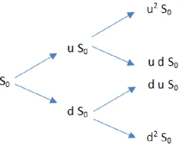
Suppose the time interval [0, T] is partitioned into n equal subintervals of length ∆t = Tn. In the binomial model it is assumed that if the asset price is S at time-stepn∆t, then it can either jump up to a higher valueuS, u >1with proba-bilitypor down to a lower valuedS, d <1with probability1−p. Here we assume the the parametersp, u, anddare constants and do not depend on time. Thus,
St+1 =
(
uStwith probabilityp
dStwith probability1−p
(1.5) We assume a risk-neutral world in which the underlying random walk for S is lognormally distributed. Then we can approximate this continuous random walk
with a discrete random walk having the same mean and variance. Hence if the underlying security can take on only values uStanddSt with probabilities p and
1−prespectively then after a time step of length∆twe have
puSt+ (1−p)dSt=Ster∆t. (1.6)
And finally leads to
pu+ (1−p)d=er∆t. (1.7) for allt. As var(St+1) = E(St2+1)−(E(St+1))2, then var(St+1) = St2(pu 2+ (1−p)d2−(pu+ (1−p)d)2). Finally we have pu2+ (1−p)d2 =e2r∆t+σ2∆t. (1.8) By now we have written the probability p as a function of r and ∆t and we have (1.8) which relatesuanddtor, σ, and∆t[8].
We can solve (1.7) as p= ue r∆t−1 u2−1 where d= 1 u (1.9)
With (1.8) and (1.9) we can write p= e r∆t−d u−d = σ2∆t+e2r∆t−d2 u2−d2 and hence u+d= 1 d +d= σ2∆t+e2r∆t−d2 er∆t−d
This is a quadratic expression ford, and toO(∆t32)its solution is given by the expressions p= e r∆t−e−σ√∆t eσ√∆t−e−σ√∆t (1.10) u=eσ √ ∆t, d=e−σ√∆t.
We may build up a lattice of possible asset prices. If at the current time t = 0we know the asset price,S0, then we divide the remaining life of the derivative security
set prices,uS0 anddS0. At the second time-step,2∆t, there are three possible asset
pricesu2S
0, udS0 =duS0 =S0andd2S0 = Su02.
In general, at the n-th time stepn∆t there aren + 1possible values of the underlying asset price,
dn−jujS0 =u2j−nS0, j = 0,1, ..., n.
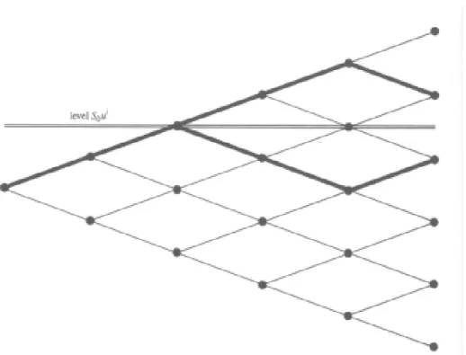
Note that in figure 1.2 the lattice reconnects and lends itself to two lessons.The first is that the history of a particular asset price is lost, as there is clearly more than one path to any given point. Thus path dependent options cannot be valued using this reconnecting lattices. Secondly the total number of lattice points increases only quadratically with number of time-steps. This implies a number of time-steps can be taken.
Assuming that we we know the payoff function for our derivative security and that it depends only on the values of the underlying at expiry, this enables us to value it at expiry, time-stepT =N∆T. If we consider a put, for example, we find that
PN,j = max(K−SN,j,0)andj = 0, ...N,
where PN,j denotes the possible values of the put at the final time T and the j-th
possible asset valueSN,j. For a call, we find that
CN,j = max(K −SN,j,0)forj = 0, ...N
whereCN,jdenotes the possible values of the call at expiry. We can find the expected
value of the option at the time-step prior to expiry,(N−1)∆t, and for possible asset priceSN−1,j, j = 0,1, ...N−1, since we know that the probability of an asset priced
atSN−1,j moving toSN,j+1 during a time step ispand the probability of moving to
SN,j is(1−p). Using risk-neutral argument we can find the value of the security at
each possible for time-step(N−1). Likewise this allows us to find the value of the security at time-step (N −2), and so on, back to time-step0. This is the value of the security at the current time.
With European options we consider the following. Let Vn,j be the value of
the option at time-step n∆tand asset price Sn,j(where0 6 j 6 n). We calculate
the expected value of the option at time step j + 1, given the asset priceSn,j, and
discounting this for the riskless interest rate,
er·∆TVn,j =pVn+1,j+1+ (1−p)Vn+1,j.
This gives
As we know the value ofVN,j, forj = 0, ...N option value at final timeT =N∆T,
from the payoff function we can recursively determine the values Vn,j for eachj =
0, ...nforn < N to arrive at the current value of the optionV0,0. We do not require
the asset pricesSn,j during the evaluation of the option prices butSN,j, when finding
VN,j. At each time-step we can discard the oldSn,j, as soon as we have foundSn+1,j.
OnceVN,j have been found, we can discardSN,j as well. This observation leads to
2
Chapter 2. Lookback options
According toDesmond J.Higham (2005)[2], the pay-off path dependent op-tions depends on path of the underlying asset occuring within the time interval. Examples are Barrier options, Asian options and Lookback options.
The payoff of the lookback option depends on the maximum or minimum price of the underlying asset occurring over the life of the option. The option allows the holder to "look back" over time to determine the payoff. There exist two kinds of lookback options: with floating strike and with fixed strike. We assume K is the fixed strike price andMT is the maximum value the underlying asset attains andmT
the minimum value in [0, T]. Hence the fixed lookback call and put can be priced in the following ways (MT −K)+ and (K − mT)+ respectively. Now we
em-phasise on the strike price K which attains the minimum value of the asset price, mT or the maximum value, MT giving way to a call or put respectively,hence we
have(ST−mT)+and(MT−ST)+and this is known as the floating strike lookback.
Another type of the path dependent options is the Asian options. This is de-termined by average case behaviour. We take a look at this
An average price Asian calloption has the pay-off at the expiry dateT given by max 1 T Z T 0 S(τ)dτ −K,0 .
There is also the barrier option which has a payoff that switches on or off depending on whether the asset price crosses a pre-defined level. We have two types namely the down -and- out call option anddown -and- in call. The former has a payoff that is zero if the asset crosses some predefined barriersL < S0, H > S0 at
some time interval[0, T]. If the barrier is not crossed then the payoff becomes that of the European call,max{ST−K,0}, ifL < St< H, t∈[0, T]. Whilst the latter has
a payoff zero unless the asset price crosses some predefined barrierL < S0,H > S0
at some time interval[0, T]. If the barrier is crossed then the payoff becomes that of the European call,max{ST −K,0}, ifL < St< H, t∈[0, T]
2.1
Price of the European Lookback option
Price of the European lookback option in the binomial model can be found using combinatorics and the reflection principle. First we consider the general idea about the reflection principle before considering how it can be used with the bi-nomial method to price lookback options. Now we look at the reflection principle based on the binomial theorem for option pricing as suggested by Stanley R. Pliska
Figure 2.1: The reflection principle
(1979) [9]. We define the binomial security price model withT periods which fea-tures the the four parameters;p, d, u, andS0, where
0≤p≤1,0≤d≤1≤u
and in factS0 >0. At timetthe price of the security is given by
St =S0uNtdt−Nt, t = 1,2...T.
, whereNt is the number of ’up’ moves. The probability distribution ofStis given
by P(St=S0undt−n) = t n ! pn(1−p)t−nn= 0,1, ...t
The binomial model can be used to compute the probability distribution for the maximum value achieved by the security process during the T periods. We derive this for the special case whered =u−1 and this leads to the simplified version
St=S0und2Nt−t
YT = max{St:t = 0,1, ...T}, and this random variable takes theT+1values
S0, S0u, ...S0uT. We want to compute P{YT > S0ui fori = 1,2, ...T}. Fixi, we
notice thatSi > S0ui if and only if2Nt−t >iso thatP{YT >S0ui}is the same
asP{2Nt−t > ifor somet}. The latter is computed with thereflection principle
as illustrated in figure 3.2. The main idea to find the first passage timeτ1 ≡min{t:
2Nt−t = i}, whereτ = ∞if2Nt−t < ifor allt 6 T, and take into account
all the sample paths for whichτ1 6 T. It follows then that there are three mutually
exclusive events. Ifiis one of the valuesT, T −2, T −4, ..., then it is possible to have the values 2NT −T = i,in this case τ1 6 T. Secondly, it is likely to have
τ1 < T and2NT −T > i. Thirdlyτ1 < T and2NT −T < i. Thus
P{YT >S0ui}=P{2Nt−t>ifor somet} (2.1)
P{YT >S0ui}=P{event1}+P{event2}+P{event3} (2.2)
The first probability is written as
P{event1}=P{NT = (T +i)/2}= T T+i 2 ! p(T+i)/2(1−p)(T−i)/2 The above holds if T +i is an even number else P{event1} = 0. For the second probability, if2NT −T > i, then definitelyτi < T, where 2NT −T is the
index ofuat the final timeT . Thus we have P{event2}=P{NT >(T +i)/2}= T X n=n∗ T n ! pn(1−p)T−n
wheren∗ is the smallest integer strictly greater than(T +i)/2. The sum is zero if n∗ > T. To compute the third probability is a bit challenging therefore we use the reflection principle. Under the reflection principle, each sample path in event 2is paired with a unique sample in event3as in figure 2.1. The sample paths coincide up toτi, and then each is the mirror image of the other across the leveli. Hence the
number of sample paths in the two events2NT −T > iand2NT −T < iare equal,
although their probabilities are not equal unlessp= 1/2.
To complete the computation of event3, we consider an arbitrary sample path from event 2, and suppose it is such thatNT =n(6 n∗). This sample path occurs
with probability pn(1−p)T−n and there are T
n
!
sample paths with NT = n.
Now looking at figure 2.1 it becomes apparent that "partner" of this sample path terminates withNT =T +i−n, a symmetric distance below the level(T +i)/2.
"partner" sample path ispT+i−n(1−p)n−i. Since there are T
n
!
sample paths in event3withNT =T +i−n, it follows that
P{{event3 ∩ {NT =T +i−n}}= T n ! pT+i−n(1−p)n−i in which case P{event3}= T X n=n∗ T n ! pT+i−n(1−p)n−i Hence finally, we have
P{YT >S0ui}= T T+i 2 ! p(T+i)/2(1−p)(T−i)/2+ T X n=n∗ T n ! [pn(1−p)T−n+ pT+i−n(1−p)n−i] At this point we have in principle, the probability distribution for the max-imum security price during T periods. Generally these formulas can be used for maximum security price during the first t periods whent < T. Since the event {Y >S0ui}is the same as the event{T 6t},we get the probability distribution for
the first passage time to security price levelsS0ui. Same procedure can be used for
the probability distributions of the minimum security price and the the first passage time to security price levels belowS0
There are exact formulas but if we use the binomial method, then we can find the price of the option usingcombinatorics(using reflection principle)
V(S, t) =e−r(T−t) n X i=0 P(YT =S0ui) max{S0ui−K}. Att= 0we have V(S,0) =e−r(T) n X i=0 P(YT =S0ui) max{S0ui−K},
whereP{YT =S0ui}is obtained from (2.3). We observe thatS0uias the maximum
stock price attained and the above equation for the price of the option is the Fixed Strike European Call Lookback option.
A similar argument can be used to price the the Fixed strike European Put option by takingYT to be minimum security price attained and its first passage time
2.2
Valuing American style lookback
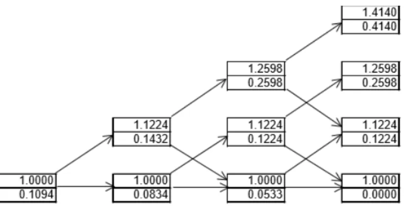
Moreover number of researchers have suggested various approaches to valu-ing lookback options. John Hull (1993)provides one of such possibilities we can use to price an American -style lookback put. We consider a security with initial stock price 50, with volatility 0.04, risk-free interest rate is0.1and the time to ex-piry is 3 months. We assume that three steps are used to model the stock price movements.
When the option is exercised, there is a payoff equal to the excess of the maximum stock price over the current stock price. Therefore we defineG(t)as the maximum stock price achieved up to timetand we set
Y(t) = G(t) S(t).
We move on to use Cox,Ross, and Rubinstein tree for the stock price to pro-duce a tree for Y. Initially, Y = 1 as G = S as time t = 0. If there is an up movement bySduring the first time step bothGandSincrease by the proportionu and the ratioY is still1. Mathematically we have
G(t+ 1) = max{S(t), S(t+ 1)} S(t+ 1) =uS(t) hence G(t+ 1) =uS(t) and Y(t+ 1) = G(t+ 1) S(t+ 1) Y(t+ 1) = 1.
Again if there is a down movement in the stock priceS,Gwill stay the same andY(t+ 1) = 1d =u. The rules for defining the geometry of the tree are
• WhenY = 1at timet, it is eitheruor1at timet+ ∆t.
• WhenY =um at timetform>1, it is eitherum+1 orum−1 at timet+ ∆t.
An up movement in Y relates to a down movement in the stock price, and vice versa. The probability of an up movement inY is1−p, where as a down movement isp. We value the American lookback option in units of stock price rather in dollars. In dollars the payoff is
This is valid asSY is the maximum price attained up to timet. Algebraically SY producesG, the maximum price attained and is fixed.
Whilst in stock price units the payoff is Y −1.
We roll back through the tree in the usual way, valuing a derivative that pro-vides this payoff except that we adjust for the differences in the stock price (i.e., the unit of measurement) at the nodes. Iffij is the value of the lookback
at thejthnode at timei∆tandYij is the value ofY at this node, the rollback
procedure gives
fij = max(Yij −1, e−r∆t[(1−p)fi+1,j+1d+pfi+1,j−1u])
Figure 2.2: Procedure for valuing an American-style lookback options
we note thatfij is to projected tofi+1,j+1 by multiplyingfi+1,j+1 bydand to
fi+1,j−1by multiplyingfi+1,j−1 byu
Similarly, whenj = 0the roll back procedure gives
fij = max(Yij −1, e−r∆t[(1−p)fi+1,j+1d+pfi+1,ju]).
As usualfi,0dandfi,juare option price values formed at the edges of the binomial
tree. At j = 0,Yij is the same for all i. This is because there is no change inS0
whatsoever and hence the ratio of G(t)toS(t) does not change. The solution to example is shown the following diagram above.
3
Chapter 3. Singular points method for American
lookback options
This chapter deals singular points method for American lookback options. In the binomial (Cox-Ross-Rubinstein) model, the price at timet = 0of the Amer-ican lookback option is given byV(0, S0, S0)where the functionsV(i, x, y)can be
computed by the following backward dynamic programming equations: V(n, x, y) =ψ(x, y)
V(i, x, y) = max(ψ(x, y), Vc(i, x, y)
Vc(i, x, y) =e−r∆T[pV(i+ 1, xu,max(xu, y)) + (1−p)V(i+ 1, xd, y)], whereψ(x, y)is the payoff function and u, d, pare the parameters of the binomial model. The valuation of V(0, S0, S0) requires a number of computations of order
O(n3).
Here we consider a general framework for pricing European/American lookback options in a efficient way. The main idea of the singular points method is to give a continuous representation, at each node of the tree, of the option prices as a piece-wise linear convex function of the path-dependent variable (maximum/minimum). These functions are characterized just by a set of points, which are called as "singu-lar points". All such functions can be evaluated by backward induction in a straight-forward way.
3.1
Piecewise linear convex functions
Definition 1. Given a set of points :(x1, y1), ...,(xn, yn), such thata=x1 <
x2 < ...xn=band yi−yi−1 xi−xi−1 < yi+1−yi xi+1−xi , i= 2, ...n−1, (3.1)
let us consider the function f(x), x∈[a,b] obtained by interpolating the given points linearly. The points (x1, y1), .., .(xn, yn), which characterise the piecewise linear
functionf are called the singular points off, whilex1, ...xnwill be called singular
values off.
Remark 1We considered only piecewise linear functions with strictly increas-ing slopes in the previous definition, hence the resultincreas-ing function is convex.
From henceforth only piecewise linear functions that are continuous and con-vex on the interval [a, b]are taken into account. A set of singular points for these functions are found and they must satisfy (3.1).
Lemma 1Let f be a piecewise linear and convex function defined on the inter-val[a, b]and letC = {(x1, y1), ...,(xn, yn)}be the set of its singular points. If we
remove a point(xi, yi)with2≤ i ≤n−1, from the setC, the resulting piecewise
linear function f, whose set of singular points is C\{(xi, yi)}, is again convex in
[a, b]and we have
f(x)≤f(x), x∈[a, b] .
Proof. The convexity of f follows from the fact that function f is the maxi-mum between f and the function given by the straight line joining the points(xi−1, yi−1)
and(xi+1, yi+1).
Remark 2. It follows from Lemma 1 that every piecewise functionf whose singular points are a subset ofC (containing the first and the last singular points) is still convex and satisfiesf(x)> f.
Lemma 2. Let f be a piecewise linear and convex function defined on [a, b]
and let C = {(xi, yi)}, i = 1, ..., n be the set of its singular points. We denote
(x, y), the intersection between the straight lines joining (xi−1, yi−1),(xi, yi) and
the one joining(xi+1, yi+1),(xi+2, yi+2),2≤i≤n−2. If we consider a new set of
n−1singular points{(x1, y1), ...,(xi−1, yi−1),(x, y),(xi+2, yi+2), ...,(xn, yn)}, the
associated piecewise functionf is convex on[a, b]andf(x)≤f(x), x∈[a, b].
Proof. The singular points of f satisfy the property of increasing slopes (3.1). The set of slopes of f are obtained by removing the slope of the line join-ing(xi, yi),(xi+1, yi+1), hence (3.1) is again satisfied andf is convex.
3.2
Pricing Lookback American options by singular points method
Now we describe the singular points method for fixed strike American look-back call option. The method consists in valuating the price of the option, at each node of the tree, for each possible choice of the maximum at that point. In the bi-nomial model Let us denote byNi,j the node of the binomial tree whose underlyingasset price is Si,j = S0u2j−i, i = 0, ..., n, j = 0, ...,1. To each node Ni,j we will
associate a set of singular points, whose number isLi,j. The singular point will be
denoted by
(Mi,jl , Pi,jl ), l = 1,2, ..., Li,j.
The singular valuesMi,jl are called singular maximums andPi,jl are called singular prices. At first we need to find the maximum and minimum values of the maximum Ml
n,j underlying stock in the American case at the nodes Nn,j, j = 0,1, ..., n. It
follows that the maximum varies between a minimum valueMmin
valueMn,jmax, where
Mn,jmin = max (Sn,j, S0), Mn,jmax =S0uj.
For each M ∈ [Mmin
n,j , Mn,jmax]the price of the option can be continuously defined
by Vn,j(M) = (M −K)+. The function Vn,j(M) is a piecewise linear function
satisfying Definition 1, whose singular points are valuable in a straightfowrard way. In fact:
• ifK ∈(Mmin
n,j , Mn,jmax)then the price value functionVn,j(M)is characterised
by the 3 singular points(Ml
n,j, Pn,jl ), l= 1,2,3(henceLn,j = 3), where
Mn,j1 =Mn,jmin, Pn,j1 = 0; (3.2) Mn,j2 =K, Pn,j2 = 0; (3.3) Mn,j3 =Mn,jmax, Pn,j3 =Mn,jmax−K. (3.4) Note:P1
n,j = 0is as a result of max (Mi,jmin−K,0) = 0andPn,j2 = 0is obvious.
• IfK /∈(Mn,jmin, Mn,jmax)then price value function Vn,j(M)is characterised by
the 2 singular points(Ml
n,j, Pn,jl ), l= 1,2(henceLn,j = 2), where
Mn,j1 =Mn,jmin, Pn,j1 = (Mn,jmin−K)+ (3.5)
Mn,j2 =Mn,jmax, Pn,j2 = (Mn,jmax−K)+. (3.6)
• In the case j = 0andj = nthe minimum and maximum ofM coincide and Ln,j = 1.
Lemma 3. At each node at maturity,the functionVn,j(M) that provides the
price of the option, is a piecewise linear function on the interval (Mmin
n,j , Mn,jmin).
Moreover,such function is convex on its domain.
Consider now the step i,0 ≤ i ≤ n −1. At the node Ni,j we can evaluate
recursively the minimum and maximum value of the maximumM of the underlying by the relations
Mi,jmin = max (Mimin+1,j+1/u, S0), Mi,jmax =M max i+1,j.
Lemma 4. At each node Ni,j, i = 0, ...n, j = 0, ..., i, the functionVi,j(M),
which provides the price of the option as function of the maximumM, is piecewise linear and convex in the interval[Mmin
Proof. The claim is true at step i = n (at maturity by Lemma 3). Con-sider the step i = n − 1. We extend the function Vi+1,j+1(M) to the interval
[Mimin+1,j+1/u, Mimax+1,j+1] and we take Vi+1,j+1(M) = Vi+1,j+1(Mimin+1,j+1) for M ∈
[Mmin
i+1,j+1/u, Mimin+1,j+1]. With such an extension the continuation value price
func-tionVi,jc(M), becomes
Vi,jc(M) = e−r·∆T[pVi+1,j+1(M) + (1−p)Vi+1,j(M)]. (3.7)
The price of an American lookback option can be obtained by computing only the singular points of the price function at each node. The structure of the tree in the lookback case gives us the opportunity to evaluate the singular points of Vi,j in an
efficient way. The procedure is elaborated in an ensuing Proposition 1 to be tackled soon. Hence we need to have some properties relating to the lookback case:
Lemma 5. The price value function Vi,j(M), M ∈ [Mi,jmin, Mi,jmax] has the
following properties:
a) ifK ∈[Mi,jmin, Mi,jmax]thenVi,j(M)is constant in[Mi,jmin, K],
b) ifM ∈[Mmin
i,j , Mi,jmax−1]andVi,j(M) = M −KthenVi,j−1(M) = M −K, c) ifM ∈[Mimin+1,j+1, Mi,jmax]andvi+1,j+1(M) = M−K thenvi,j(M) =M −K,
d) assume thatx1 =S0ul, x2 ∈ (S0ul, S0ul+1),x3 = S0ul+1 are singular values of
Vi,j. If we delete the singular point(x2,Vi,j(x2))thenV0,0(S0)does not change. Proof. Properties(a)and(b)follows backward induction on the tree. Property (c)follows from(b)and we can conclude from(c)that, at the nodes Ni+1,j+1 and
Ni,j the same function passes through the singular points at those nodes.
The claim of property(d) follows by the fact that the value of the option at the nodesNi,0, Ni,i,i= 0, ..., n−1, depends on the values assumed byVi+1,j at the
nodes of the tree.
Again by Lemma 5(d), we deduce that every singular value which lies be-tween consecutive nodal stock values and which are singular values as well, can be removed. This means the critical valueMi,j can be removed, during the backward
iterations without affecting the price of the option if it lies between two consecutive nodal values.
In the ensuing proposition we shall get to know that the set of internal singular points of vi,j at each node can be reduced to a set of consecutive singular nodal
values which are singular values ofvi,j well as noted earlier, with the final addition
ofK.Mi,j lies between two consecutive nodal singular values and it can be ignored
in the backward iteration by Lemma5(d).
Proposition 1 Consider the price value function Vi,j and denote by l0 the
smallest integer l such that S0ul > max(K, Mi,jmin). The set of singular values of
Vi,j can be reduced to :Mi,jmin, Mi,jmax, K if K ∈(Mi,jmin, Mi,jmax)and a set
singular values of Vi+1,j+1 as well. Moreover if M = S0ul0+k <
Mmax i,j
u , then
Vi,j(M) =M −K.
Proof. Consider the casei = n−1. We take firstj ≥ int[2i]andj < n−1 (the case j = n − 1 is trivial). At the node Ni,j, the singular values of Vi,jc are
Mmin
i,j , Mi,jmax, K if K ∈ [Mi,jmin, Mi,jmax] and eventually uMi,jmin = Mimin+1,j+1. By
Lemma 5(a) uMi,jmin is a singular value of Vi,jc if and only ifuMi,jmin is greater or equal thanK.
Now we consider the function Vi,j. The singular values ofVi,j are the same
ofVc
i,j and with possible addition ofMi,j (critical values) if it exists. IfMi,j exists
then more importantly uMi,jmin is a singular value and K < uMi,jmin. By Lemma 5(c)Vi,j(uMi,jmin) = uMi,jmin −K sinceVi+1,j+1(uMi,jmin) = uMi,jmin −K. We can
then conclude thatMi,j ∈ [Mi,jmin, uMi,jmin]and by Lemma5(d)it can be removed.
Hence the claim holds.
In the casej < int2ithere are no singular values in(K, Mi,jmax)so the claim is trivial.
Now we consider the general case i < n − 1 and take 0 < j < n− 1 (the cases j = 0andj = n are trivial). Singular values of Vi+1,j+1 that belong to
[Mmin
i,j , Mi,jmax]are singular values ofVi,jc as well. We can claim thatVi,jc has no
in-ternal singular values but possiblyK, the strike price. IfM > min (K, Mmin i,j )is a
singular value ofVi+1,j, then by induction it is a singular value ofVi+2,j+1, therefore
it is a singular value ofVc
i+1,j+1. By Lemma5(b)we can conclude thatVi+1,j+1has
it as a singular value as well. Hence we can say that the set of all singular values of Vc
i,jis made ofMi,jmin, Mi,jmaxand eventuallyK and a sequence of consecutive nodal
valuess0ul0, s0ul0+1, ..., s0ul0+k which are singular values ofVi+1,j+1.
Consider now Vi,j. If Vi,j(Mi,jmax) ≥ Mi,jmax −K thenVi,j ≡ Vi,jc and their
singu-lar points are the same. IfS0ul0+k <
Mmax i,j
u then S0u
l0+k+1 is not a singular value Vi+1,j+1 of by Proposition 1. IfVi+1,j+1(S0ul+k) =S0ul0+k−K thenVi,j(S0ul0+k) =
S0ul0+k−Kby Lemma 6(c).
If we assumeVi,j(Mi,jmax)< Mi,jmax−K and Vi,j(M min)
i,j ≤Mi,jmin−Kthen are
no singular points(Mmax
i,j , Mi,jmin)and the claim holds. IfVi,j(Mi,jmin)> Mi,jmin−K
thenMi,jexists. Letlgbe the largest index such thatS0ulg ∈(K, Mi,jmax)andS0ulg
is a singular value ofVc
i,j. IfS0ulg =
Mmax i,j
u then the singular values ofV c
i,jinclude all
the nodal values fromS0ul0 toMi,jmax. By Lemma5c Mi,j ≤S lQ
0 We denotelQthe
smallest index such thatMi,j ≤ S0ulQ, we can then remove S0ulQ+1, ..., S0ulg and
the claim holds. We observe thatS0ulg might be smaller thanMi,jmax/u. IfS0ulg <
Mi,jmax
u and by induction Vi+1,j+1(S0u
lg) = S
0ulg −K.Again S0ulQ+1, ..., S0ulg can
be removed andVi,j(S0ulQ) = S0ulQ−K proves the claim.
convexity to light and moreover S0ulQ andS0ulg are all greater thanK by Lemma
5a as they are singular points and that these singular values form points on the increasing functionVi,j.
3.3
Sketch of the algorithm of the singular points method
Now we give the algorithm in order to obtain the exact binomial price for a fixed strike American lookback call option.
• Stepn
Compute the singular points at maturity by using formulas (3.2)-(3.6) • Stepi, i=n−1, n−2, ...,0
ComputePi,10, Pi,i1 using the formulas
Pi,10 = max (e−r∆T(pPi1+1,0+ (1−p)Pi1+1,1), Mi,max0 −K), Pi,i1 = max (e−r∆T(pPi1+1,i+1+ (1−p)Pi1+1,i), Mi,imax−K).
Note, that at nodesNi,0, Ni,ithere is only a singular point andMmax =Mmin.
For each nodeNi,j, j = 1, ..., i−1,compute the set of the singular points by
the following steps: – ComputeVc
i,j(Mi,jmin), Vi,jc(Mi,jmax).
– IfVc
i,j(Mi,jmin)≤Mi,jmin−K then there are only 2 singular points:
(Mi,jmin, Mi,jmin −K),(Mi,jmax, Mi,jmax−K), and the computation is con-cluded.
– IfVc
i,j(Mi,jmin)> Mi,jmin−Kthen insert singular points(Mi,jmin, Vi,j(Mi,jmin)),
(Mi,jmax, Vi,j(Mi,jmax)).
– IfK ∈(Mi,jmin, Mi,jmax)then insert singular point(K, Vi,j(K)).
– For each singular valueM of the nodeNi+1,j+1belonging to(K, Mi,jmax)
add(M, Vc
i,j(M)). IfVi,jc(Mi,jmax)≥ Mi,jmax−K thenVi,jc andVi,j
coin-cide and the computation is concluded.
– Otherwise remove all singular points with singular value internal to [Mmin
i,j , Mi,jmax] and singular price given by early exercise, except from
the one which has the smallest value. The valueP1
0,0 is exactly the binomial price relative to the tree withnsteps of
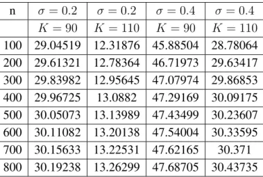
Table 1: Prices of the American lookback call option n σ= 0.2 σ= 0.2 σ= 0.4 σ = 0.4 K = 90 K = 110 K = 90 K = 110 100 29.04519 12.31876 45.88504 28.78064 200 29.61321 12.78364 46.71973 29.63417 300 29.83982 12.95645 47.07974 29.86853 400 29.96725 13.0882 47.29169 30.09175 500 30.05073 13.13989 47.43499 30.23607 600 30.11082 13.20138 47.54004 30.33595 700 30.15633 13.22531 47.62165 30.371 800 30.19238 13.26299 47.68705 30.43735
3.4
Numerical examples
For pricing American lookback call option with singular points method we made the Matlab program (see Appendix). We use the following initial values: the initial value of the stock price is S0 = 100, the maturity T = 1, the interest rate
r = 0.1. We consider two choices for the volatility: σ = 0.2, σ = 0.4and two choices for the strike price: K = 90andK = 110. We consider different time steps n = 100; 200; 300; 400; 500; 600; 700; 800. The numerical results are in table 1.
References
[1] Babbs, S. (2009): Binomial Valuation of Lookback options. J.Econ. Dynam. Control 24, 1499-1525.
[2] Desmond, J. (1996)An Introduction to Financial Option Valuation .Cambridge University Press.
[3] Ralph, K., & Elke, K. (2001)Option Pricing and Portfolio Optimization. Amer-ican Mathematical Society.
[4] Barraquand, J.& Pudet., T (1996) Pricing of American Path dependent claims.
Mathematical Finance,6, 17–51.2
[5] Buchanan, J.R (2012) An Undergraduate Introduction to Financial Mathemat-ics.World Scientific Publishing Co.Pte.Ltd.
[6] Cox, J.& Ross., S.A (1979) Option Pricing: A simplified approach. Journal of Financial Economics,7, 229–264.
[7] Hull, J.& White., A. (1993) Efficient Procedures for Valuing European and American Path-dependent Options. Journal of Derivatives,1, 21–31.
[8] Jiang, L.& Dai., M. (2005) : Convergence of binomial tree methods for Eu-ropean/American Path dependent Options. SIM Journal of numerical analysis , 42-3, 1094–1109.
[9] Stanley, R.P (1997) Introduction to Financial Mathematics: Mathematical Models and Computation.Oxford Financial Press.
[10] Wilmott, P.& Dewynne., I.& Howison., S. (1993) Option pricing: Discrete Time Models.Blackwell Publishing Ltd.
A
Matlab code for singular point method
clc clear for s1=1:2 sigma=0.2*s1; for s2=1:2 K=90+20*(s2-1); for nn=1:8%% Parameters of the binomial model n=100*nn; s0=100; r=0.1; T=1; q=0.03; delta_t=T/n; u=exp(sigma*sqrt(delta_t)); d=1/u; p=(exp(r*delta_t)-d)/(u-d); P(1:n+1,1:100)=0; M(1:n+1,1:100)=0; P_new(1:n+1,1:100)=0; M_new(1:n+1,1:100)=0;
%% Singular points at maturity (n) for j=0:n j1=j+1; S(j1)=s0*u^(2*j-n); V(j1)=max(S(j1)-K,0); Mmin(j1)=max(s0,S(j1)); Mmax(j1)=s0*u^j; if j==0 || j==n M(j1,1)=Mmin(j1); P(j1,1)=max(Mmin(j1)-K,0); L(j1)=1; else
if K>Mmin(j1) && K<Mmax(j1) M(j1,1)=Mmin(j1);
P(j1,1)=0; M(j1,2)=K; P(j1,2)=0; M(j1,3)=Mmax(j1); P(j1,3)=Mmin(j1)-K; L(j1)=3; else M(j1,1)=Mmin(j1); P(j1,1)=max(Mmin(j1)-K,0); M(j1,2)=Mmax(j1); P(j1,2)=max(Mmax(j1)-K,0); L(j1)=2; end end end %% Singular points j=0,1,...,n-1 for k=n-1:-1:0 for j=0:1:k j1=j+1; S(j1)=s0*u^(2*j-k); Mmin(j1)=max(s0,S(j1)); Mmax(j1)=s0*u^j;
%% Singular points in case of j=0 or j=k if j==0 || j==k M_new(j1,1)=Mmin(j1); if j==0 P_new(j1,1)=exp(-r*delta_t)* (p*P(j1,1)+(1-p)*P(j1+1,1)); else P_new(j1,1)=exp(-r*delta_t)* (p*P(j1,1)+(1-p)*P(j1+1,L(j1+1))); end P_new(j1,1)=max(P_new(j1,1),Mmin(j1)-K); L_new(j1)=1; else
%% singular points in case 1<=j<=k-1
vcmax(j1)=Vc(Mmax(j1),P,M,L,j1,r,delta_t,p,u); if vcmin(j1)<=Mmin(j1)-K M_new(j1,1)=Mmin(j1); P_new(j1,1)=Mmin(j1)-K; M_new(j1,2)=Mmax(j1); P_new(j1,2)=Mmax(j1)-K; L_new(j1)=2; else M_new(j1,1)=Mmin(j1); P_new(j1,1)=max(vcmin(j1),Mmin(j1)-K); L_new(j1)=1;
if K>Mmin(j1) && K <Mmax(j1) M_new(j1,2)=K; vck(j1)=Vc(K,P,M,L,j1,r,delta_t,p,u); P_new(j1,2)=max(vck(j1),K-K); L_new(j1)=L_new(j1)+1; end for jt=1:L(j1+1) if M(j1+1,jt)>K && M(j1+1,jt)<Mmax(j1) vck(j1)=Vc(M(j1+1,jt),P,M,L,j1,r,delta_t,p,u); if vcmax(j1)>=Mmax(j1)-K && vck(j1)<=M(j1+1,jt)-K else M_new(j1,L_new(j1)+1)=M(j1+1,jt); P_new(j1,L_new(j1)+1)=vck(j1); L_new(j1)=L_new(j1)+1; end end end M_new(j1,L_new(j1)+1)=Mmax(j1); P_new(j1,L_new(j1)+1)=max(vcmax(j1),Mmax(j1)-K); L_new(j1)=L_new(j1)+1; end end end for j=0:1:k
j1=j+1; L(j1)=L_new(j1); for k1=1:L(j1) M(j1,k1)=M_new(j1,k1); P(j1,k1)=P_new(j1,k1); end end end hh=2*(s2-1)+s1; Price(nn,hh)=P(1,1); end end end
function VC = Vc(M1,P,M,L,j1,r,delta_t,p,u) if L(j1+1)==1 V2=P(j1+1,1); else if M1<M(j1+1,1) %%&& M1>=M(j1+1,1)/u V2=P(j1+1,1); else for jt=1:L(j1+1)-1 if M1<=M(j1+1,jt+1) && M1>=M(j1+1,jt) V2=P(j1+1,jt)+(M1-M(j1+1,jt))*(P(j1+1,jt+1)-P(j1+1,jt))/ (M(j1+1,jt+1)-M(j1+1,jt)); end end end end if L(j1)==1 V1=P(j1,1); else for jt=1:L(j1)-1 if M1<=M(j1,jt+1) && M1>=M(j1,jt) V1=P(j1,jt)+(M1-M(j1,jt))*(P(j1,jt+1)-P(j1,jt))/ (M(j1,jt+1)-M(j1,jt)); end end end VC=exp(-r*delta_t)*(p*V2+(1-p)*V1);
*Non-exclusive licence to reproduce thesis and make thesis public I,Samuel Amankwaa (date of birth: 07.07.1983),
1. herewith grant the University of Tartu a free permit (non-exclusive licence) to:
(a) reproduce, for the purpose of preservation and making available to the public, including for addition to the DSpace digital archives until expiry of the term of validity of the copyright, and
(b) make available to the public via the web environment of the University of Tartu, including via the DSpace digital archives until expiry of the term of validity of the copyright,"Singular points binomial method for pricing American fixed lookback options” supervised by Toomas Raus, 2. I am aware of the fact that the author retains these rights.
3. I certify that granting the non-exclusive licence does not infringe the intellec-tual property rights or rights arising from the Personal Data Protection Act.