This is a repository copy of
A probabilistic patient scheduling model for reducing the
number of no-shows
.
White Rose Research Online URL for this paper:
http://eprints.whiterose.ac.uk/151553/
Version: Accepted Version
Article:
Ruiz-Hernández, D., García-Heredia, D., Delgado-Gómez, D. et al. (1 more author) (2019)
A probabilistic patient scheduling model for reducing the number of no-shows. Journal of
the Operational Research Society. ISSN 0160-5682
https://doi.org/10.1080/01605682.2019.1658552
This is an Accepted Manuscript of an article published by Taylor & Francis in Journal of the
Operational Research Society on 10th September 2019, available online:
http://www.tandfonline.com/10.1080/01605682.2019.1658552
Reuse
Items deposited in White Rose Research Online are protected by copyright, with all rights reserved unless indicated otherwise. They may be downloaded and/or printed for private study, or other acts as permitted by national copyright laws. The publisher or other rights holders may allow further reproduction and re-use of the full text version. This is indicated by the licence information on the White Rose Research Online record for the item.
Takedown
If you consider content in White Rose Research Online to be in breach of UK law, please notify us by
A probabilistic patient scheduling model for reducing the
1number of no-shows
2Diego Ruiz-Hern´andeza David Garc´ıa-Herediab David Delgado-G´omezb
3
Enrique Baca-Garc´ıac
aSheffield University Management School, Sheffield, UK
bDepartment of Statistics, Universidad Carlos III de Madrid, Legan´es, Spain cDepartment of Psychiatry, Fundaci´on Jim´enez D´ıaz, Madrid, Spain 4
Abstract 5
Patients who do not attend their appointments, or “no-shows”, cause the
under-6
utilisation of the health centres’ resources and increase the average waiting time for
7
accessing specialty health care services. Although this problem has been addressed in
8
different appointment scheduling models, behavioural issues associated to the patient’s
9
socio-demographic and economic characteristics and/or his or her diagnosis, have not
10
been widely included in scheduling optimisation models. In this article, we propose an
11
integer linear programming model thattakes into account such behavioural issues in
or-12
der to reduce impact of no-shows in medical services. To achieve this goal, the objective
13
function maximises the health centre’s expected revenue by using show-up probabilities
14
estimated for each combination of patient and appointment slot. These behaviour-based
15
probabilities are obtained using both the individual’s personal and clinical characteristics
16
and his or her attendance history. In addition, the model takes into account the
require-17
ments imposed by both the health centre’s management and the health authorities (e.g.
18
distinguishing between first visits and follow-ups, among others). An extension of the
19
model allows overbooking in some appointment slots. Experimental results show that
20
the proposed model is capable of reducing the waiting list length by 13% and to attain
21
an increase of about 5% in revenue when comparing to a basic model that assigns each
patient to the first available slot. It was also observed that when overbooking was allowed
23
in one to three slots per day, the waiting list was reduced between 30% and 62%; and
24
the revenue increased by 7% to 13%.
25
Keywords: appointment scheduling; no-shows; overbooking; healthcare; behavioural
26
OR
27
1
Introduction
28
Over the past decades, there has been a considerable increase on health care expenditures
29
worldwide. For instance, in the United States, the percentage of the GDP spent on health has
30
increased from the 12.51% in 2000 to the 16.84% in 2015 (World Bank, 2018). A not negligible
31
part of this expense is caused by the patients, commonly referred to as no-shows, who do not
32
show-up for their appointments. For example, Moore et al. (2001) concluded that “over the
33
course of a year, total revenue shortfalls [due to no-shows] could range from 3% to 14% of
34
total clinic income”; likewise, Berg et al. (2013) estimated daily losses of about 16.5% of the
35
revenue for a no-show rate of about 18%. In overall, McKee (2014) estimates that no-shows
36
cost the American healthcare industry around 150 billion dollars per year. No-shows have
37
also an important negative effect on the efficiency of health systems, causing under-utilisation
38
of resources, long waiting lists and decreased revenue. The volume of no-shows depends on
39
elements as disparate as the region, the patient’s socio-demographic characteristics, clinical
40
diagnosis and prior no-show history, as well as the specialty and the type of service provided,
41
among others (Dantas et al., 2018). In their literature review, Kheirkhah et al. (2015) refer
42
reported no-show rates ranging from 3 to 80 percent. Along the same line, Moore et al.
43
(2001) observed that no-shows and cancellations represent about 32.2% of scheduled time at
44
a family planning residence clinic.
45
In order to reduce these figures, health centres utilise two alternative approaches. On
46
one hand, the so-called active approaches include reminders and sanctions. The success of
47
these methods is uncertain, with some research reports showing a drastic reduction in the
48
percentage of no-shows after these measures are implemented (Molfenter, 2013), while others
49
find no differences or, at most, a modest reduction (Hixon et al., 1999; Satiani et al., 2009).
This difference can be explained by the fact that the effectiveness of these methods may
51
depend on the characteristics of the target population (Hashim et al., 2001). On the other
52
hand, the so-called passive approaches aim at improving the current appointment system
53
of the health centre by means of more sophisticated (and efficient) appointment assignment
54
policies, instead of the most frequent practice of assigning the patient to the first available
55
slot.
56
Optimising patient appointment systems has been an active subject of research over the
57
last few decades (Cayirli and Veral, 2003; Gupta and Denton, 2008; Ahmadi-Javid et al.,
58
2017). The patient allocation systems that have been proposed in the scientific literature
59
present several differences, which are mainly consequence of the specific characteristics of
60
the health centre and the type of service provided. For example, some centres establish that
61
patients must receive their appointment at the time when this is requested, while in other
62
cases appointments are scheduled at the end of certain period (the patient is notified later
63
on by physical or electronic means). These two approaches are usually named as online and
64
offline, respectively (Zacharias and Pinedo, 2014). Although online systems are the most
65
frequently used, the rapid development of electronic appointment systems has caused an
66
increase in the relevance of offline systems (Ahmadi-Javid et al., 2017). Another difference is
67
whether the scheduling system admits overbookings or not, although most of the proposed
68
systems include overbooking in their models (LaGanga and Lawrence, 2007; Chakraborty
69
et al., 2010; Kim and Giachetti, 2006). A more detailed description of the different types
70
of appointment systems can be found in the recent review conducted (Ahmadi-Javid et al.,
71
2017).
72
Notwithstanding there is evidence that the probability that a patient will show-up to an
73
appointment is closely related to his or her socio-demographic characteristics and condition
74
(Dantas et al., 2018), traditional appointment scheduling models for medical services are
75
usually based on the availability of slots, practitioner’s timetables, and visit times, among
76
other characteritics of the service provided. Only seldom, the proposed models take into
77
consideration the probability that a patient will attend an appointment in a given time
78
window. Moreover, those models tend to allocate probabilities based in generic data without
taking into account characteristics and behavioural traits specific to each patient.
80
This article constitutes an effort for bringing the field of behavioural operational
re-81
search to the area of patient schedulling, by proposing an appointment planning method
82
that takes into account each individual’s probabilities of no-show (estimated from their
socio-83
demographic characteristics, diagnose and attendance history) for each specific combination
84
of time-slot and patient. In doing so, our work seeks to fill a gap existing in the application of
85
OR in healthcare (comprehensive reviews include those by Brailsford et al. (2009) and Hulshof
86
et al. (2012)) through the development of behaviourally informed approaches (H¨am¨al¨ainen
87
et al., 2013), that aim at improving the provision of medical services by including associated
88
patient’s behaviour in the modelling process.
89
In this article, an integer linear programming (ILP) model is developed for optimising the
90
offline assignment of medical appointments in a speciality service of a public health centre.
91
The system aims at minimising the number of no-shows, and indirectly the waiting list length.
92
This is attained by means of an objective function that maximising the expected revenue of
93
the health centre. The model is designed as a single server system accounting for the fact
94
that, in general, each practitioner has his own list of patients. Finally, as the health centre
95
may be required by law to serve a fixed proportion of new patients every week, the model
96
includes the possibility of reserving a percentage of slots for first-visits.
97
Under certain conditions, in order to reduce the large number of practitioners’ idle periods
98
caused by no-shows, a health centre may consider the possibility of introducing overbooking
99
in some slots. This may also have a positive impact on the length of the waiting list (mainly in
100
centres with large incidence of no-shows). For those cases, we propose a mixed integer linear
101
programming (MILP) formulation that extends the initial model by allowing overbooking in
102
a limited (pre-defined) number of slots.
103
Before introducing the mathematical formulation of the system, in Section 2, we provide a
104
brief description of some related approaches available in the literature. In section 3 we present
105
the proposed mathematical model. In Section 4 we conduct a simulation experiment in order
106
to test our model’s performance. We conclude this article in Section 5 with a discussion of
107
the results and pointing out future lines of research.
2
Related literature
109
As mentioned above, several models have been proposed for improving patients’ access to
110
health care. The differences in these models are mainly consequence of the heterogeneity
111
of the requirements imposed by the health centres (e.g. online or offline scheduling, single
112
or multiple servers or if no-shows should be taken into account) and the goals pursued (e.g.
113
maximise the revenue or reduce the length of the waiting list). In this section we focus
114
our discussion on the analysis of those models most closely related to our work: first, we
115
discuss the offline mathematical programming models (either ILP or MILP) proposed for
116
single server systems; later, we present a review of some of the most relevant works that take
117
into account the presence of no-shows from a probabilistic perspective.
118
Conforti, Guerreiro and Guido developed various ILP models that maximise the number
119
of patients –weighted by the severity of their illnesses- scheduled for starting a radiotherapy
120
treatment (Conforti et al., 2008, 2011). Their models assign each patient to several time slots
121
during a given number of weeks so that the treatment can be conducted without interruptions.
122
This assignment is conducted taking into account the constraints generated by patients that
123
have already started the treatment. Zhu et al. developed a similar model for scheduling the
124
access to a Magnetic Resonance Imaging scanner (Zhu et al., 2012). Their model assigns
125
the patients to the required time slots in a two-week schedule so the number of allocated
126
patients, weighted by their priorities, is maximised. Their model takes into account patients’
127
time availability. Wang and Fung developed a model aiming at maximising profit, measured
128
as the revenue earned from the attended patients minus the cost incurred from patients’
129
rejection (Wang and Fung, 2014). The revenue was dependent on the patients’ preferences
130
for appointment time and practitioner. Additionally, a constraint was included for limiting
131
the degree of discrepancy between the time allocated and the patient’s preferences. More
132
recently, Wiesche, Schacht and Werner proposed a MILP model that seeks to minimise the
133
number of assigned appointments, penalising the number of patient shifted from morning to
134
afternoon sessions (Wiesche et al., 2017). This allowed the authors, in one hand, to increase
135
the time availability for attending walk-ins, and to balance the physicians’ workload, on the
136
other.
However, the models discussed above do not consider the existence of no-shows. In this
138
regard, Savelbersbergh and Smilowitcz developed an ILP model whose objective function
139
aimed at maximising the health condition of the population in a mobile asthma management
140
program (Savelsbergh and Smilowitz, 2016). The health condition was measured by the
141
likelihood that a patient’s disease was controlled, which was strongly related to the probability
142
that the patient showed-up to his appointment. The authors defined no-show probabilities
143
for six different categories of patients depending on their preferences (strong or weak) for
144
three different time windows (AM, noon, or PM) and 8 time slots in each time window. To
145
our knowledge, this is the only offline ILP model that, although implicitly, takes into account
146
the existence of no-shows.
147
Regarding the works that include no-show information from a probabilistic point of view,
148
we find that most of them are developed from an on-line perspective and formulated as
149
Stochastic Programming or Markov Decision Problems (Ahmadi-Javid et al., 2017). For
ex-150
ample, Muthuraman and Lawley developed a stochastic overbooking model that considered
151
each patient’s no-show probability (Muthuraman and Lawley, 2008). The objective function
152
aimed at maximising the revenue penalised by an overbooking cost, represented by the
pa-153
tient’s waiting time and staff’s overtime. This model was later tested by Daggy et al. on
154
real data where the no-show probabilities were estimated applying a logistic regression to a
155
dataset obtained from a Veterans Affairs medical centre (Daggy et al., 2010). In a different
156
work, Glowacka, Henry and May estimated the probabilities that a patient will show-up to
157
his or her appointment by means of an association rule mining technique (Glowacka et al.,
158
2009). They used these probabilities to derive three manageable sets of rules for patient
159
scheduling. Recently, Samorani and Laganga have proposed an online scheduling model that
160
admits overbooking, and whose objective function aims at maximising the revenue penalised
161
by the patients’ waiting time and overtime cost. Instead of a probabilistic classifier, they use
162
a binary one to maintain their problem computational tractable (Samorani and LaGanga,
163
2015).
164
The model proposed in this article extends the available literature in appointment
schedul-165
ing for health centres in the following directions. First, unlike most of the mathematical
programming-based research, our model takes into consideration the likelihood that a
pa-167
tient will not show-up to his or her appointment. Secondly, our formulation adopts an off-line
168
approach that uses differentiated show-up profiles for each patient. These show-up profiles,
169
that provide a specific show-up probability for each available slot, are obtained using
socio-170
demographic and clinical characteristics of the patient. This is an important difference with
171
respect to other available probabilistic work, which uses predominantly on-line approaches
172
and/or where the no-show probabilities are either categorised (Savelsbergh and Smilowitz,
173
2016) or binarised (Samorani and LaGanga, 2015). A third characteristic is that, unlike other
174
works that consider first visits and follow-ups as homogeneous groups or, plainly, ignore the
175
first visit group (Daggy et al., 2010), our formulation distinguishes among them, allowing
176
the model, apart from satisfying a legal requirement, to exploit the different characteristics
177
of these groups. Finally, our model allocates priorities to the patients depending on the time
178
they have been in the waiting list.
179
3
The Probabilistic Patient Scheduling Problem
180
In this section, we introduce a probabilistic scheduling model for reducing no-shows in
spe-181
cialty health centres that takes into consideration patient-specific probabilities of showing
182
at each given day/time slot. The objective is maximising the centre’s expected revenue by
183
means of a reduction in the number of no-shows. The model distinguishes between two types
184
of patients (first visits and follow-ups) and, by using a priority value associated to each
pa-185
tient, takes into account the time that the patient has remained in the waiting list. It also
186
takes into account a Spanish legal constraint regarding the proportion of first visits that must
187
be scheduled every week.
188
The following notation will be used in the mathematical formulation of the model.
189
Sets
190
I, days of the week;
191
J, time slots available in any given day;
192
K, set of patients to be scheduled for appointment during the reference week.
Parameters
194
q, proportion of the number of available slots that must be allocated to first visits;
195
dk, binary parameter indicating if patientk∈ K has high (dk = 0) or low (dk = 1) priority 196
during the reference week;
197
Zk, binary parameter indicating if patient k ∈ K is a first visit (Zk = 1) or a follow-up 198
(Zk = 0); 199
Pi,j,k, probability that patient k ∈ K will show-up to an appointment in slot {i, j}, for all 200
i∈ I and j∈ J;
201
wz, revenue obtained either from a first visit (z= 1), or a follow-up (z= 0). 202
Variables
203
Xi,j,k, binary variable taking value 1 if patient k∈ K is assigned to slot {i, j}, for all i∈ I 204
and j∈ J.
205
XT
k, binary variable taking value 0 if patient k ∈ K is assigned a slot in the current week 206
and 1 if the patient is referred back to the waiting list.
207
With this notation, and taking into account that the operator ⌈·⌉ rounds a real number
208
to its upper integer value, the model is formulated as follows:
209 max X i∈I X j∈J X k∈K Xi,j,kPi,j,k(Zkw1+ (1−Zk)w0) (1) s.t. X k∈K Xi,j,k ≤1, ∀i∈ I, j∈ J (2) X i∈I X j∈J Xi,j,k+XkT = 1, ∀k∈ K (3) X i∈I X j∈J X k∈K Xi,j,kZk≥min X k∈K Zk,⌈q|I||J|⌉ , (4)
X i∈I X j∈J X k∈K Xi,j,k(1−dk)≥min n X k∈K (1−dk), (5) |I||J| −min X k∈K Zk,⌈q|I||J|⌉ o , Xi,j,k, XkT ∈ {0,1}, ∀i∈ I, j∈ J, k∈ K. (6)
The objective function maximises the cllinic’s expected revenue. Notice that whenw0 = 210
w1 = w the objective function maximises the expected showing-up rate; otherwise, the 211
objective maximises the expected weighted showing-up rate. Constraints (2) guarantee that
212
only one patient is assigned to each slot. Constraints (3) make sure that if a patient is not
213
allocated in the current week, he or she is returned to the waiting list. As we are working
214
with binary variables, constraints (3) also ensure that each patient is not allocated in more
215
than one slot. Constraint (4) forces to reserve a number of slots for the first time visits.
216
Constraint (5) guarantees that low priority patients will not be allocated to a slot as long as
217
there are high priority patients unallocated.
218
Model with overbooking
219
As mentioned in the Introduction, there may be cases in which performing overbooking is
220
considered convenient. For these situations, the baseline model is extended for allowing the
221
possibility of assigning two patients to the same slot, provided that the sum of their
showing-222
up probabilities is less than certain predetermined value. This is attained by introducing an
223
overbooking penalty in the objective function and a number of associated constraints. The
224
following additional notation is used in the extended model:
225
Parameters
226
Cov, positive parameter representing the overbooking penalty; 227
M, constant satisfying M >max{w0, w1}; 228
Gi,j, binary parameter taking value 1 if overbooking is allowed in slot {i, j}, for all i ∈ I 229
and j∈ J;
πi,j, parameter imposing a bound on the sum of the showing-up probabilities for any pair of 231
patients simultaneously booked in slot {i, j},for alli∈ I and j∈ J 1 .
232
Variables
233
Yi,j, binary variable taking value 1 if overbooking has been used in slot {i, j}, for all i∈ I 234
and j∈ J;
235
Oi,j, binary variable taking value 1 if at least one patient has been booked in slot{i, j}, for 236
all i∈ I and j∈ J.
237
The model with overbooking is then given by:
max X i∈I X j∈J X k∈K
Xi,j,kPi,j,k(Zkw1+ (1−Zk)w0)−CovYi,j+M Oi,j (7)
s.t. Constraints (3)-(5), and Yi,j ≤Gi,j, ∀i∈ I, j∈ J (8) X k∈K Xi,j,k ≤1 +Yi,j, ∀i∈ I, j∈ J (9) X k∈K
Xi,j,kPi,j,k ≤πi,j, ∀i∈ I, j∈ J (10)
Oi,j ≤
X
k∈K
Xi,j,k, ∀i∈ I, j∈ J (11)
Xi,j,k, XkT, Yi,j, Oi,j∈ {0,1}, ∀i∈ I, j∈ J, k ∈ K (12)
The CovYi,j term in the extended objective function, equation (7), represents a penalty 238
incurred when overbooking is used in slot {i, j}. Please notice that this term attains the
239
largest possible reduction in the practitioners’ idle times by allocating the same slot (if
240
overbooking is admissible) to the pair of patients with highest sum of show-up probabilities.
241
This is guaranteed by the fact that the larger the weighted sum of show-up probabilities,
242
the larger the profit after discounting the overbooking cost for any given slot. Notice also
243
that ifCov <{w0, w1} ×mini,j,k{Pi,j,k}, the model will always use overbooking when|K|> 244
1Notice that the probability of both patients showing-up is given byPi,j,k·Pi,j,k′, which attains a maximum
atPi,j,k=Pi,j,k′=
πij
|I||J |, i.e. whenever the number of patients in the waiting list is larger than the number of
245
available slots. Likewise, if Cov >max{w0, w1} ×maxi,j,k{Pi,j,k}, the model will never use 246
overbooking.
247
Regarding the associated constraints, equations (8) define the slots where overbooking
248
is allowed. Equations (9) limit the number of overbooked patients in a given slot to two,
249
provided that overbooking is allowed. Finally, in order to control for the maximal probability
250
of overcrowding (the case where two overbooked patients show-up for the same appointment),
251
the sum of showing-up probabilities in an overbooked slot is bounded by parameter πij in 252
constraints (10).
253
TermM Oij in equation (7), together with constraints (11) and the fact that by definition 254
M >max{w0, w1}, ensures that the model does not consider overbooking unless all slots are 255
used.
256
Additionally, our model presents the following two properties, which will be used in the
257
computational implementation of the model for speeding up the execution:
258
Proposition 3.1. In the model with overbooking, theOi,j variables always take integer values 259
when they are relaxed to 0≤Oi,j ≤1 for alli∈ I, j∈ J. 260
Proof. Let Oij be a continuous variable defined in the interval [0,1] for all i∈ I, j ∈ J. If 261
P
k∈KXi,j,k = 0, from constraint (11) it immediately follows thatOij = 0. Alternatively, if 262
P
k∈KXi,j,k > 0 and given that the Xijk are binary variables, then Oij can take any value 263
in the interval [0,1]. However, given that M Oij appears with positive sign in the objective 264
function of the maximisation problem, it follows thatOij = 1. 265
Proposition 3.2. In the model with overbooking, theYi,j variables always take integer values 266
when they are relaxed to 0≤Yi,j ≤1 for alli∈ I, j∈ J. 267
Proof. LetYi,j be a continuous variable defined in the interval [0,1] for alli∈ I, j∈ J. We 268
consider two possible scenarios:
269
1. |K| ≤ |I||J|: From the objective function if follows directly that Yij = 0 for all i ∈ 270
I, j ∈ J. Double booking any slot, when a number of slots remains unallocated, will
271
imply unnecessarily incurring a penalty of Cov. 272
2. |K| > |I||J|: Consider any given slot {i, j}. If overbooking is not allowed, Gi,j = 0, 273
constraints (8) guarantee thatYij = 0. 274
Assume now that overbooking is allowed and conducted at some slot{i, j}, i.e. Gij = 1 275
and P
k∈KXi,j,k = 2. Let Yi,j = δ with 0 < δ < 1, satisfying constraints (8). From 276
constraints (9) it follows that P
k∈KXi,j,k ≤ 1 +δ, and given that Xi,j,k ∈ {0,1} we 277
conclude that P
k∈KXi,j,k ≤ 1, which is a contradiction. Therefore, if slot {i, j} is 278
overbooked, then necessarilyYij = 1. 279
Finally, assume that overbooking is allowed but not conducted at some slot{i, j}, i.e.
280
Gij = 1 andPk∈KXi,j,k= 1. LetYi,j =δwith 0< δ <1, satisfying constraints (8). As 281
before, constraints (9) imply thatP
k∈KXi,j,k≤1 +δ, and given thatXi,j,k ∈ {0,1} it 282
still holds thatP
k∈KXi,j,k ≤1. Now, given that CovYij appears with negative sign in 283
the objective function of the maximisation problem, it follows thatYij = 0. Therefore, 284
if slot{i, j}is not overbooked, then immediately Yij = 0. 285
286
Comment
287
If instead of a penalty for overbooking, an expected cost for overcrowding was the driver
288
behind the overbooking decision, the corresponding term in the objective function –and the
289
associated constraints- will need to incorporate the overcrowding probability (the product
290
of the attendance probabilities of the two overbooked patients). In this case, the objective
291
function will seek to allocating the overbooked slots to the pair of patients with lowest product
292
of show-up probabilities. Consequently, with the aim of minimising the overcrowding penalty,
293
the system will still face large idle times (as the probability of none of the patients showing-up
294
will still be large). Moreover, the problem will become non-linear.
295
3.1 Scheduling Procedure
296
The scheduling procedure works as follows:
297
1. A waiting list is available with the records of the patients waiting for appointment,
298
including information about the number of weeks they have been in the list (sojourn)
and whether it is a first-time visit or not. New patients are added to the list at the
300
time the appointment request is received and their sojourn length counter is initialised
301
to zero.
302
2. The list of patients (henceforth referred to as thebuffer) to be passed each week to the
303
scheduler is built as follows:
304
(a) The system first selects the patients with largest sojourn value and assigns them
305
high priority (dk = 0). This group contains both first-visits (Zk = 1) and follow-306
ups (Zk = 0). 307
(b) Once the high priority patients have been selected, if the number of first-visits
308
in the buffer is still below the legal requirement, the system sequentially adds
309
first-visits in decreasing order of sojourn length until the requirement is satisfied
310
or no more first visits are left in the waiting list. At each iteration, all first-visits
311
in the corresponding sojourn level are included. These patients have low priority
312
(dk= 1) andZk= 1. 313
(c) Finally, if after including high priority patients and first-visits, the number of
314
patients in the buffer is smaller than the number of available slots (and there
315
are still patients in the waiting list), the system sequentially adds patients in
316
decreasing order of sojourn length until the size of the buffer is larger or equal to
317
the number of available slots (or the waiting list is empty). At each iteration, all
318
patients in the corresponding sojourn level are included. These patients have low
319
priority (dk= 1). 320
3. After this selection has been conducted, the system passes the list of candidates to
321
the scheduler for solving the Probabilistic Patient Scheduling Problem with or without
322
overbooking. Once the schedule has been obtained, the patients who did not receive
323
an appointment are sent back to the waiting list with their original sojourn value.
324
Regarding the overbooking policy, whenever two patients show up for the same
appoint-325
ment, subsequent appointments are delayed until either a no-show happens and the last
delayed patient takes that slot, in which case the original schedule is reestablished, or the
327
day finishes and the practitioner does over-time until the list is cleared. Please notice that the
328
over-time impact of this policy will be limited as long as the number of slots where overtime
329
is admissible does not exceed a reasonable limit (e.g. no more than 2 or 3 slots).
330
4
Numerical Experiments
331
In order to evaluate the performance of our model, an experiment that reproduces the routine
332
of a psychiatry department in a Spanish health centre was designed. In order to estimate the
333
probabilities that the patients would show-up for their appointments, a database containing
334
information from 47,118 visits to this department was used. In addition to the variable
335
indicating whether the patient attended the appointment or not, this database contains
336
several variables that have been frequently used to characterise non-shows. These variables
337
were age (Alaeddini et al., 2011; Kopach et al., 2007), sex (Alaeddini et al., 2011), week day
338
and time of the appointment (Glowacka et al., 2009; Daggy et al., 2010), lead time (time in
339
queue) in weeks (Daggy et al., 2010), practitioner ID, appointment type (first visit or
follow-340
up) (Kopach et al., 2007), number of previous appointments (Kopach et al., 2007; Daggy
341
et al., 2010), and percentage of no-shows in previous appointments (Kopach et al., 2007;
342
Daggy et al., 2010). The probabilities of show-up were obtained using a decision tree (Norris
343
et al., 2014) classifier. The use of the database allowed us to obtain specific and differentiated
344
attendance probabilities for each available appointment slot, provided the patient’s profile.
345
The simulation is conducted as follows:
346
1. At the beginning of each week, we generate the set of patients who call for a new
347
appointment. To do this, a random number is generated according to a discrete
uni-348
form variable whose parameters are provided below. This number is used for randomly
349
selecting a number of patients from our database. By doing this, we respect the
pro-350
portion of first visits/follow-ups as well as the distribution of the variables representing
351
the patients’ characteristics. The selected patients are added-up at the end of the
wait-352
ing list. Each patient in the waiting list has assigned a sojourn value representing the
number of weeks that he or she has remained in the list. New arrivals are all assigned
354
a sojourn value equal to zero.
355
2. The list of patients to be passed each week to the scheduling model is built as described
356
in item 2 of Section 3.1.
357
3. After this selection has been performed, the Probabilistic Patient Scheduling
Prob-358
lem is solved using the generated data2
. Once the model makes the assignment, the
359
parameters of the system are updated for the following week as follows:
360
For each appointment we randomly determine whether the patient will show-up or not
361
depending on the patient’s estimated attendance probability given the allocated slot. If
362
the patient shows-up to the appointment, the health centre obtains the corresponding
363
income and the patient is removed from the system. Otherwise, the patient is either
364
returned to the waiting list according to a predetermined probability, or eliminated
365
from the system. If returned, the patient is put at the end of the list with sojourn
366
value 0. This way, the experiment mimics the situation in which the patient that did
367
not attend an appointment asks for a new one.
368
Patients who did not receive an appointment are sent back to the waiting list with their
369
initial sojourn time.
370
4. At the end of each scheduling stage, the sojourn values of all patients in the waiting
371
list are increased by one.
372
4.1 Simulation framework
373
As we mentioned, our experiment reproduces the functioning of a psychiatry department
374
week by week during one year (52 weeks). In this centre, the doctor does consultation from
375
8:30 to 15:30 from Monday to Friday and each consultation lasts 30 minutes. Therefore,
376
if overbooking is not considered, the doctor would attend a maximum of 70 patients. Of
377
those, at least 30% are first visits to comply with the regulatory requirements. For each first
378
visit the centre receives 70 euros and for each revision 50 euros. At the beginning of the
379
simulation, it is assumed that there is a 7-week waiting list to access to the medical services.
380
For each of the simulated weeks, the following operations are performed:
381
The weekly number of new requested appointments in the simulation follows a uniform
382
[51,69] distribution. This choice, together with an estimated no-show rate of 24% and the
383
60% of no-shows who are referred back to the waiting list, returns an expected number of
384
appointment requests of 68.64 per week. These figures guarantee that the weekly number
385
of patients asking for a new appointment is always close to the 70 slots available for each
386
practitioner.
387
Using this scenario, we test the following scheduling approaches:
388
1. The probabilistic scheduling model without overbooking.
389
2. The extended model with overbooking in three different situations: allowing
overbook-390
ing just at 12:00 each day, allowing overbooking at 9:00 and at 12:00; and allowing
391
overbooking at 9:00, at 10:00 and at 12:00. The reason why we chose these hours is
392
because, in our database, they are the time-slots with the greatest number of no-shows.
393
From hereafter, they will be referred as one, two and three rows of overbooking,
re-394
spectively. In all of them, the parameter that limits the maximum expected number of
395
patients πi,j is set to 1.5. Later, we will perform a sensitivity analysis to analyse the 396
influence of this parameter.
397
3. The traditional model in which each patient is assigned to the first available slot (Daggy
398
et al., 2010). We will refer this model as a FIFO system.
399
4.2 Results
400
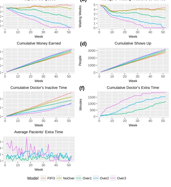
Figure 1 shows the obtained results. In these plots, the legends “NoOver”, “Over1”, “Over2”
401
and “Over3”stand for model without overbooking, and model with one, two and three rows
402
of overbooking respectively.
403
Figure 1 (a) displays the number of people in the waiting list along the different weeks.
404
It can be seen that the models which use overbooking obtain a fast reduction of the length
100 200 300 400 500 0 10 20 30 40 50 Week P eople
People in the Queue (a) 0 1 2 3 4 5 0 10 20 30 40 50 Week W aiting W eeks
Average of Waiting Weeks to be Served (b) 0 50000 100000 150000 0 10 20 30 40 50 Week Mone y
Cumulative Money Earned (c) 0 1000 2000 3000 0 10 20 30 40 50 Week P eople Cumulative Shows Up (d) 0 10000 20000 0 10 20 30 40 50 Week Min utes
Cumulative Doctor’s Inactive Time (e) 0 500 1000 1500 0 10 20 30 40 50 Week Min utes
Cumulative Doctor’s Extra Time (f) 0 2 4 6 0 10 20 30 40 50 Week Min utes
Average Pacients’ Extra Time (g)
Model FIFO NoOver Over1 Over2 Over3
of this list. It can be notice that the model which uses three rows of overbooking handles
406
to eliminate the waiting list by week 35. After this week, the queue length is stable. One
407
important result is that the proposed model that does not use overbooking (NoOver) is able
408
to maintain the queue stable while the FIFO model cannot. At the end of the experiment,
409
in week 52, the difference on the number of patients in the waiting list of these two models
410
is 70 patients, which represents the complete schedule for a week. This result indicates that
411
by only improving the patient assignment, without considering overbooking, is possible to
412
avoid that the length of the waiting list increases.
413
Figure 1 (b) exhibits the mean time that the patients remain in the waiting list. These
414
results are similar to the previous ones: the overbooking models reduce the mean time faster
415
than the other two models, and the Over3 model stabilised around week 35. As before, the
416
NoOver model attains to stabilised and the FIFO model do not. The drastic drop-out during
417
the first weeks is consequence of the initial waiting list structure.
418
Figure 1 (c) shows the cumulative revenue. As expected, the models that have the greatest
419
incomes are the overbooking models, followed by the NoOver and the FIFO models.
420
Figure 1 (d) illustrates the cumulative number of people who show up to the appointment.
421
It can be noticed that this value is greater for the overbooking models. It is sensible to think
422
that it is consequence of the fact that these models assign more patients, but it is also
423
because these patients are optimally scheduled. This fact can also be appreciated in the
424
NoOver and FIFO models. Despite they have the same number of assigned patients, the
425
number of patients who show up is higher for the NoOVer model.
426
Figure 1 (e) shows the cumulative doctor’s idle time. The first interesting fact is that
427
this value is higher in the FIFO model that in the NoOver model even though doctors in
428
these models have assigned the same number of patients. It was observed that FIFO had
429
an average of 3.5 empty slots per day, while NoOver just 2.8. Regarding the overbooking
430
models, it can be observed that, at the end of the simulation, models Over2 and Over3 have
431
a similar cumulative doctor’s idle time. This is, again, consequence that after week 35, the
432
length of the waiting list for the Over3 model is minimal.
433
Figure 1 (f) displays doctor’s overtime in which the effect of adding an extra row to the
overbooking model can be appreciated. It is important to differentiate the curves before and
435
after week 35 because, for the Over3 model, the waiting list is practically zero after this week
436
as it was commented before. Therefore, after week 35, doctor barely suffer from over time in
437
this model.
438
Figure 1 (g) represents the average time that each patient waited in the health centre to
439
be attended. It can be observed that for the Over3 model, the patients have to wait between
440
2 and 6 minutes, which is a 6% and 20% of the time of each slot.
441
442
Next, a sensibility analysis is conducted in order to assess the effect of parameter π 443
in the model’s performance. To this end, the previous experiment is repeated for values
444
{1.1,1.3,1.5,1.7}of this parameter. Table 1 shows the obtained results.
445
Number in Waiting Revenue Average Average Average doctors’ Average patients’
queue weeks (e) show-ups (%) empty slots weekly overtime (min) extra waiting time (min)
FIFO 542 4.29 145,330 75.19 3.47 0 0 NoOver 472 3.88 153,430 79.53 2.86 0 0 Over1,πi,j= 1.1 382 2.97 156,340 79.49 2.66 3.4 0.75 Over2,πi,j= 1.1 262 1.90 161,200 77.69 2.29 5.1 2.35 Over3,πi,j= 1.1 147 0.90 164,970 74.29 2.06 6.85 4.05 Over1,πi,j= 1.3 280 2.14 161,990 78.48 2.33 18.85 3.95 Over2,πi,j= 1.3 107 0.75 169,060 77.63 1.85 29.15 8 Over3,πi,j= 1.3 84 0.15 168,190 76.40 1.91 33.45 9 Over1,πi,j= 1.5 272 2.05 162,090 78.64 2.35 16.25 4.4 Over2,πi,j= 1.5 78 0 169,140 77.50 1.85 36 9.6 Over3,πi,j= 1.5 78 0 168,640 77.72 1.93 51.40 15.85 Over1,πi,j= 1.7 263 1.87 163,270 79.20 2.26 20.55 5.05 Over2,πi,j= 1.7 83 0.14 168,780 77.60 1.91 41.15 12.25 Over3,πi,j= 1.7 83 0 168,530 77.40 2 63.5 20.05
Table 1: Results of the sensitivity analysis.
Some remarks on Table 1: i) values in the first three columns correspond to week 52; ii)
values displayed in columns four and five are averages over 52 weeks; and iii) average values
447
in the last two columns are calculated over the first 35 weeks to avoid the noise caused by
448
the exhaustion of the waiting list (please see the comments around model Over3 earlier in
449
this section). Moreover, for the sake of clarity, we report the average number of empty slots
450
per day instead of doctor’s idle time.
451
We notice that the model without overcrowding (NoOver) increases the centre’s revenue
452
in 5.5% with respect to the current policy (FIFO), reducing the waiting list by 13% in
453
a year. The results show that a scheduling regime that assigns appointments taking into
454
consideration the patient’s characteristics may contribute –in the health centre under
study-455
to a reduction of about 17.5% in the number of empty slots.
456
Regarding the overbooking model, the results depend on the value assigned to parameter
457
π and the number of slots in which the overbooking is allowed (Gij = 1). If, for instance, 458
π = 1.1, it can be noticed that the impact on practitioners and patients is minimal. This is
459
due to two main reasons: i) the small probability of overcrowding (two overbooked patients
460
showing-up to the same appointment), 0.3 maximum; and ii) in the case of overcrowding, it
461
occurs early enough for a no-show in later hours to compensate for the extra time devoted
462
to attending the additional patient. For this value of π the revenue would increase in a
463
range between 7% and 13% and the waiting list would be reduced from 30% to 72%. These
464
values are consistent with the ones reported by Moore et al. (2001). We also notice that
465
allowing overbooking always improves the health centre’s revenue (with respect to the NoOver
466
case), with the maximal revenue attained when overbooking is allowed in up to two slots
467
(Over2). Moreover, allowing overbooking in two slots always reduces the number of empty
468
slots, irrespectively of the value of π.
469
Finally, regarding the value of parameter π, the best results are obtained when this
470
parameter takes values between 1.3 and 1.5. In those cases, the value of the objective
471
function increases noticeably without imposing serious penalties on the patients, with average
472
waiting times below 10 minutes for models Over1 and Over 2. These values return maximum
473
overcrowding probabilities (two overbooked patients showing-up to the same appointment)
474
of 0.42 and 0.56, respectively. This suggests that the optimal value ofπ should be such that
the overcrowding probability is close to 0.5.
476
5
Conclusions
477
In this article we address the problem of no-shows in specialty clinics. This problem imposes
478
large economic costs to the health centres –mainly due to practitioners’ idle times-, and to
479
the patients, who suffer the personal and economic impact of long waiting lists.
480
The no-shows problem is tackled in this article by proposing a scheduling strategy based
481
on a mixed-integer programming model together with a dynamic priority allocation scheme.
482
The proposed model aims at maximising the expected revenue of the health centre taking
483
into account the revenue obtained from both first visit and follow-up patients. When the
484
revenue of these two groups is the same, the objective function is equivalent to maximising the
485
expected number of show-ups. The model takes into account several constraints imposed by
486
both the law and the health centre’s policies; among them, allocating a minimum percentage
487
of the available slots to first visits, or assigning priorities based on the time the patient has
488
been in the waiting list. Our formulation can be easily adapted for considering other types of
489
priority, as jumping the queue when the severity of the patient’s condition demands it,among
490
others. The base model is extended for allowing the possibility of overbooking.
491
The maximisation of the expected number of show-ups is attained by using individualised
492
show-up probabilities which depend on the patients’ socio-demographic and personal
charac-493
teristics as well as on his or her diagnosed pathology. These probabilities are computed for
494
each day/slot combination using a decision tree classifier on a sample of nearly 50 thousand
495
visits.
496
Simulation experiments show that whereas the waiting lists size increases on time when
497
a FIFO scheduling regime is used, our base model is capable of reducing the waiting list
498
and attaining a 5% increase in revenue with respect to the FIFO regime. Experimental
499
results also suggest that a more significant reduction in the waiting list would be attained if
500
overbooking was applied. The magnitude of this reduction would naturally depend on the
501
amount of doctors’ overtime that the health centre is willing to accept. It was observed that,
502
by allowing overbooking in one time slot per day, a reduction of the waiting list of about
30% can be achieved at a minimum overtime cost. These results suggest a combined strategy
504
where limited overbooking can be initially used for obtaining a significant reduction in the
505
waiting list and, later on, switching to a regime without overbooking.
506
Our results point at two interesting research lines. The first one will aim at endogenising
507
the number and selection of the appointment slots where overbooking is allowed. Given that
508
not all the patients require the same consultation time, the second research line should extend
509
the model for taking into account the expected consultation times of the different types of
510
patient.
511
References
512
Ahmadi-Javid, A., Jalali, Z., and Klassen, K. J. (2017). Outpatient appointment systems in
513
healthcare: A review of optimization studies. European Journal of Operational Research,
514
258(1):3–34.
515
Alaeddini, A., Yang, K., Reddy, C., and Yu, S. (2011). A probabilistic model for predicting
516
the probability of no-show in hospital appointments. Health care management science,
517
14(2):146–157.
518
Berg, B. P., Murr, M., Chermak, D., Woodall, J., Pignone, M., Sandler, R. S., and Denton,
519
B. T. (2013). Estimating the cost of no-shows and evaluating the effects of mitigation
520
strategies. Medical Decision Making, 33(8):976–985.
521
Brailsford, S. C., Harper, P. R., Patel, B., and Pitt, M. (2009). An analysis of the academic
522
literature on simulation and modelling in health care. Journal of simulation, 3(3):130–140.
523
Cayirli, T. and Veral, E. (2003). Outpatient scheduling in health care: a review of literature.
524
Production and operations management, 12(4):519–549.
525
Chakraborty, S., Muthuraman, K., and Lawley, M. (2010). Sequential clinical scheduling with
526
patient no-shows and general service time distributions. IIE Transactions, 42(5):354–366.
Conforti, D., Guerriero, F., and Guido, R. (2008). Optimization models for radiotherapy
528
patient scheduling. 4OR: A Quarterly Journal of Operations Research, 6(3):263–278.
529
Conforti, D., Guerriero, F., Guido, R., and Veltri, M. (2011). An optimal decision-making
530
approach for the management of radiotherapy patients. OR Spectrum, 33(1):123–148.
531
Daggy, J., Lawley, M., Willis, D., Thayer, D., Suelzer, C., DeLaurentis, P.-C., Turkcan,
532
A., Chakraborty, S., and Sands, L. (2010). Using no-show modeling to improve clinic
533
performance. Health Informatics Journal, 16(4):246–259.
534
Dantas, L. F., Fleck, J. L., Oliveira, F. L. C., and Hamacher, S. (2018). No-shows in
535
appointment scheduling–a systematic literature review. Health Policy.
536
Glowacka, K. J., Henry, R. M., and May, J. H. (2009). A hybrid data mining/simulation
537
approach for modelling outpatient no-shows in clinic scheduling.Journal of the Operational
538
Research Society, 60(8):1056–1068.
539
Gupta, D. and Denton, B. (2008). Appointment scheduling in health care: Challenges and
540
opportunities. IIE transactions, 40(9):800–819.
541
H¨am¨al¨ainen, R. P., Luoma, J., and Saarinen, E. (2013). On the importance of behavioral
op-542
erational research: The case of understanding and communicating about dynamic systems.
543
European Journal of Operational Research, 228(3):623–634.
544
Hashim, M. J., Franks, P., and Fiscella, K. (2001). Effectiveness of telephone reminders in
545
improving rate of appointments kept at an outpatient clinic: a randomized controlled trial.
546
The Journal of the American Board of Family Practice, 14(3):193–196.
547
Hixon, A. L., Chapman, R. W., and Nuovo, J. (1999). Failure to keep clinic appointments:
548
implications for residency education and productivity. FAMILY MEDICINE-KANSAS
549
CITY-, 31:627–630.
550
Hulshof, P. J., Kortbeek, N., Boucherie, R. J., Hans, E. W., and Bakker, P. J. (2012).
551
Taxonomic classification of planning decisions in health care: a structured review of the
552
state of the art in or/ms. Health systems, 1(2):129–175.
Kheirkhah, P., Feng, Q., Travis, L. M., Tavakoli-Tabasi, S., and Sharafkhaneh, A. (2015).
554
Prevalence, predictors and economic consequences of no-shows. BMC health services
re-555
search, 16(1):13.
556
Kim, S. and Giachetti, R. E. (2006). A stochastic mathematical appointment overbooking
557
model for healthcare providers to improve profits. IEEE Transactions on systems, man,
558
and cybernetics-Part A: Systems and humans, 36(6):1211–1219.
559
Kopach, R., DeLaurentis, P.-C., Lawley, M., Muthuraman, K., Ozsen, L., Rardin, R., Wan,
560
H., Intrevado, P., Qu, X., and Willis, D. (2007). Effects of clinical characteristics on
561
successful open access scheduling. Health care management science, 10(2):111–124.
562
LaGanga, L. R. and Lawrence, S. R. (2007). Clinic overbooking to improve patient access
563
and increase provider productivity. Decision Sciences, 38(2):251–276.
564
McKee, S. (2014). Measuring the cost of patient no-shows. Power Your Practice.
565
Molfenter, T. (2013). Reducing appointment no-shows: going from theory to practice.
Sub-566
stance use & misuse, 48(9):743–749.
567
Moore, C. G., Wilson-Witherspoon, P., and Probst, J. C. (2001). Time and money: effects of
568
no-shows at a family practice residency clinic. Family Medicine-Kansas City-, 33(7):522–
569
527.
570
Muthuraman, K. and Lawley, M. (2008). A stochastic overbooking model for outpatient
571
clinical scheduling with no-shows. IIE Transactions, 40(9):820–837.
572
Norris, J. B., Kumar, C., Chand, S., Moskowitz, H., Shade, S. A., and Willis, D. R. (2014).
573
An empirical investigation into factors affecting patient cancellations and no-shows at
574
outpatient clinics. Decision Support Systems, 57:428–443.
575
Samorani, M. and LaGanga, L. R. (2015). Outpatient appointment scheduling given
in-576
dividual day-dependent no-show predictions. European Journal of Operational Research,
577
240(1):245–257.
Satiani, B., Miller, S., and Patel, D. (2009). No-show rates in the vascular laboratory: analysis
579
and possible solutions. Journal of Vascular and Interventional Radiology, 20(1):87–91.
580
Savelsbergh, M. and Smilowitz, K. (2016). Stratified patient appointment scheduling for
mo-581
bile community-based chronic disease management programs. IIE Transactions on
Health-582
care Systems Engineering, 6(2):65–78.
583
Wang, J. and Fung, Y. (2014). An integer programming formulation for outpatient scheduling
584
with patient preference. Industrial Engineering & Management Systems, 13(2):193–202.
585
Wiesche, L., Schacht, M., and Werners, B. (2017). Strategies for interday appointment
586
scheduling in primary care. Health care management science, 20(3):403–418.
587
World Bank (2018). Current health expenditure. https://data.worldbank.org.
588
Zacharias, C. and Pinedo, M. (2014). Appointment scheduling with no-shows and
overbook-589
ing. Production and Operations Management, 23(5):788–801.
590
Zhu, H., Hou, M., Wang, C., and Zhou, M. (2012). An efficient outpatient scheduling
591
approach. IEEE Transactions on Automation science and engineering, 9(4):701–709.