Boston University
OpenBU
http://open.bu.edu
BU Open Access Articles BU Open Access Articles
2017-07-31
Quantum simulation of
topologically protected states using
directionally unbiased linear-opti...
This work was made openly accessible by BU Faculty. Please
share
how this access benefits you.
Your story matters.
Version
Citation (published version): David S. Simon, Casey A. Fitzpatrick, Shuto Osawa, Alexander V.
Sergienko. 2017. "Quantum simulation of topologically protected
states using directionally unbiased linear-optical multiports."
PHYSICAL REVIEW A, Volume 96, Issue 1, pp. ? - ? (8).
https://hdl.handle.net/2144/24326
Boston University
arXiv:1708.00038v1 [quant-ph] 31 Jul 2017
Linear Optical Multiports
David S. Simon,1, 2,∗ Casey A. Fitzpatrick,2,† Shuto Osawa,2,‡ and Alexander V. Sergienko2, 3,§
1
Dept. of Physics and Astronomy, Stonehill College, 320 Washington Street, Easton, MA 02357
2
Dept. of Electrical and Computer Engineering & Photonics Center, Boston University, 8 Saint Mary’s St., Boston, MA 02215, USA
3
Dept. of Physics, Boston University, 590 Commonwealth Ave., Boston, MA 02215, USA
It is shown that quantum walks on one-dimensional arrays of special linear optical units allow the simulation of discrete-time Hamiltonian systems with distinct topological phases. In particular, a slightly modified version of the Su-Schrieffer-Heeger (SSH) system can be simulated, which exhibits states of nonzero winding number and has topologically-protected boundary states. In the large-system limit this approach uses quadratically fewer resources to carry out quantum simulations than previous linear-optical approaches and can be readily generalized to higher-dimensional systems. The basic optical units that implement this simulation consist of combinations of novel optical multiports that allow photons to reverse direction.
I. INTRODUCTION
The rapidly expanding research activity currently un-derway on quantum computing [1–4] is ultimately an out-growth of Richard Feynman’s observation that quantum systems are necessary to efficiently simulate other quan-tum systems [5–7]. The goal of quanquan-tum simulation is therefore to find simple quantum systems that can accu-rately and efficiently simulate specific properties of inter-est in more complex quantum physical entities.
The behavior of a quantum system arises from inter-ference between multiple solutions of a linear wave equa-tion. This can be seen most clearly in Feynman’s path integral formalism [8, 9], where the observable output state is a linear superposition of all allowed intermediate trajectories. In a similar manner, linear-optical systems make use of interference between light waves that arise as solutions to the linear Helmholtz equation. For sys-tems in which particle number is conserved (electrons in a solid, for example), linear optics would therefore seem to be a natural resource to exploit in order to carry out quantum simulations. In particular, photonic quantum walks [10, 11] can produce the complex interference pat-terns needed for such simulations. Because of the rel-atively feeble interactions that photons have with their surroundings, many of the complexities associated with other physical implementations of quantum simulations are greatly reduced in an optical setting. In addition, light is not only easy to produce and detect, but it can be tailor-made with a high degree of control over its fre-quency, polarization, and spatial and temporal profiles. Further, quantum effects are readily visible in optics; for example, photon pairs can be routinely produced with high degrees of entanglement [12–14].
∗e-mail: [email protected] †e-mail: [email protected] ‡e-mail: [email protected] §e-mail: [email protected]
Systems with nontrivial topological behavior arise nat-urally in the study of solids, as well as in other areas of physics. They lead to wavefunctions with nonzero Chern number or winding number, to topologically protected edge or boundary states, and to phase transitions be-tween distinct topological states (see [15–19] for reviews). Alongside theoretical work and experimental implemen-tation, quantum simulation of these behaviors has also become an active area of current research. For example, simulations have been carried out with ultracold atoms, both in free space and confined to optical lattices [20–26], as well as in photonic quantum walks [16, 27–30].
The approaches used up to now for quantum simu-lations of topologically-nontrivial physical systems have substantial limitations. For example, working with atoms requires extremely low temperatures in order to avoid de-coherence. This adds numerous complications to the ex-periments and makes this approach unlikely to be useful outside of research labs. On the other hand, analogous simulations done with optical quantum walks have their own complications. In particular, they require a set of op-tical resources (beam splitters, mirrors, etc.) that grows rapidly with the number of steps in the walk.
These factors strongly limit the ability to use the cur-rent optical approaches for practical simulations on a large scale, and so it is of interest to investigate novel schemes that may be more easily scalable. Here we present a linear-optical strategy whose resource require-ments grow at a quadratically slower rate than previous optical approaches. It is currently practical to carry out a table-top version of this procedure, and in the near fu-ture it should be plausible to implement it on much larger scales by integrating all of the required optical elements onto optical chips that can be fabricated in large num-bers and arranged into the desired configurations with high stability. In contrast to the quadratic growth in previous optical implementations, the resources required here scale only linearly with number of steps. Further-more, this scheme has the advantage that the parameters of the underlying system on which the walk occurs can
2
be readily varied to produce a variety of simulated be-haviors.
In [31] a linear-optical method was proposed for us-ing photonic quantum walks to carry out quantum sim-ulations of topologically-trivial nearest-neighbor Hamil-tonians in the context of one-dimensional discrete-time physical models. This was accomplished by means of chains of simple linear optical units. Different Hamil-tonians could be simulated by varying the arrangement of these units, or by varying their internal parameters. By going from a one-dimensional chain to two- or three-dimensional arrays, Hamiltonians exhibiting more com-plicated band gap structures can also be implemented.
In the current paper, the simple periodic lattice of [31] is replaced by a pair of two interlaced sublattices with dif-ferent parameters, leading to a substantial generalization in the types of behaviors attainable. In particular, sim-ulation of topologically non-trivial Hamiltonians become possible, with features such as nonzero winding number and topologically-protected boundary states.
The basic optical units utilized in this scheme are the directionally-unbiased optical multiports proposed in [32]. These devices can be thought of as scattering cen-ters of the type that have been discussed in the abstract context of optical graph systems [33–36]. In a graph model, an incident photon is constrained at each time step to scatter into one of a finite number of modes. One of these modes is the time-reversed version of the input mode, so it is necessary that the multiport allows the pho-ton to reverse direction and exit back out the input port. Such reversible multiports can be constructed using only linear optics and can be thought of as artificially-created optical “meta-atoms”, with lattices of them forming a type of metamaterial. In this sense, the current paper is complementary to work that seeks to produce topological behavior in dielectric metamaterials [37].
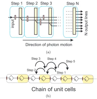
The significant reduction in resources in the current proposal compared to previous optical approaches is a direct consequence of the fact that the input ports of the unbiased multiport serve also as output ports. As a result, the flow of photons can reverse direction and traverse the same unit multiple times instead of needing additional units at each time step. This is illustrated in Figure 1: previous linear-optical implementations involve a splitting of optical paths at each step, causing the num-ber of outputs and the numnum-ber of beam splitters, phase plates, etc. to increase with each step. Although the overall flow of photons in time is toward right, the quan-tum walk is occurring in the transverse direction. IfN is the number of time steps, then the total resources grow proportional to N2. Effectively, the standard approach
requires a two-dimensional network to carry out a one-dimensional walk. However, with reversible units of the type used in the current paper, the walk occurs in the longitudinal (horizontal) direction, requiring only a sin-gle line with length of orderN to carry out a walk ofN
steps. The currently-proposed method also scales up to systems with more spatial or internal degrees of freedom
Direction of photon motion
N output lines
Step 1 Step 2 Step 3 Step N
input
(a)
Chain of unit cells
Step 1 Step 4 Step 3 Step 2 Step 5 (b)
FIG. 1: (a) In prior approaches to topological system simula-tion with linear optics, the number of optical lines increases with each step and the walk occurs in the transverse direc-tion, requiring quadratic increase of resources as the num-ber of steps increases. (b) The approach using directionally-unbiased multi-ports only requires motion along a single line to produce the same effect. The quantum walk is in the lon-gitudinal, rather than the transverse direction, and so only requires linear resource growth.
in a straightforward manner.
We briefly review directionally-unbiased multiports and topologically non-trivial discrete-time Hamiltonian systems in Sections II and III, respectively, before using the multiports to demonstrate linear optical simulation of topologically protected states in section IV. We briefly discuss these results in section V.
II. DIRECTIONALLY-UNBIASED MULTIPORTS
Ordinary beam splitters and their multiport general-izations only allow one-way movement of photons; the light never reverses direction inside. In [32], a general-ized multiport was proposed which allows such a reversal. Such a device, called a directionally unbiased multiport, allows the experimental implementation of scattering-based quantum walks on graphs [34–36]. Examples of unbiasedn-ports forn= 3 andn= 4 are shown in Fig. 2(a) and (b). Only the three-port version will be used in the following.
The directionally unbiased multiports are linear opti-cal devices with the input/output ports attached to ver-tex units of the form shown in the inset of Fig. 2(a). Each such unit contains a beam splitter, mirror and phase shifter. The beam splitter-to-mirror distance d
the distancedbetween the vertex units in the multiport. The phase shifter provides control of the properties of the multiport, since different choices of phase shift at the vertices affect how the different photon paths through the device interfere with each other.
If the unit is sufficiently small (quantitative estimates of the required size and other parameter values may be found in [32]) then its action can be described by ann×n
unitary transition matrix ˆU whose rows and columns cor-respond to the input and output states at the ports. If the internal phase shifts at all three mirror units are equal, then an explicit form of the unitary transition ma-trix ˆU can be found:
ˆ U = e iθ 2 +ieiθ 1 ie−iθ −1 ie−iθ −1 ie−iθ −1 1 ie−iθ −1 ie−iθ −1 ie−iθ −1 1 , (1)
where θ is the total phase shift at each mirror unit (in-cluding both the mirror and the phase plate). The rows and columns refer to the three portsA,B,C.
Two special cases of this result can be noted. First, if the internal phase shifts at the vertices are set toθ=π
6
then the exit probabilities at all three ports are equal, but at the cost of having different phase factors for different transitions. The case where are all the exit probabilities are equal is referred to as thestrictly unbiased case [31]. A second notable special case of Eq. 1 is whenθ=−π
2.
This choice ensures that all of the photon paths entering and exiting at any pair of ports will be in phase with each other [32]. The transition amplitude is then always pure imaginary for every pair of input and output ports, which provides simplifications when adding multiple transition amplitudes. For this case, which will be the main focus here, the three-port takes an input state|ψ0ito an output state|ψi= ˆU|ψ0i, where ˆ U =−i 3 1 −2 −2 −2 1 −2 −2 −2 1 . (2)
The simulation system of section IV will be built from units described by Eq. 2.
III. WINDING NUMBERS AND
TOPOLOGICALLY PROTECTED STATES A. Topological phases
The object of study here is a discrete time system, described by a Hamiltonian ˆH and a discrete-time evo-lution matrix ˆU =e−iHTˆ that takes the system forward
one time-step T. (Here, the units are chosen such that ~= 1.) For initial state|ψ(0)i, the state at timet=nT is |ψ(nT)i= ˆUn |ψ(0)i. (3) A C B d d d d/2 d/2 d/2 Phase shifter Mirror Input Mirror Unit (a) A B C D (b)
FIG. 2: (a) The directionally-unbiased three-port. (b) The directionally-unbiased four-port. The rectangles after the beam splitters in (a) and (b) represent the vertex mirror unit shown in the inset of (a). This unit consists of a mirror and a phase-shifter. The distance between each beam splitter and the adjacent mirror unit is half the distanced between one beam splitter and the next.
Wedging the matrix ˆU between a pair of desired initial and final states gives the transition amplitude per time step between those states. We define quasi-momentum
kon a one-dimensional periodic lattice made from a se-quence of repeating unit cells. These cells are labeled by an integer, m. Since the position variable m is dimen-sionless and discrete, the quasi-momentumk will be as well. A single Brillouin zone runs from 0 to 2π, andkis only conserved modulo 2π.
The Hamiltonian generates time evolution in some space that may include both spatial and internal degrees of freedom. As the momentum is varied over the width of a full Brillouin zone, the parameters defining ˆH will trace out a closed path in the parameter space. Topological obstructions may prevent some of these paths from be-ing continuously deformed into each other as the system parameters vary, leading to distinct topological phases of the system. In this case, all quantities that are con-stant on each equivalence class will be topologically pro-tected and stable under small perturbations. The dis-tinct phases are usually distinguished by integer-valued quantities such as the the winding number ν in one-dimensional lattice systems or the Chern number two-dimensions.
4
topological phases are brought into contact, solutions can only propagate from one region to the other if they change winding number, which in turn only occurs if the band gap between quasi-energy levels vanish at the boundary. The closing of the gap therefore implies the existence of states that are exponentially localized in the vicinity of the boundary [16, 17], and continuous varia-tions of the system parameters in the two bulk regions leave them intact. These boundary states have been widely studied in recent years [40–43].
B. The SSH model.
An example of a Hamiltonian with topological states is the Su-Schreiffer-Heeger (SSH) Hamiltonian [38], which is used, for instance, to model the hopping of electrons along the length of a polyacetylene chain, and which is closely related to a structure appearing in quantum field theory models [39].
The SSH system is shown schematically in Fig. 3. There is a set of lattice sites or cells (labeled by inte-germ), each of which contains two subsites, denoted as
aandbin the figure; these two lattice subsites represent possible “internal” states at cell m. There is some am-plitude per unit timev to switch between the two states within the same cell, and an amplitude per timewto hop to the adjacent lattice sites. When the site changes, the state also flips, and the amplitudes have to be symmet-ric in the sense that they are the same (up to complex conjugation) for hops to the left and to the right.
The Hamiltonian is of the form:
ˆ H = v N X m=1 (|m, bihm, a|+|m, aihm, b|) (4) +w N−1 X m=1 (|m+ 1, aihm, b|+|m, bihm+ 1, a|),
where N is the number of cells in the chain. |m, ai, for example, denotes the state with a particle at site m in substatea.
At each fixed lattice sitemor each fixedk, this Hamil-tonian is therefore a two-dimensional matrix, and can be written in terms of the identity matrix and the Pauli ma-trices; for example, in momentum space one may write
ˆ
H(k) =d0(k)I+d(k)·σ. (5)
This describes dynamics in a two dimensional “internal” subspace labeled by the two substates present at each lat-tice site. Generically, the two energy levels are separated by ak-dependent gap.
The insulator described by this Hamiltonian becomes a conductor when the vectord(k) vanishes; at these points
the discrete energy levels meet and the energy gap be-tween bands vanishes. In the SSH model d0 =dz = 0,
so that the space of possible d values collapses to the
m-1 m m+1
a b a b
a b
v w
FIG. 3: The SSH Hamiltonian describes motion of a parti-cle hopping on a chain of sites with two substates per site.
v and w are respectively the intracell and intercell hopping amplitudes per unit time.
two-dimensional (dx, dy) plane. This means that paths
encircling the origin cannot be contracted continuously to a point and have nonzero winding number. The wind-ing number is highly stable in the sense that pertur-bations causing continuous variations of the parameters cannot stimulate transitions between topological classes. The SSH system therefore can support highly localized boundary states at the interfaces between regions of dif-ferent topological phase. The appearance of such local-ized states will be used in the next section as a signal to verify the existence of distinct topological phases.
IV. SIMULATING THE MODIFIED SSH HAMILTONIAN OPTICALLY
It was shown in Ref. [32] that the unbiased multi-port described by Eq. 2 provides a physical realization of the abstract three-point scattering vertex used in several studies of quantum walks on graphs [34–36]. We now take advantage of that equivalence in order to apply some of those graph-based results to a physically implementable optical system. In particular, the basic building blocks of the system will be the units shown on the left in Fig. 4, whose properties were studied in [34–36]. Each such diamond graph consists of a pair of three-point scatter-ing vertices connected at two edges, with an additional phase shift on one connecting edge. The remaining two edges provide input/output lines. Given the equivalence between the scattering centers and the unbiased three-ports, this system can be physically implemented by a pair of unbiased three-ports, as shown on the right in Fig. 4, with each graph edge corresponding to an allowed opti-cal path. It is assumed here that the multiports are very small (effectively pointlike) compared to the distanced
between them.
To simulate SSH-like behavior, eachaandbsubsite in Fig. 3 is formed from one such diamond graph, so each unit cell contains four multiports and two phase shifters. The phase shiftsφa andφb in the two diamonds may be
different from each other; they are adjustable parameters that can be varied independently.
Drawing the simulation system in the form of the ab-stract diamond graphs, it then looks as shown in Fig. 5. The red rectangles are phase plates, rotating the
polar-=
Three-ports
φ
φ
Physical version based on unbiased three-ports Abstract diamond graph
FIG. 4: The abstract diamond graph [34–36] consists of two three-port scattering vertices connected on two edges, with a phase shift between them (left). Since the scattering vertices can be implemented physically by unbiased three-ports, the diamond graph is equivalent to a pair of directionally unbiased three-ports arranged as shown on the right.
ization by 90◦. The time unitT is taken to be the time
to go from one diamond graph to the next, or equiva-lently from one phase plate to another. Having a photon present in the areas labeled a and b, bounded by the phase plates, represent the two substates at each lattice site. Ifφa 6=φb, the two triangle graphs inside each cell
will have different transmittances. Let Ta = |ta|2 and
Tb = |tb|2 then be the transmission probabilities
corre-sponding to the two graphs. In order to make it easy to measure which subsite the photon is in within a cell, the phase plates will flip the polarization each time the substate changes. Here, the polarization simply serves as a convenient bookkeeping device to make experimental distinguishability of theaandbstates easier, and is not essential to the theoretical development. Photons can be easily coupled in and out of the system by means of opti-cal switches and optiopti-cal circulators as described in more detail in [31].
There is one photon collision with a diamond graph per unit time. At each encounter with one of these graphs, there are amplitudes to either reflect back from it into the original subsite, or to be transmitted through to an adjacent subcell. The hopping amplitudes v and w are then given by the transmission amplitudes of the dia-mond graphs. Without loss of generality, an appropriate redefinition of states may always be used to make the amplitudes real, in which case
hm, a|m, bi = |ta| (6) hm+ 1, a|m, bi = hm, b|m+ 1, ai = |tb|. (7)
Transitions in which the photon reflects off the dia-mond graph and back into the same subcell give diag-onal contributions to the Hamiltonian that simply shift all of the energies up or down by the same amount; i.e. they define the zero level of the energy. These terms can therefore be ignored for current purposes. The remain-ing terms are those that take a photon from one sub-cell to an adjacent subsub-cell in a single time step; in other words, terms of the form that appear in the Hamiltonian of 4. The hopping amplitudesv andwbetween subcells are given by the transmission coefficients of the diamond
a
b
H
V
φ
aφ
ba
b
H
V
φ
aφ
bFIG. 5: Simulating the SSH Hamiltonian with diamond graphs. Each graph is made from two directionally unbiased three-ports, as shown in Fig. 4, so that each cell (indicated by the dashed curves) is made from four three-ports. The two diamond graphs at each site may have different internal phase shifts,φaandφb. The red rectangles are phase plates
that rotate the polarization by 90◦,so photons in the shaded areas have vertical polarization (state b), while the unshaded regions have horizontal polarization (state a). The size of the diamond graphs is exaggerated for clarity: they should be small compared to the distance separating them.
graphs. Therefore, the Hamiltonian of interest is
ˆ H = |ta| N X m=1 (|m, bihm, a|+|m, aihm, b|) (8) +|tb| N−1 X m=1 (|m+ 1, aihm, b|+|m, bihm+ 1, a|),
where the diamond graph transmission amplitudes for phase shifts are [34–36]:
tj(k) =
4(1 +e−iφj)(1−e−i(φj+4k))
e−4ik(1 +e−iφj)2−(3e−i(φj+4k)−1)2, (9)
wherej=a, b.
A. Quasi-energies and transmission amplitudes.
It is convenient to work in quasi-momentum space. Carrying out the Fourier transform,
|ki= √1 N N X m=1 eimk |mi, (10)
the momentum-space Hamiltonian is then a matrix in the
a-binternal space: ˆ H= 1 N X k ˆ H(k)|kihk|, (11) where ˆ H(k) =hk|Hˆ|ki= 1 N 0 |ta|+|tb|e−ik |ta|+|tb|eik 0 . (12) For each value ofk, this has two eigenvalues
E±(k) =±
p
|ta|2+|tb|2+ 2|tatb|cosk. (13)
Plotting E versus k gives the analog of a band-gap di-agram with minimum band gap ∆. When v and w
6
(a) (b)
(c) (d)
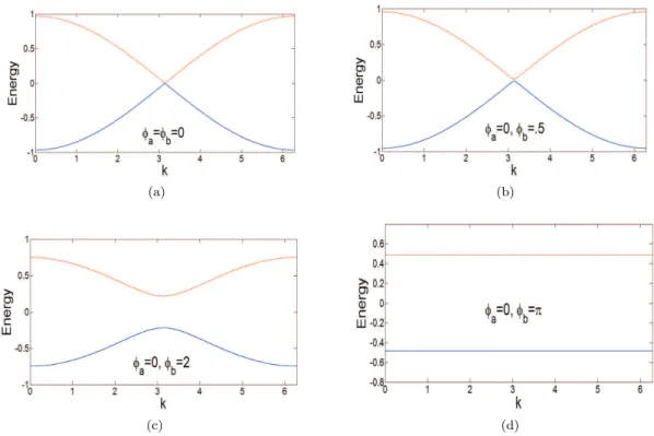
FIG. 6: Energy bands for the system shown in Fig. 5. The band gap vanishes when the two phases are equal (a) and opens up when the two phase values differ. The gap is still very small in (b), but grows as|φa−φb|increases (c), reaching its maximum
size when|φa−φb|=π(d).
are independent of k, as in the usual SSH case, then ∆ = 2|v−w|, but notice that in the present casev and
w depend on momentum via thek-dependent transmit-tances. In this sense, this is not the true SSH model, but a slight variant of it, which we might call the modified SSH (MSSH) model; this is a continuous deformation of the usual SSH model and so should have topologically identical behavior, as will be verified below.
The nonvanishing coefficients of the Pauli matrices in Eq. 5 are now
dx(k) = |ta(k)|+|tb(k)|cosk (14)
dy(k) = |tb(k)|sink. (15)
As k goes from 0 to 2π, d traces out paths labeled by
their winding numbersν about the origin. These wind-ing numbers will be functions of the hoppwind-ing amplitudes:
ν(v, w) = ν(|ta|,|tb|). Since ta and tb vary only weakly
withk, it is clear that the loop traced out byd(k) encloses
the origin and has nonzero winding number if|tb|>|ta|.
B. Verifying topological behavior: localized boundary states.
Properties of the system of Fig. 5 can be numeri-cally simulated, and the results verify that the model constructed here has behavior similar to that expected
from the SSH model. Fig. 6 shows plots of the energy levels for different values of the phase shiftsφa andφb of
the two graphs. When the two phase shifts are equal, the band gap vanishes. As they begin to differ, a gap opens up and becomes larger with increasing|φa−φb|,
reach-ing a maximum at|φa−φb|=π, as Fig. 6 shows. The
exact shapes of the curves are slightly different than the pure SSH model (in particular, the value ofkthat mini-mizes the gap clearly shifts horizontally as the parameter changes), but the qualitative behavior is identical.
Similarly, it is easy to show that different values of the phase shifts allow solutions with both zero and nonzero winding numbers to occur. Evaluation of Eqs. 9, 14, and 15 for a range ofφaandφbvalues readily shows that
vary-ing these phases causes the path traced out bydto shift
horizontally and change radius, leading to transitions be-tween winding numbers 0 and 1. This indicates that ferent phase values in the two diamond graphs lead to dif-ferent topological phases, distinguished by their winding numbers. By attaching two chains of these graphs with different winding numbers on each chain there should then arise localized, topologically-protected states at the boundaries between them [15–17].
Fig. 7 supports this analysis by showing specific con-ditions under which topologically protected states can be generated using a network of multiports. The plots compare two numerical simulations of a single photon quantum walk on the MSSH model described above for
1.00 0.50 0.00 0.2500 0.1250 0.000 0.140 0.070 0.000 0.04500 0.02250 0.000 -75 0 74 -75 0 74 m m
Probability to be found at position
m 1.00 0.50 0.00 0.2500 0.1250 0.000 0.180 0.090 0.000 0.180 0.090 0.000
Coordinate indexmover cells
t=0 t=0 t=60 t=120 t=200 t=60 t=120 t=200
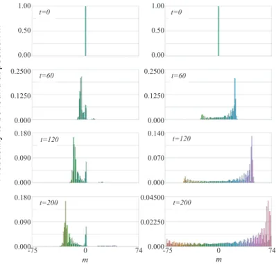
FIG. 7: Comparison of MSSH quantum walk with topologically protected edge state (left) and MSSH quantum walk with normal ballistic spreading (right) for 0≤t≤200. The two walks are simulated for the arrangement shown in Fig. 5. The topology on the left uses (φa= 1.5, φb= 2.5) whenm≤0, giving a winding numberν 6= 0; this joins up with aν= 0 region
having phase shifts of (φa = 3π/4, φb = 0) when m ≥0. The result is a localized state confined to the boundary of these
topologies, indicated by the peak that arises atm= 0. In contrast, the topology on the right usesφa = 0, φb= 0 for allm,
leading to a ballistic quantum walk in one dimension.
0 ≤ t ≤ 200 in units of T. In each case an initially right-moving photon is injected at subsiteaof them= 0 position coordinate att= 0 (top row). (The mechanism for physically inserting photon states into the chain is described in detail in Ref. [31].) The left hand column shows the time evolution over a chain with two different topologies attached to each other at m = 0. The right hand side shows time evolution over a chain with uniform topology.
Specifically, the left column of Fig. 7 uses subsite phase shifts ofφa = 1.5, φb= 2.5 for the portion to the left of
the origin (m ≤ 0), giving a winding number ν 6= 0 in that region. To the right of the origin (m ≥ 0), phase shifts of φa = 3π/4, φb= 0 are used, giving ν = 0. The
result is a persistent probability of finding the photon at the boundary between the two topologies, the signature of a topologically protected edge state [16].
For comparison, the right column of Fig. 7 shows a quantum walk over the MSSH model using no change in phase shifts: φa = 0, φb = 0 for all m (positive and
negative). As expected, in this case evolution reduces to a standard quantum walk in one dimension, exhibiting ballistic spreading of probability over the coordinates.
Note that the right side of Fig. 7 is asymmetric. This is because the valueφa =φb that was used reduces the
lattice to a chain of three-ports with transition matrix of form Eq. 2; this matrix has much smaller amplitude to reflect out the input port than to transmit out the other two, resulting in a strong bias of the photon to continue moving in its initial direction. For other values ofφa or
φb (or for other values of the internal vertex phase θ of
Eq. 1) this bias changes or disappears.
It may also be pointed out that the diamond graphs have four bound states [35] whenφa−φb= 0, and none
for φa −φb 6= 0. These bound states occur in all the
diamond graphs at exactly at the parameter valuesφa =
φb = 0 at which the energy gap closes. This allows the
controlled storage of photons: photons can be stored in the graph or released as the value ofφis changed.
V. CONCLUSIONS
Systems with distinct topological phases are of increas-ing importance in condensed matter physics and in quan-tum computing. The ability to simulate their properties
8
in a simple manner is therefore of current interest, and the ability to supply such simulations efficiently using only linear optical quantum systems would be a useful advance. Here, a method for simulation of systems in the same topological class as the SSH Hamiltonian was proposed that for large numbers of time steps requires substantially fewer resources than the method of [30].
In this paper the focus was on the use of only one-dimensional chains of directionally-unbiased optical three-ports. However, this only scratches the surface of the possibilities to be examined, since the current ap-proach can be generalized to two- and three-dimensional arrays of n-ports with n > 3. The phase shifts at each vertex of the multiport can also be varied, altering the
multiport properties. Thus a rich array of more sophisti-cated simulation types remains as-yet unexplored, using the same general methods. These hold promise to pro-vide quantum simulation of a diverse range of further phenomena.
Acknowledgements
This research was supported by the National Science Foundation EFRI-ACQUIRE Grant No. ECCS-1640968, NSF Grant No. ECCS- 1309209, and by the Northrop Grumman NG Next.
[1] M. A. Nielsen and I. L. Chuang, Quantum Computa-tion and Quantum InformaComputa-tion(Cambridge Univ. Press, Cambridge, 2001).
[2] K. A. Yu, A. H. Shen,and M. N. Vyalyi M N,Classical and Quantum Computation(American Mathematical So-ciety, Providence, 2002).
[3] G. Jaeger, Quantum Information: An Overview
(Springer, Berlin, 2006).
[4] G. Falci and E. Paladino,Int. J. Quant. Inf.12, 1430003 (2014).
[5] R. P. Feynman,Int. J. Theor. Phys. 21467 (1982). [6] A. Aspuru-Guzi and P. Walther, Nat. Phys. 8, 285
(2012).
[7] T. H. Johnson, S. R. Clark and D. Jaksch,EPJ Quantum Technology 1, 10 (2014).
[8] R. P. Feynman,Rev. Mod. Phys.20, 367 (1948). [9] R. P. Feynman, A. R. Hibbs, D. F. Styer,Quantum
Me-chanics and Path Integrals (Dover, Mineola, NY, 2010). [10] J. Kempe,Contemp. Phys.44, 307 (2003).
[11] S. E. Venegas-Andraca,Quant. Inf Proc.11, 1015 (2012). [12] Y. Shih,Rep. Prog. Phys.66, 1009 (2003).
[13] Z. Y. J. Ou, Multi-Photon Quantum Interference
(Springer, Berlin, 2007).
[14] D. S. Simon, G. Jaeger, A. V. Sergienko, Quan-tum Metrology, Imaging, and Communication(Springer, Berlin, 2017).
[15] M. Z. Hasan and C. L. Kane,Rev. Mod. Phys.82, 3045 (2010).
[16] T. Kitagawa,Quant. Inf. Proc.11, 1107 (2012). [17] J. K. Asb´oth, L. Oroszl´any, and A. P´alyi,A Short Course
on Topological Insulators (Springer, Berlin, 2016). [18] B. A. Bernevig, T. L. Hughes, Topological Insulators
and Topological Superconductors (Princeton University Press, Princeton, 2013).
[19] T. D. Stanescu, Introduction to Topological Matter and Quantum Computation (CRC Press, Boca Raton, 2017). [20] J. Ruostekoski, G. V. Dunne, and J. Javanainen, Phys.
Rev. Lett.88, 180401 (2002).
[21] J. Ruostekoski, J. Javanainen, and G. V. Dunne, Phys. Rev. A77, 013603 (2008).
[22] X.-J. Liu, Z.-X. Liu, andM. Cheng, Phys. Rev. Lett. 110, 076401 (2013).
[23] X. Li, E. Zhao, and W. V. Liu, Nat. Commun.4, 1523 (2013).
[24] J. Javanainen and J. Ruostekoski, Phys. Rev. Lett.91, 150404 (2003).
[25] D.-W. Zhang, L.-B. Shao, Z.-Y. Xue, H. Yan, Z. D. Wang, and S.-L. Zhu, Phys. Rev. A86, 063616 (2012). [26] D.-W. Zhang, F. Mei, Z.-Y. Xue, S.-L Zhu, and Z. D.
WangPhys. Rev. A92, 013612 (2015).
[27] M. A. Broome, A. Fedrizzi, B. P. Lanyon, I. Kassal I, A. Aspuru-Guzik, and A. G. White,Phys. Rev. Lett. 104, 153602 (2010).
[28] T. Kitagawa, M. S. Rudner, E. Berg, and E. Demler
Phys. Rev. A82, 033429 (2010).
[29] T. Kitagawa, E. Berg, M. Rudner, and E. Demler,Phys. Rev. B.82, 235114 (2010).
[30] T. Kitagawa, M. A. Broome, A. Fedrizzi, M. S. Rudner, E. Berg, I. Kassal, A. Aspuru-Guzik, E. Demler, A. G. White,Nature Comm.3, 882 (2012).
[31] D. S. Simon, C. A. Fitzpatrick, S. Osawa, and A. V. Sergienko,Phys. Rev. A95042109 (2017).
[32] D. S. Simon, C. A. Fitzpatrick and A. V. Sergienko,Phys. Rev. A93, 043845 (2016).
[33] M. Hillery, J. Bergou, and E. Feldman,Phy. Rev. A68 032314 (2003).
[34] E. Feldman and M. Hillery,Phy. Lett. A,324277 (2004). [35] E. Feldman and M. Hillery,Cont. Math.,38171 (2005). [36] E. Feldman and M. Hillery,J. Phys. A: Math. Theor.40,
11343 (2007).
[37] A. Slobozhanyuk, S. H. Mousavi, X. Ni, D. Smirnova, Y. S. Kivshar, A. B. Khanikaev,Nat. Phot.11, 130 2016. [38] W. P. Su, J. R. Schrieffer, and A. J. Heeger,Phys. Rev.
B 22, 2099 (1980).
[39] R. Jackiw and C. Rebbi,Phys. Rev. D 13, 3398 (1976). [40] H. Obuse and N. Kawakami, Phys. Rev. B 84, 195139
(2011).
[41] J. K. Asb´oth, Phys. Rev. B86, 195414 (2012).
[42] J. K. Asb´oth and H. Obuse, Phys. Rev. B 88, 121406 (2013).
[43] J. K. Asb´oth and J. M. Edge, Phys. Rev. A91, 022324 (2015).