Tree Automata Completion for Static Analysis of
Functional Programs
Thomas Genet, Yann Salmon
To cite this version:
Thomas Genet, Yann Salmon. Tree Automata Completion for Static Analysis of Functional Programs. 2013. <hal-00780124v2>
HAL Id: hal-00780124
https://hal.archives-ouvertes.fr/hal-00780124v2
Submitted on 27 May 2013HAL is a multi-disciplinary open access archive for the deposit and dissemination of sci-entific research documents, whether they are pub-lished or not. The documents may come from teaching and research institutions in France or abroad, or from public or private research centers.
L’archive ouverte pluridisciplinaire HAL, est destin´ee au d´epˆot et `a la diffusion de documents scientifiques de niveau recherche, publi´es ou non, ´emanant des ´etablissements d’enseignement et de recherche fran¸cais ou ´etrangers, des laboratoires publics ou priv´es.
Tree Automaton Completion for Static
Analysis of Functional Programs
Thomas Genet
∗Yann Salmon
†May 24, 2013
Tree Automata Completion is a family of techniques for computing or approxi-mating the set of terms reachable by a rewriting relation. For functional programs translated into TRSs, we give a sufficient condition for completion to terminate. Second, in order to take into account the evaluation strategy of functional pro-grams, we show how to refine completion to approximate reachable terms for a rewriting relation controlled by a strategy. In this paper, we focus on innermost strategy which represents the call-by-value evaluation strategy.
1 Introduction
Computing or approximating the set of terms reachable by rewriting finds more and more applications. For a Term Rewriting System (TRS)Rand a set of termsL0⊆T(Σ), the set of reachable terms isR∗(L0) = n t∈T(Σ) ∃s∈L0, s→ ∗ Rt o
. This set can be computed for specific classes ofRbut, in general, it has to be approximated. Applications of the approximation of
R∗(L0) are ranging from cryptographic protocol verification [GK00, ABB+05], to static analysis
of various programming languages [BGJL07, KO11] or to TRS termination proofs [Mid02, GHWZ05]. Most of the techniques compute such approximations using tree automata as the core formalism to represent or approximate the (possibly) infinite set of termsR∗(L0). Most
of them also rely on a Knuth-Bendix completion-like algorithm to produce an automaton A∗recognising exactly, or over-approximating, the set of reachable terms. As a result, these techniques can be refered as tree automata completion techniques [Gen98, TKS00, Tak04, FGVTT04, BCHK09, GR10, Lis12].
In this paper, we investigate the application of tree automata completion techniques to the static analysis of functional programs. The objective of such an analysis is to over-approximate the set of possible results of higher-order functional programs [OR11, KO11]. First, like the standard Knuth-Bendix completion, tree automata completion is not guaranteed to terminate. For TRSs extracted from functional programs, we show that termination of automata comple-tion is guaranteed using natural constraints on the definicomple-tion of the approximacomple-tion. Second, we show that completion can take the rewriting strategy into account, i.e. over-approximate
∗
IRISA, Campus de Beaulieu, 35042 Rennes Cedex, France,[email protected]
†
terms reachable by rewriting under a strategy. In this paper, we focus on the innermost strat-egy which corresponds to the call-by-value stratstrat-egy that is at the heart of several functional programming languages, such as Ocaml [LDG+12].
Surprisingly, very little effort has been done on computing or over-approximatingR∗strat(L0),
i.e. set of reachable terms whenRis applied with a strategystrat. To the best of our knowledge, Pierre RÃľty’s work [RV02] is the only one to have tackled this goal. He gives some sufficient conditions onL0andRforR
∗
strat(L0) to be recognised by a tree automatonA
∗
, wherestratcan be the innermost or the outermost strategy. However, those restrictions onRandL0are strong
and generally incompatible with the analysis of functional programs. In this paper, we define a tree automata completion algorithm over-approximating the setR∗in(L0) for all left-linear
TRSsRand all regular set of input termsL0.
This paper is organised as follows: Section 2 recalls some basic notions about TRSs and tree automata. Section 3 defines tree automata completion. Section 4 shows how to guarantee the termination of completion when analysing TRSs obtained from functional programs. Section 5 presents some experiments. Finally, Section 6 explains how to tune completion so as to take innermost strategy into account.
2 Basic notions and notations
2.1 TermsDefinition 1 (Signature).
A signature is a set whose elements are called function symbols. Each function symbol has an arity, which is a natural integer. Function symbols of arity 0 are called constants. Given a signatureΣandk∈N, the set of its function symbols of aritykis notedΣk. 1J Definition 2 (Term, ground term, linearity).
Given a signatureΣand a setX whose elements are called variables and such thatΣ∩ X =∅, we define the set of terms overΣ andX,T(Σ,X), as the smallest set such that :
1. X ⊆T(Σ,X) and
2. ∀k∈N,∀f ∈Σk,∀t1, . . . , tk∈T(Σ,X), f(t1, . . . , tk)∈T(Σ,X).
Terms in which no variable appears, i.e. terms inT(Σ,∅), are called ground; the set of ground terms is notedT(Σ).
Terms in which any variable appears at most once are called linear.1 2J Definition 3 (Substitution).
A substitution overT(Σ,X) is an application fromX toT(Σ,X). Any substitution is induc-tively extended toT(Σ,X) byσ(f(t1, . . . , tk)) =f(σ(t1), . . . , σ(tk)). Given a substitutionσ and a
termt, we notetσ instead ofσ(t). 3J
Definition 4 (Context).
A context overT(Σ,X) is a term inT(Σ∪ X,{}) in which the variableappears exactly once. A ground context overT(Σ,X) is a context overT(Σ). The smallest possible context,, is called the trivial context. Given a contextC and a termt, we noteC[t] the termCσt, where
σt:7→t. 4J
Definition 5 (Position).
Positions are finite words over the alphabet N. The set of positions of term t, Pos(t), is defined by induction overt:
1. for all constantcand all variableX, Pos(c) = Pos(X) ={Λ}and 2. Pos(f(t1, . . . , tk)) ={Λ} ∪
k [
i=1
{i}.Pos(ti). 5J
Definition 6 (Subterm-at-position, replacement-at-position).
The position of the hole in contextC, Pos(C), is defined by induction onC: 1. Pos() =Λ
2. Pos(f(C1, . . . , Ck)) =i.Pos(Ci), whereiis the unique integer inJ1 ;kKsuch thatCiis a
context.
Given a term u and p ∈ Pos(u), there is a unique context C and a unique term v such that Pos(C) =pandu =C[v]. The termv is notedu|p, and, given another termt, we note
u[t]p=C[t]. 6J
2.2 Rewriting
Definition 7 (Rewriting rule, term rewriting system).
A rewriting rule over (Σ,X) is a couple (`, r)∈T(Σ,X)×T(Σ,X), that we note`→r, such that any variable appearing inralso appears in`. A term rewriting system (TRS) over (Σ,X) is
a set of rewriting rules over (Σ,X). 7J
Definition 8 (Rewriting step, redex, reducible term, normal form).
Given a signature (Σ,X), a TRSRover it and two termss, t∈T(Σ), we say thatscan be rewritten intotbyR, and we notes→Rtif there exist a rule`→r∈R, a ground contextC overT(Σ) and a substitutionσ overT(Σ,X) such thats=C[`σ] andt=C[rσ].
In this situation, the termsis said to be reducible byRand the subterm`σ is called a redex ofs. A termsthat is not reducible byRis a normal form ofR. The set of normal forms ofRis noted Irr(R).
We note→∗
Rthe reflexive and transitive closure of→R. 8J Definition 9 (Set of reachable terms).
Given a signature (Σ,X), a TRS R over it and a set of terms L⊆ T(Σ), we note R(L) = {t∈T(Σ)| ∃s∈L, s→Rt}andR∗(L) =nt∈T(Σ) ∃s∈L, s→ ∗ Rt o . 9J Definition 10 (Left-linearity).
A TRSRis said to be left-linear if for each rule`→rofR, the term`is linear. 10J Definition 11 (Constructors and defined symbols, sufficient completeness).
Given a TRSRover (Σ,X), there is a partition (C,D) ofΣ such that all symbols occurring at the root position of left-hand sides of rules ofRare inD. Dis the set of defined symbols ofR,Cis the set of constructors. Terms inT(C) are called data-terms. A TRSRover (Σ,X) is sufficiently complete if for alls∈T(Σ),R∗({s})∩T(C),∅. 11J
2.3 Equations
Definition 12 (Equivalence relation, congruence).
A binary relation over some setS is an equivalence relation if it is reflexive, symmetric and transitive.
An equivalence relation≡overT(Σ) is a congruence if for allk∈N, for allf ∈Σk, for all
t1, . . . , tk, s1, . . . , sk∈T(Σ) such that∀i∈J1 ;kK,ti≡si, we havef(t1, . . . , tk)≡f(s1, . . . , sk). 12J
Definition 13 (Equation,≡E).
An equation over (Σ,X) is a pair of terms (s, t)∈T(Σ,X)×T(Σ,X), that we notes=t. A setE of equations over (Σ,X) induces a congruence≡EoverT(Σ) which is the smallest congruence overT(Σ) such that for alls=t∈Eand for all substitutionθ:X →T(Σ),sθ≡
Etθ. The classes
of equivalence of≡Eare noted with [·]E. 13J
Definition 14 (Rewriting moduloE).
Given a TRSRand a set of equationsEboth over (Σ,X), we define theRmoduloErewriting relation,→R/E, as follows. For anyu, v∈T(Σ),u→R/Evif and only if there existu0, v0∈T(Σ) such thatu0≡Eu,v0≡Evandu0→Rv0.
We define→∗
R/E, (R/E)(L) and (R/E) ∗
(L) forL⊆T(Σ) as in Definitions 8 and 9. 14J 2.4 Tree automata
Definition 15 (Tree automaton, delta-transition, epsilon-transition, new state).
An automaton overΣis someA= (Σ, Q, QF, ∆) whereQis a finite set of states,QFis a subset ofQwhose elements are called final states and∆a finite set of transitions. A delta-transition is of the formf(q1, . . . , qk)q 0 wheref ∈Σ k andq1, . . . , qk, q 0 ∈Q. An epsilon-transition is of the formqq0 whereq, q0∈Q. A configuration ofAis a term inT(Σ, Q).
A stateq∈Qthat appears nowhere in∆is called a new state. A configuration is elementary if each of its subconfigurations at depth 1 (if any) is a state. A configuration is trivial if it is
just a state. 15J
Remark. We simply writeAto denote an automaton, writeQAfor the set of states ofA. We assimilate an automaton with its set of transitions. When taking a “new state”, we silently expandQAif needed. We are only rarely interested inQF, the set of final states.
Definition 16.
LetA= (Σ, Q, QF, ∆) be an automaton and letc, c0 be configurations ofA. We say thatA recognisescintoc0in one step, and notec
A c 0
if there a transitionτρinAand a context
CoverT(Σ, Q) such thatc=C[τ] andc0=C[ρ]. We note∗
A the reflexive and transitive closure
of
A and, for anyq
∈Q,L(A, q) = t∈T(Σ) t∗ A q
. We extend this definition to subsets of
Qand noteL(A) =L(A, QF). 16J
Definition 17 (Determinism, Completeness).
An automaton is deterministic if it has no epsilon-transition and for all delta-transitions
τρandτ0 ρ0, ifτ=τ0 thenρ=ρ0. An automaton is complete if each of its non-trivial configurations is the left-hand side of some of its transitions. 17J
Definition 18 (Colours).
Transitions may have “colours”, likeRfor transition qR q0, and we denote byAR the automaton obtained fromAby removing all transitions coloured withR. 18J Definition 19.
Given two statesq,q0 of some automatonAand a colourE, we noteq
E A q0 when we have bothqE A q 0 andq0E A q. 19J Remark. q E, ∗ A q0 is stronger than (qE,∗ A q 0 ∧q0 E,∗ A q). E,∗ A
is an equivalence relation overQA. This relation is extended to a congruence relation overT(Σ, Q). The equivalence classes are noted with [·]E.
Definition 20.
LetA= (Σ, Q, QF, ∆) be an automaton andEa colour. We noteA/Ethe automaton overΣ whose set of states isQ/E, whose set of final states ifQF/Eand whose set of transitions is
n f([q1]E, . . . ,[qk]E) q0 E f(q1, . . . , qk)q 0 ∈∆o ∪n[q] E q0 E qq 0 ∈∆∧[q] E, q0 E o . 20J
Remark. For any configurationsc, c0 ofA, we havec∗ A c 0 if and only if [c]E ∗ A/E c0 E. So the languages recognised byAandA/Eare the same.
We now give notations used for pair automata, the archetype of which is the product of two automata.
Definition 21 (Pair automaton).
An automatonA= (Σ, Q, QF, ∆) is said to be a pair automata if there exists some setsQ1and
Q2such thatQ=Q1×Q2. 21J
Definition 22 (Product automaton).
LetA= (Σ, Q, QF, ∆A) andB= (Σ, P , PF, ∆B) be two automata. The product automaton ofA andBisA × B= (Σ, Q×P , QF×PF, ∆) where ∆=nf(hq1, p1i, . . . ,hqk, pki) q0, p0 f(q1, . . . , qk)q 0 ∈∆A∧f(p1, . . . , pk)p0∈∆Bo ∪nhq, pi q0, p0 qq 0 ∈∆Ao∪nhq, pi q, p0 pp 0 ∈∆Bo. 22J Definition 23 (Projections).
LetA= (Σ, Q, QF, ∆) be a pair automaton, letτ ρbe one of its transitions andhq, pibe one of its states. We define Π1(hq, pi) =q and extend Π1(·) to configurations inductively:
Π1(f(γ1, . . . , γk)) =f(Π1(γ1), . . . , Π1(γk)). We defineΠ1(τρ) =Π1(τ)Π1(ρ). We define
Π1(A) = (Σ, Π1(Q), Π1(QF), Π1(∆)).Π2(·) is defined on all these objects in the same way for
the right components. 23J
Remark. UsingΠ1(A) amounts to forgetting the precision given by the right components of
2.5 Innermost strategies
In general, a strategy over a TRS R is a set of (computable) criteria to describe a certain subrelation of→R. In this paper, we will be interested in innermost strategies. In these strate-gies, commonly used to execute functional programs (“call-by-value”), terms are rewritten by always contracting one of the lowest reducible subterms.
Definition 24 (Innermost strategy).
Given a TRSRand two termss, t, we say thatscan be rewritten intotbyRwith an innermost strategy, and we notes→R
int, ifs→Rtand each strict subterm of the redex insis aR-normal form. We define→∗
Rin,Rin(L) andR ∗
in(L) as in Definitions 8 and 9. 24J
Remark. It is in fact sufficient to check whether subterms ofsat depth 1 are in normal form to decide whetherscan be rewritten with an innermost strategy.
To deal with innermost strategies, we will have to discriminate normal forms. This is possible within the tree automaton framework whenRis left-linear.
Theorem 25 ([CR87]).
LetRbe a left-linear TRS. There is a deterministic and complete tree automatonIRR(R) such thatL(IRR(R)) = Irr(R) and with a distinguished statep
redsuch thatL(IRR(R), pred) =
T(Σ)rIrr(R). 25
Remark. From determinism and the property ofpred follows that for any state pdifferent
frompred,L(IRR(R), p)⊆Irr(R).
3 Classical equational completion
Equational completion of [GR10] is an iterative process on automata that is not guaranteed to terminate. Each iteration comprises two parts: (exact) completion itself, then equational merging. The former tends to incorporate descendants byR of already recognised terms into the recognised language; this leads to the creation of new states. The latter tends to merge states in order to ease termination of the overall process, at the cost of precision of the computed result. Some transition added by equational completion will have coloursRorE; it is assumed that the transitions of the input automatonA0do not have any colour and thatA0 does not have any epsilon-transition.
3.1 Exact completion
Exact completion is about resolving critical pairs. A critical pair represents a situation where some term is recognised by the current automaton, but not its descendants byR. Its resolution consists in adding transitions to let the descendants be recognised as well. This process can create new critical pairs.
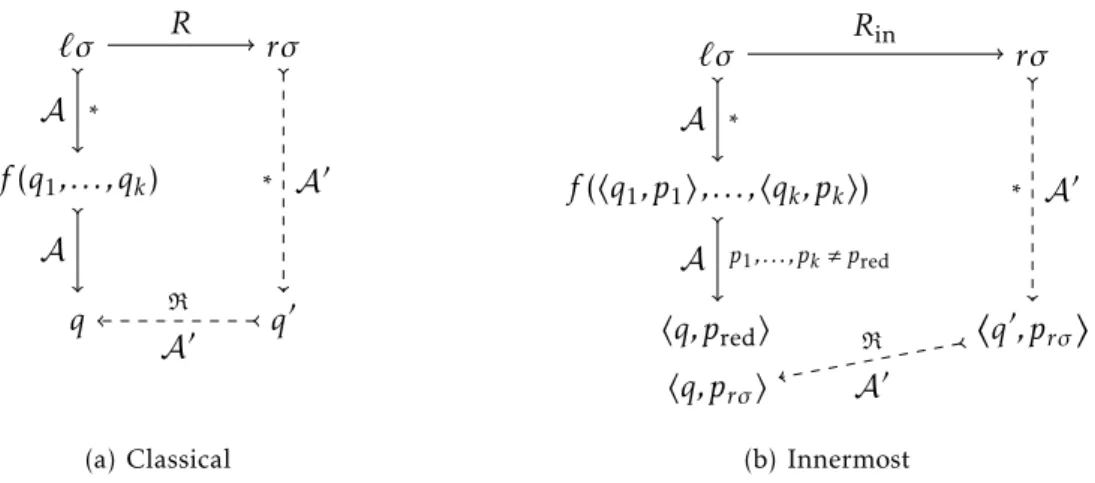
Definition 26 (Critical pair).
A pair (`→r, σ , q) where`→r∈R,σ :X →QAandq∈QAis critical if (see Figure 1(a)) 1. `σ∗
2. rσ ∗ A q. 26J We will want to add transitionsrσ q0 andq0 q0. However, doing the former is not generally possible in one step, asrσ might be a non-elementary configuration. We will have to normalise this configuration by adding intermediate states. For example, to setf(g(a, b))q0, we will first addaqa, then,bqb,g(qa, qb)qgand finallyf(qg)q0, exploringf(g(a, b)) with a postfix traversal. At each of these steps, we will look whether we could reuse an already existing transition; if not, we will add a new state.
Definition 27 (NormA(c, q)).
LetAbe an automaton,cbe a non-trivial configuration andqbe any state. LetΞ= (ξ1, . . . , ξK) be a postfix traversal ofc(ξK is the root position). With∆the set of transitions ofA, let us use an auxiliary function:
NormA(c, q) =NormAuxΞ,∆1(c, q). (1) Now let us defineNormAux·Ξ,i. Foriranging from 1 toK−1, for any set of transitions∆and any configurationdsuch thatd|ξi is an elementary configuration, let
NormAuxΞ,i∆ (d, q) ={d|ξ i q 0 } ∪NormAuxΞ,i+1 ∆∪{d|ξiq0}(d q0 ξi, q) (2)
whereq0 is such thatd|ξi q 0
in∆/E(or, if there is no such state,q0is a new state, distinct from
q). Also, for any set of transitions∆and any elementary configurationd, let
NormAuxΞ,K∆ (d, q) ={dq}. (3) 27J Remark. It is necessary to consider equivalence byEwhen searching for an already existing transition. Suppose we work with somef(q1) and haveq1E
∆
q2 andf(q2)
∆ q
0
: we do not want to create a new state here, but reuseq0 and setf(q1)q
0 . Definition 28 (Completion of a critical pair).
A critical pairCP = (` →r, σ , q) in automatonA is completed by first computing N =
NormA
R(rσ , q
0
) whereq0 is a new state, then adding toAthe new states and the transitions appearing inN as well as the transitionq0R q. Ifrσ is a trivial configuration (ie. ris just a
variable), only transitionrσ R qis added. 28J
`σ rσ q q0 R A ∗ ∗ A0 A0 R
(a) A critical pair
sθ tθ q1 q2 E A ∗ ∗ A E A0 (b) Situation of ap-plication
Definition 29 (Step of completion).
The automaton resulting from completion of a list comprising of one critical pairCP is notedJ(CP)
R (A). For a list of zero critical pair, we set J
()
R (A) = A and for any listLCP of critical pairs (ofA) whose head isCP and tail isLCP0,JLCP
R (A) =JLCP 0 R J(CP) R (A) . A step of completion of automatonAconsists in producing automatonCR(A) =JCP
R (A), whereCP is a
list of all critical pairs ofA. 29J
Example 30.
LetΣ be defined with Σ0 ={n,0}, Σ1 = {s, a, f}, Σ2 ={c} where 0 is meant to represent
integer zero,sthe successor operation on integers,athe predecessor (“antecessor”) operation,
nthe empty list,cthe constructor of lists of integers andf intended by some unwise person to be the function on lists that filters out integer zero. LetR ={f(n)→n, f(c(s(X), Y)) →
c(s(X), f(Y)), f(c(a(X), Y))→ c(a(X), f(Y)), f(c(0, Y))→f(Y), a(s(X)) →X, s(a(X))→X}. Let A0={nqn,0q0, s(q0)qs, a(qs)qa, c(qa, qn)qc, f(qc)qf}.
We haveL(A0, qf) ={f(c(a(s(0)), n))}andR(L(A0, qf)) ={f(c(0, n)), c(a(s(0)), f(n))}.
There is a critical pairCP1inA0with the rulef(c(a(X), Y))→c(a(X), f(Y)), the substitution
σ1 ={X 7→ q
s, Y 7→ qn} and the state qf. It is resolved by adding transitions to recognise
c(a(qs), f(qn)) intoqf. Normalisation finds and reuses the transitiona(qs)qa. It has to create a new stateqN1 such that f(qn)qN1, and qN2 such that c(qa, qN1) qN2. We then add
qN2
R
qf, and have producedJ
(P C1) R (A0).
Another critical pair isCP2inA0with the rulea(s(X))→X, the substitutionσ2={X7→q0}
and the stateqa. It is resolved by adding toJ
(P C1) R (A0) the transitionq0 R qa, producing J(P C1,P C2) R (A0).
There is no more critical pair inA0: thusCR(A0) =J(P C1,P C2)
R (A0). There is a new critical
pair inCR(A0) withf(n)→n, the empty substitution and stateqN1. 30C 3.2 Equational merging
Since completion of a critical pair can create new critical pairs, the process fuels itself, which is problematic for obtaining a fix-point. Equational merging is a way of countering this phenomenon at the cost of precision that is parametrised by equations overT(Σ).
Definition 31 (Situation of application of an equation).
Given an equations=t, an automatonA, aθ:X →QAand statesq1andq2, we say that (s=t, θ, q1, q2) is a situation of application inAif (see Figure 1(b))
1. sθ∗ A q1, 2. tθ∗ A q2 and 3. q1 E A q2. 31J
Definition 32 (Application of an equation).
Given (s=t, θ, q1, q2) a situation of application inA, applying the underlying equation in it
consists in adding transitionsq1
E
q2andq2
E
q1toA. This produces a new automatonA
0
and we noteA;EA0. 32J
Remark. In [GR10],q1andq2were merged by “renaming”q2intoq1, ie. removingq2from
QA and replacing every occurrence ofq2byq1in the transitions ofA. This is equivalent to applying our method, then considering automatonA/E(see definition 20) and finally choosing a representative (hereq1for the class{q1, q2}) of each equivalence class of states.
Definition 33 (Simplified automaton).
Given an automatonAand a set of equationsE, we call simplified automaton ofAbyEand noteSE(A) the automaton resulting from the successive application of all applicable equations
inA. 33J
Remark (;Eis confluent). Indeed, there is a unique automatonA!that differs fromAonly by itsE-transitions and is suchAR;∗
E(A!)R and there is no more situation of application of equations in (A!)R.
Definition 34 (Step of equational completion).
A step of equational completion is the composition of a step of exact completion, then equational simplification:CER,E(A) =SE(CR(A)). 34J The following notion is part of an easier discourse about theR/E-coherence notion of [GR10]. Definition 35 (Coherent automaton).
LetA0= (Σ, Q, QF, ∆) be a tree automaton andEa set of equations. The automatonA0is said to beE-coherentif for allq∈Q, there existss∈L(A0, q) such thatL(A0, q)⊆[s]E. 35J 3.3 Known results
We now recall the two main theorems of [GR10]. Theorem 36 (Correctness).
LetA0be some automaton. Assume the equational completion procedure defined above terminates when applied toA0. LetA∗be the resulting fix-point automaton. IfRis left-linear, then the calculated over-approximation is correct, that is
L(A∗)⊇R∗(L(A0)). 36 We will make usage ofE-coherence for the precision theorem.
Lemma 37.
LetA0be a E-coherent automaton, Ra left-linear TRS andA be an automaton obtained fromA0after several steps of equational completion withR, E. ThenARisE-coherent and moreover, for all stateqofA, there existss∈L(AR, q) such thatL(A, q)⊆(R/E)∗(s). 37 Such an automaton is said to beR/E-coherent. The intuition behind this is the following: in the tree automaton,R-transitions represent rewriting steps and transitions ofARrecognize
are recognized into the same stateqinARthen they belong to the sameE-equivalence class. Otherwise, if at least oneR-transition is necessary to recognize, say,tintoqthen at least one step of rewriting was necessary to obtaintfroms. In [GR10], the following theorem made an assumption ofR/E-coherence forA0, but, given thatA0does not have anyR-transition,A0is
R/E-coherent if and only if it isE-coherent. Theorem 38 (Upper bound).
LetEbe a set of equations,A0aE-coherent tree automaton andRa left-linear TRS. IfAis an automaton produced fromA0after several steps of equational completion withR, E, then
L(A)⊆(R/E)∗(L(A0)) 38
4 Termination of completion for functional programs
Now, we consider functional programs viewed as TRSs. We assume that such TRSs are left-linear, which is a common assumption on TRSs obtained from functional programs [BN98]. In this section, we will restrict ourselves to sufficiently complete constructor-based TRSs and will refer to them asfunctional TRSs. For the moment, types used in the functional program are not taken into account in the TRS, but they will be in a next section. First, we state a sufficient condition for completion to terminate and, next, we will specialize it for functional TRS. Remark. In this section, we will be interested in counting the states of A/E, where A is produced by equational completion. As we remarked just after definition 32, dealing with A/E amounts to act as if applying an equation would effectively merge (or rename) states. Therefore, we will assimilateA/EwithAand consider that states in relation modulo E,
∗ A
are merged. Note that with this convention,AR(that is indeed (A/E)R) has no epsilon-transition. 4.1 Ensuring termination of completion
In this section, we show that ifT(Σ)/≡
E is finite then completion terminates by proving that completion produces no more new states thanE-equivalence classes. Doing so is not possible for an arbitraryEbecause equational completion does not take reflexivity of≡E into account and there may existq,q0such thats
A qandsA q 0
.2We will enrichEwith a set of reflexivity equations that solve this difficulty without altering≡E.
Definition 39 (Set of reflexivity equationsEr).
For a given set of symbolsΣ,Er={f(x1, . . . , xk) =f(x1, . . . , xk)|k∈N∧f ∈Σk}. 39J Note that for all set of equationsE, the relation≡Eis the same as≡E∪Er. However, simpli-fication withEr transforms all automaton into an automatonAwhose states coincide with equivalence classes of≡Eand such thatARis deterministic, as stated in the following lemmas.
Lemma 40.
LetAbe some automaton,s=tbe some equation ofE andθ:X →QA. Ifsθ ∗
SE(A)qand tθ ∗ SE(A)q 0 , thenq ∗ SE(A)q 0 orq0 ∗ SE(A)q. If S
E(A) has no epsilon-transition, thenq=q 0
. 40
Proof.
This translates the fact that, by definition, there cannot be a situation of application for equations=tinSE(A), and we chose a representation of automata where states in relation moduloE, ∗ A are merged. Lemma 41.
For all tree automatonAwithout epsilon-transition and all set of equationsE, ifE⊇Er, thenS
E(A) is deterministic. 41
Proof.
SinceAhas no epsilon-transition, neither doesS
E(A). We prove this lemma by induction on the terms recognized bySE(A). Letabe a constant such thata ∗
SE(A)qanda ∗ SE(A)q 0 : by Lemma 40,q=q0. For the inductive case, lett=f(t1, . . . , tk) such thatt
∗ SE(A)qandt ∗ SE(A)q 0 . By induction hypothesis, for eachi∈
J1 ;kK, there exists a unique stateqisuch thatti
∗ SE(A)qi. Hencef(q1, . . . , qk) ∗ SE(A)q and f(q1, . . . , qk) ∗ SE(A)q 0 . Since f(x1, . . . , xk) =f(x1, . . . , xk) ∈Er, by Lemma 40,q=q0. Corollary 42.
LetAbe an automaton produced by some steps of equational completion withE⊇Er. The
automatonARis deterministic. 42
Definition 43 (SetEFc of contracting equations forF ).
LetF ⊆Σ. The set of equationsEFc iscontracting(forF) if its equations are of the form
u=u|pwithulinear andp,Λand if the set of normals forms ofT(F) w.r.t. TRS −−→ EFc = n u→u| p u=u|p∈E c F o is finite. 43J
Contracting equations define an upper bound on the number of states of a simplified automa-ton.
Lemma 44.
Simplification of a tree automatonA using a set E of equations such that E ⊇Er∪Ec Σ withEΣc contracting ends up on an automatonS
E(A) having no more states than terms in Irr(
−−→
EΣc ). 44
Proof.
Assume that no term of Irr(
−−→
EcΣ) is recognised by SE(A). Then, for all term s such that
s ∗
SE(A)q, we know thatsis not in normal form w.r.t. −−→
EΣc . As a result, the left-hand side of an equation ofEcΣcan be applied tos. This means that there exists an equationu=u|p, a ground contextC and a substitutionθ such thats=C[uθ]. Furthermore, since s ∗
SE(A)q, we know thatC[uθ] ∗
SE(A)qand that there exists a stateq 0 such thatC[q0] ∗ SE(A)qanduθ ∗ SE(A)q 0 . From
uθ ∗ SE(A)q
0
, we know that all substerms ofuθare recognised by at least one state inSE(A). Thus, there exists a stateq00 such thatu|pθ
∗ SE(A)q
00
. We thus have a situation of application of the equationu=u|pin the automaton. SinceSE(A) is simplified, we thus know thatq
0 =q00. As mentioned above, we know thatC[q0] ∗
SE(A)q. HenceC[u|pθ] ∗ SE(A)C[q 0 ] ∗ SE(A)q. IfC[u|pθ]
is not in normal form w.r.t. −E−→cΣ then we can do the same reasoning onC[u|pθ] ∗
SE(A)quntil getting a term that is in normal form w.r.t. −E−→Σc and recognised by the same stateq. Thus, this contradicts the fact thatSE(A) recognises no term of Irr(
−−→
EΣc ) are disjoint. Then, by definition ofEΣc, Irr(
−−→
EΣc ) is finite. Let{t1, . . . , tn}be the subset of Irr(
−−→
EcΣ) recognised bySE(A). Letq1, . . . , qnbe the states recognisingt1, . . . , tnrespectively. We know that there is a finite set of states recognisingt1, . . . , tnbecauseE⊇Erand Corollary 42 entails thatSE(A)R is deterministic. Now, for all terms recognised by a stateqinSE(A), i.e. s ∗
SE(A)q, we can use a reasoning similar to the one carried out above and show thatqis equal to one state of {q1, . . . , qn}recognising normal forms of
−−→
EΣc inSE(A). Finally, there are at mostcard(Irr(
−−→
EΣc ))
states inSE(A).
Now it is possible to state the Theorem guaranteeing the termination of completion if the set of equationsEcontainsErand a set of contracting equationsEΣc.
Theorem 45.
LetAbe a tree automaton,Ra left linear TRS andEa set of equations. IfE⊇Er∪Ec Σwith
EcΣcontracting then completion ofAbyRandEterminates. 45 Proof.
For completion to diverge it must produce infinitely many new states. This is impossible
with sets of equationEΣc andEr as shown in Lemma 44.
Remark. Note that ifEcontainsEr and a set of contracting equations,≡Eis of finite index (there are finitely many equivalence classes inT(Σ)/≡E). However, finiteness ofT(Σ)/≡E alone is
not enough to guarantee termination of equational completion as defined in Section 3. For instance, ifΣ={f , g, a}andE={f(x) =g(x), g(x) =x}thenT(Σ)/≡
Eis finite but completion of a tree automaton recognisingf(a) withf(x)→f(f(x)) will not terminate because terms having
gsymbols will not be recognised andg(x) =xwill not be applied.
For TRSs representing functional programs, defining contraction equations ofECc onCrather than onΣ is enough to guarantee termination of completion. This is more convenient and also closer to what is usually done in static analysis where abstractions are usually defined on data and not on function applications. Since the TRSs we consider are sufficiently complete, any term ofT(Σ) can be rewritten into a data-term ofT(C). As above, using equations ofECc we are going to ensure that the data-terms of the computed languages will be recognised by a bounded set of states. To lift-up this property toT(Σ) it is enough to ensure that∀s, t∈T(Σ) if
s→Rtthensandtare recognised by equivalent states. This is the role of the set of equations
Definition 46 (ER).
LetRbe a TRS, the set ofR-equations isER={l=r|l→r∈R}. 46J Theorem 47.
LetAbe a tree automaton,Ra sufficiently complete left-linear TRS andEa set of equations. IfE⊇Er∪Ec
C∪ERwithE c
Ccontracting then completion ofAbyRandEterminates. 47
Proof.
Firstly, we can use a reasoning similar to the one used in the proof of Lemma 44 to show that the number of states recognising terms ofT(C) are in finite number. LetG⊆T(C) be the set of normal forms ofT(C) w.r.t. −E−→c
C. SinceE⊇E r∪Ec
C, like in the proof of Lemma 44, we can show that in any completed automaton, terms ofT(C) are recognised by no more states than terms inG. Secondly, sinceRis sufficiently complete, for all terms∈T(Σ)\T(C) we know that there exists a termt∈T(C) such thats→∗
Rt. The fact thatE⊇ER guarantees thatsandtwill be recognised by equivalent states in the completed (and simplified) automaton. Since the number of states necessary to recogniseT(C) is finite, so is the number of states necessary to
recognise terms ofT(Σ).
4.2 Ensuring termination of completion for functional TRS with types
To exploit the types of the functional program, we now see Σ as a many-sorted signature whose set of sorts is S. Each symbol f ∈Σ is associated to a profile f : S1×. . .×Sk 7→S where S1, . . . , Sk, S ∈ S and kis the arity off. Well-sorted terms are inductively defined as follows: f(t1, . . . , tk) is a well-sorted term of sort S if f : S1×. . .×Sk 7→S and t1, . . . , tk are well-sorted terms of sortsS1, . . . , Sk, respectively. We denote byT(Σ,X)
S
, T(Σ)S andT(C)S the set of well-sorted terms, ground terms and constructor terms, respectively. Note that we haveT(Σ,X)S ⊆T(Σ,X),T(Σ)S ⊆T(Σ) andT(C)S ⊆T(C). We assume thatRandE are
sort preserving,i.e.that for all rulel→r ∈Rand all equationu=v∈E,l, r, u, v∈T(Σ,X)S,l andr have the same sort and so dou andv. Again, this assumption onRis natural ifRis the translation of a well-typed functional program. We still assume that the (sorted) TRS is sufficiently complete, which is defined in a similar way except that it holds only for well-sorted terms, i.e. for alls∈T(Σ)S there exists a termt∈T(C)S such thats→∗
Rt. We slightly refine the definition of contracting equations as follows. For all sortS, ifS has a unique constant symbol we note itcS.
Definition 48 (SetEFc,S of contracting equations forF andS).
LetF ⊆Σ. The set of well-sorted equationsEFc
,S iscontracting(forF) if its equations are of the form (a)u=u|pwithulinear andp,Λ, or (b)u=cS withuof sortS, and if the set of normal forms ofT(F)S w.r.t. the TRS
−−−−→ EcF,S = n u→v u=v∈E c F,S ∧(v=u|p∨v=cS) o is finite. 48J
The termination theorem for completion of the sorted TRSs is close to the previous one except that that it takes into account the refined version of contracting equations and that it needsE-coherence of A0. This is useful to ensure that terms recognised by completed automata are well-sorted.
Theorem 49.
LetA0be a tree automaton recognising well-sorted terms,Ra sufficiently complete sort-preserving left-linear TRS andEa sort-preserving set of equations. IfE⊇Er∪ECc
,S∪ERwith
EcC,S contracting andA0isE-coherent then completion ofA0byRandEterminates. 49 Proof.
LetAbe any tree automaton obtained by completion ofA0byRandE. As in Lemma 44, from finiteness of the set normal forms ofT(C)S w.r.t. −−−→ECc
,S, we can obtain finiteness of the set of states recognising terms ofT(C)S in the completed automaton. The only slight difference comes from rules of the formu =cS. If a terms ∈T(C)S is not in normal form w.r.t.
−−−→
ECc,S because the ruleu →cS applies then we have: s =C[uσ]∗
A q. Thus there exists a stateq 0
such thatuσ ∗ A q
0
. SincecS is the only constant of sortSand sinceuσ is of sortS, we know thatcS is necessarily a subterm ofuσ. Thus there exists a state q00 such that cS ∗
A q 00
and since completed automata are simplified,q0 =q00and finallyC[cS]∗
A q. As in Lemma 44, we can iterate the process until finding a normal form of −−−→ECc,S. This entails the finiteness of the set of states recognising terms ofT(C)S inA. Then, as in the proof of Theorem 47 we can use the fact thatE⊇ER to have that terms ofT(Σ)S are recognised inAusing a finite set of states. What remains to be proved is thatA recognises only well-sorted terms, i.e. that it recognises no term ofT(Σ)\T(Σ)S. This is true becauseA
0isE-coherent, and by Theorem 38,
L(A)⊆(R/E)∗(L(A0)). Besides,RandEbeing sort-preserving, so isR/E. Thus, terms ofL(A)
are all well-sorted.
5 Experiments
All completions were performed usingTimbukandTimbukCEGAR[BBGL12]. All theIRR(R) au-tomata constructions and auau-tomata intersections were performed using Taml. All completion results have been certified by Coq [BC04] using the Coq-extracted completion checker [BGJ08]. All those tools are freely available onTimbukweb site [Tim12].
5.1 An introductory example
Ops append:2 rev:1 nil:0 cons:2 a:0 b:0 Vars X Y Z U Xs
TRS R
append(nil,X)->X rev(nil)->nil
append(cons(X,Y),Z)->cons(X,append(Y,Z)) rev(cons(X,Y))->append(rev(Y),cons(X,nil)) Automaton A0 States q0 qla qlb qnil qf qa qb Final States q0 Transitions
rev(qla)->q0 cons(qb,qnil)->qlb cons(qa,qla)->qla nil->qnil cons(qa,qlb)->qla a->qa cons(qb,qlb)->qlb b->qb Equations E Rules
append(nil,X)=X a=a b=b nil=nil cons(X,cons(Y,Z))=cons(Y,Z) append(cons(X,Y),Z)=cons(X,append(Y,Z)) cons(X,Y)=cons(X,Y)
rev(nil)=nil append(X,Y)=append(X,Y) rev(cons(X,Y))=append(rev(Y),cons(X,nil)) rev(X)=rev(X)
In this example, the TRSRencodes the classicalreverseandappendfunctions. The language recognised by automatonA0is the set of terms of the formrev(la) wherela can be any non empty list of the form [a, a, . . . , b, b, . . .]. Note that there is at least oneaand onebin the list. We assume thatS ={T , list} and sorts for symbols are the following: a:T, b:T, nil :list,
cons:T×list7→list,append:list×list7→listandrev:list7→list. Now, to use Theorem 49, we need to prove each of its assumptions. The setEof equations containsER,ErandECc,S. The set of EquationsECc,S is contracting because the automatonIRR(
−−−→
ECc,S) recognises a finite language. This automaton can be computed using Taml: it is the intersection between the automaton AT(C)S3recognisingT(C)S and the automatonIRR({cons(X, cons(Y , Z))→cons(Y , Z)}):
States q2 q1 q0 Final States q0 q1 q2 Transitions b->q2 a->q2 nil->q1 cons(q2,q1)->q0
It is easy to see thatEandRare sort preserving and thatA0recognises well-sorted terms. We can also prove sufficient completeness ofRonL(A0) using, for instance, Maude [CDE+09] or evenTimbuk[Gen98] itself. The last assumption of Theorem 49 to prove is thatA0isE -coherent. This can be shown by remarking that each stateA0recognises at least one term and that for all stateqsuch thats∗
A0qandt ∗
A0qthens
≡Et. For instancecons(b, cons(b, nil))∗ A0 qlb andcons(b, nil)∗
A0 qlbandcons(b, cons(b, nil))
≡Econs(b, nil). Thus, completion is guaranteed to terminate: after 4 completion steps (7 ms) we obtain the following fixpoint automatonA∗:
States q5 q7 q8 q11 Final States q11 Transitions
b -> q8 nil -> q5 rev(q5) -> q5 append(q5,q11) -> q11 append(q11,q11) -> q11 cons(q7,q5) -> q11 cons(q7,q11) -> q11 cons(q8,q5) -> q11 cons(q8,q11) -> q11 rev(q11) -> q11 a -> q7
To restrain the language to normal forms, it is necessary to compute the intersection with Irr(R).Since we are dealing with sufficiently complete TRSs, we know that Irr(R)⊆T(C)S.
Thus, we can use again the tree automatonA
T(C)S. If we compute the intersection ofA∗with
the automatonA
T(C)S we obtain the automaton: States q3 q2 q1 q0 Final States q3 Transitions
a->q0 nil->q1 b->q2 cons(q0,q1)->q3 cons(q0,q3)->q3 cons(q2,q1)->q3 cons(q2,q3)->q3
which recognises any (non empty) flat list ofaandb. Thus, our analysis preserved the property that the result cannot be the empty list but lost the order of the elements in the list. This is not surprising if we have a closer look to our set of equationsE. In particular, the equation
cons(X, cons(Y , Z)) =cons(X, Z) makescons(a, cons(b, nil)) equal tocons(a, nil). It is possible to refine by handECc,S as follows:
cons(a, cons(a,X))=cons(a,X) cons(b,cons(b,X))=cons(b,X) cons(a,cons(b,cons(a,X)))=cons(a, X)
This set of equations avoids the previous problem. Again E verifies the conditions of Theorem 49 and completion is thus guaranteed to terminate. The result is the automaton:
3Such an automaton can be automatically defined. It has one state per sort and one transitions per constructor. For
instance, on our exampleA
States q0 q1 q5 q7 q8 q11 q17 Final States q0 Transitions
nil -> q5 rev(q5) -> q5 append(q5,q11) -> q11 append(q11,q11) -> q11 cons(q8,q5) -> q11 cons(q8,q11) -> q11 rev(q11) -> q11 append(q5,q17) -> q17 append(q17,q17) -> q17 cons(q7,q5) -> q17 cons(q7,q17) -> q17 cons(q7,q1) -> q1 cons(q7,q11) -> q1 b -> q8 append(q0,q17) -> q0 append(q11,q17) -> q0 cons(q8,q0) -> q0 cons(q8,q17) -> q0 rev(q1) -> q0 a -> q7
This time, intersection withA
T(C)S gives: States q4 q3 q2 q1 q0 Final States q4 Transitions
a->q1 b->q3 nil->q0 cons(q1,q0)->q2 cons(q1,q2)->q2 cons(q3,q2)->q4 cons(q3,q4)->q4
This automaton exactly recognises lists of the form [b, b, . . . , a, a, . . .] with at least oneband one
a, as expected. However, equation tuning by hand is difficult. Hopefully, this can be automated using a tree automata completion equipped with a counter-example guided approximation refinement (a.k.a. CEGAR) [BBGL12]. This is what we do in the following example.
5.2 Higher-order function example
Here we show how to take higher-order functions into account and the benefit of a CEGAR for approximation refinement. We choose to illustrate the two aspects on an example taken from [OR11]. The encoding of higher-order functions into first order terms is borrowed from [Jon87]: defined symbols become constants, constructor symbols remain the same, and an additionalapplicationoperator ’@’ of arity 2 is introduced. For instance, the functionnz
testing if a natural is different from 0 and the higher-order functionf ilter filtering out all elements that do not satisfy a predicate are represented by the following TRS:
@(nz, zero)→f alse @(nz, s(X))→true @(@(f ilter, X), nil)→nil
@(@(f ilter, X), cons(Y , Z))→if(@(X, Y), cons(Y ,@(@(f ilter, X), Z)),@(@(f ilter, X), Z))
if(true, X, Y)→X
if(f alse, X, Y)→Y
The objective of [OR11] is to compute an approximation of all possible results of the function call (f ilter nz l) wherelis any list of naturals. To respect the presentation used in [OR11], we also give the initial set of terms as a grammar generating terms of the form (f ilter nz l) withl
any list of naturals. As a result, the initial automaton recognises only a non terminal symbol genSand the TRS contains the rules used to generate the language. The correspondingTimbuk
specification is the following, whereappstands for @.
Ops app:2 filter:0 zero:0 s:1 nz:0 nil:0 cons:2 if:3 true:0 false:0 genl:1 Vars F X Y Z U Xs X2 X3 Y2 Z2
TRS R
app(nz,zero) -> false app(nz,s(X)) -> true
if(true,X,Y) -> X if(false,X,Y) -> Y app(app(filter,X),nil) -> nil
app(app(filter,X),cons(Y,Z)) -> if(app(X,Y),cons(Y,app(app(filter,X),Z)),app(app(filter,X),Z)) genS -> app(app(filter,nz),genl(zero)) genl(X) -> cons(X,genl(zero))
genl(X) -> nil genl(X) -> genl(s(X)) Automaton A0 States qf Final States qf Transitions genS -> qf
Equations E Rules
if(true,X,Y)=X app(X,Y)=app(X,Y) s(X)=zero
if(false,X,Y)=Y filter=filter cons(X,Y)=Y
app(nz,zero)=false zero=zero s(X)=s(X)
app(nz,s(X))=true nz=nz nil=nil
app(app(filter,X),nil)=nil cons(X,Y)=cons(X,Y) app(app(filter,X),cons(Y,Z))= if(X,Y,Z)=if(X,Y,Z)
if(app(X,Y2),cons(Y,app(app(filter,X2),Z)), true=true false=false app(app(filter,X3),Z2)) genl(X)=genl(X) Automaton Bad States ql ql0 q1 qz qnil Final States ql0 Transitions
cons(qz,ql)->ql0 cons(q1,ql)->ql cons(q1,qnil)->ql cons(q1,ql0)->ql0 s(qz)->q1 cons(qz,ql0)->ql0 cons(qz,qnil)->ql0 nil->qnil s(q1)->q1 zero->qz Automaton ATCS States qnat qlist Final States qnat qlist Transitions
zero->qnat s(qnat)->qnat nil->qlist cons(qnat,qlist)->qlist
As in previous example, we can check thatR,EandA0respect the assumptions of Theo-rem 49. Note that contracting equations ofECc,S are very drastic: the effect of the equation
s(X) =zerois to merge all naturals together and the effect of cons(X, Y) =Y is to scramble all lists together. TheBadautomaton defines the language of undesirable terms: any list of naturals where there is at least one 0. As soon as automatic refinement is used, termination is no longer guaranteed. This is a common limitation of all CEGAR techniques like in [OR11]. However, within 58msTimbukCEGARachieves 8 completion steps, 5 refinement steps and produces a completed tree automaton that have no term in common withL(Bad). Its product with the automatonAT(C)S gives the automaton recognising lists of naturals strictly greater to
0, which is the expected result:
States q3 Final States q3 Transitions
nil->q2 nil->q3 zero->q0 s(q0)->q1 s(q1)->q1 cons(q1,q3)->q3 cons(q1,q2)->q3
This automaton recognizes lists of naturals strictly greater than 0 which is the expected language of normal forms of the higher-order call (f ilter nz l) with l any list of naturals. Example 8 of [OR11] can be solved in the same way.
Ops app:2 map2:0 kzero:0 kone:0 one:0 zero:0 nil:0 cons:2 genS:0 Vars F X Y Z U X2
TRS R1
app(app(app(map2, X), Y), nil) -> nil app(app(app(map2, X), Y), cons(Z, U)) ->
cons(app(X, Z), app(app(app(map2, Y), X), U)) app(kzero, X) -> zero
app(kone, X) -> one genS -> nil
genS -> cons(zero,genS) Set A0
app(app(app(map2, kzero), kone),genS) Automaton Bad
States qf q0 q1 qok0 qok1 qnil Final States qf
Transitions
cons(q1,qok1) -> qf cons(q0,qok0) -> qf cons(q0,qf) -> qf cons(q1,qf) -> qf cons(q0,qok1) -> qok0 cons(q1,qok0) -> qok1 cons(q0,qnil) -> qok0 cons(q1,qnil) -> qok1 nil -> qnil zero -> q0 one -> q1
Equations Simple Rules
app(app(app(map2, X), Y), nil) = nil app(X,Y)=app(X,Y) cons(X,Y)=Y app(app(app(map2, X), Y), cons(Z, U)) = zero=zero
cons(app(X, Z), app(app(app(map2, Y), X2), U)) one=one
app(kzero, X) = zero nil=nil
app(kone, X) = one cons(X,Y)=cons(X,Y) kone=kone
kzero=kzero
On this example,timbukCEGARachieves 4 completion steps and 2 refinement steps and gives in 36ms the following tree automaton with 24 transitions:
Automaton Acomp
States q0 q1 q2 q3 q4 q5 q6 q7 q8 q9 q10 q11 q12 q13 q14 q15 q16 q17 q18 Final States q6
Transitions
cons(q10,q16) -> q14 app(q11,q1) -> q12 app(q0,q3) -> q11 app(q1,q8) -> q10 genS -> q9 cons(q8,q9) -> q9 zero -> q8 nil -> q7
app(q4,q9) -> q6 app(q2,q3) -> q4 kone -> q3 app(q0,q1) -> q2 one -> q17 app(q3,q8) -> q17 kzero -> q1 app(q12,q9) -> q16 cons(q17,q6) -> q16 map2 -> q0 q14 -> q6 q10 -> q8
q8 -> q10 q7 -> q16 q7 -> q9 q7 -> q6
Again, the intersection of this automaton withAT(C)results in the automaton:
States q5:0 q4:0 q3:0 q2:0 q1:0 q0:0 Final States q5
Transitions
nil -> q1 nil -> q4 nil -> q5 one -> q2 zero -> q3 cons(q3,q1) -> q5 cons(q3,q1) -> q0 cons(q3,q4) -> q0 cons(q2,q0) -> q4 cons(q2,q1) -> q4 cons(q2,q5) -> q4 cons(q3,q4) -> q5
This automaton recognizes lists of the form[zero,one,zero,one...], which is the expected result.
6 Adaptation to innermost strategies
6.1 IntroductionThe classical equational completion procedure with a left-linear TRSRproduces a correct over-approximaton of R∗(L0) whenever it terminates. AsR
∗
in(L0)⊆R
∗
(L0), this is a correct
over-approximation ofR∗in(L0) as well. Still, we would like to refine this procedure to deal more
precisely withRin. Indeed, there are some critical pairs that we would not want to complete