Leveraging Influential Factors into Bayesian Knowledge Tracing

(1)

Worcester Polytechnic Institute

Digital WPI

Masters Theses (All Theses, All Years) Electronic Theses and Dissertations

2013-01-10

Leveraging Influential Factors into Bayesian

Knowledge Tracing

Yumeng Qiu

Worcester Polytechnic Institute

Follow this and additional works at:https://digitalcommons.wpi.edu/etd-theses

Repository Citation

Qiu, Yumeng, "Leveraging Influential Factors into Bayesian Knowledge Tracing" (2013).Masters Theses (All Theses, All Years). 53.

(2)

Leveraging Influential Factors into the Knowledge Tracing

Model

by Yumeng Qiu

A Thesis

Submitted to the Faculty of the

WORCESTER POLYTECHNIC INSTITUTE In partial fulfillment of the requirements for the

Degree of Master of Science in

Computer Science by

Dec 2012 APPROVED:

Professor Neil T. Heffernan, Thesis Advisor

Professor Charles Rich, Thesis Reader

(3)

Abstract

Predicting student performance is an important part of the student modeling task in Intelligent Tutoring System (ITS). The state-of-art model for predicting student performance - Bayesian Knowledge Tracing (KT) has many critical limitations. One specific limitation is that KT has no underlying mechanism for memory decay rep-resented in the model, which means that no forgetting is happening in the learning process. In addition we notice that numerous modification to the KT model have been proposed and evaluated, however many of these are often based on a combi-nation of intuition and experience in the domain, leading to models without per-formance improvement. Moreover, KT is computationally expensive, model fitting procedures can take hours or days to run on large datasets. The goal of this research work is to improve the accuracy of student performance prediction by incorporating the memory decay factor which the standard Bayesian Knowledge Tracing had ig-nored. We also propose a completely data driven and inexpensive approach to model improvement. This alternative allows for researchers to evaluate which aspects of a model are most likely to result in model performance improvements based purely on the dataset features that are computed from ITS system logs.

(4)

Acknowledgements

I would like to express my gratitude to my advisor, Professor Neil Heffernan, who introduced me to the field of Educational Data Mining, his advice on research, and many other things in life.

My thanks are also due to my reader, Professor Charles Rich, who had read the thesis in such a short time, since it wasn’t done until two days before Christmas.

Thanks also to lots of friends, lab mates, especially Dr. Zach Pardos, Who really guided me and helped me through my research and Yutao Wang who gave me lots of suggestions and ideas.

(5)

List of Figures

1.1 Main components of an Intelligent tutoring system . . . 2

1.2 A description of Bayesian Knowledge Tracing . . . 4

2.1 An example of the ASSISTments data set . . . 10

3.1 Individualization model. . . 17

4.1 The bar graph of the KT residual analysis . . . 25

4.2 The topology of the models - Split-KT, KT-Forget, KT-Slip . . . 31

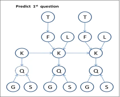
4.3 The process of entering evidence data - predict 1st question . . . 33

4.4 The process of entering evidence data - predict 2nd question . . . 34

4.5 The process of entering evidence data - predict 3rd question . . . 35

5.1 Individualization model. . . 42

5.2 Item diffficulty model. . . 44

A.1 Using bayesian knowledge tracing to generate data . . . 49

A.2 The trainig process of standard knowldege tracing. . . 50

A.3 The testing process of standard knowldege tracing. . . 50

A.4 Implementation of the CPT for KT-Forget model. . . 51

(9)

List of Tables

3.1 RMSE results of KT vs. correction models at item level . . . 20

3.2 RMSE results of KT vs. correction models at skill level . . . 20

3.3 RMSE results of KT vs. correction models at student level . . . 21

4.1 Knowledge Tracing residual analysis . . . 25

4.2 The CPT for knowledge node . . . 28

4.3 CPT of the forget node . . . 29

4.4 CPT of the slip node . . . 30

4.5 Residual and AUC results on standard KT (Cognitive Tutor) . . . 37

4.6 Residual and AUC results on KT-Forget (Cognitive Tutor) . . . 37

4.7 Summary and T-test on Standard-KT, KT-Forget and KT-Slip (Cog-nitive Tutor) . . . 38

(10)

Chapter 1

Background

1.1

Intelligent Tutoring Systems

Computer systems have been used for educational purposes since the early 1960s [10]. Intelligent Tutoring Systems (ITS) are such systems, which can effectively help students get better in learning. Since this thesis involved ITS, we will introduce it briefly in the following.

Intelligent tutoring systems have been shown to be highly effective in helping students learn better. For example, Shute et al. [28] claimed that students using an ITS for economics could perform equally well as students taking a traditional economics course, but required half as much time to cover the materials [4].

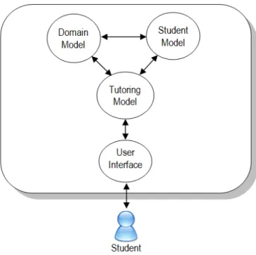
Although different ITSs may have different structures, e.g., in Corbett et al., 1997 [10]; Freedman et al., 2000 [15]; Massey et al., 1988 [18]; Woolf, 2008 [30], the basic structure of an ITS has four components: Student Model, Tutoring/Instructor Model, Domain Model, and User Interface, as presented in Figure 1.1.

(11)

1.1 Introduction

Figure 1.2: Main components of an Intelligent Tutoring System

3. Tutoring/Instructor Model(or Pedagogical Module): This module represents

teaching processes/strategies (examples and analogies). For example, information about when to review, when to present a new topic, and which topic to present is controlled by this pedagogical module. The student model is used as input to this module, so the pedagogical decisions reflect diﬀerent needs of each student (Beck et al., 1996).

4. User Interface(or Communication Module/Learning Environment): This

mod-ule presents the methods for interacting between the students and the systems, e.g. via graphical interfaces, animated agents, dialogs, screen layouts, etc. An important problem in this module is how the tasks (materials/learning objects) should be presented to the students in the most eﬀective way.

Indeed, Student Modeling in the ITSs has been taken into account over the years. One of the student modeling tasks is to trace the student’s knowledge, and thus stu-dent’s performance (student performance). According to Corbett & Anderson (1995), the student’s knowledge state is not fixed, but is assumed to be increasing. Thus, the authors have incorporated a Bayesian statistical model into the tutors for tracing the student knowledge, and eventually predicting student performance. This model was called Knowledge Tracing which now becomes the state-of-the-art method in student modeling and, as we will show in Chapter 4, the number of papers which have been

Figure 1.1: Main components of an Intelligent tutoring system

1.2

State of the Art

1.2.1

Bayesian Knowledge Tracing

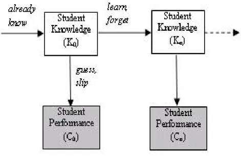
Student Modeling in ITS has been taken into account over the years. One of the student modeling tasks is to trace the student’s knowledge by using student’s perfor-mance. According to Corbett and Anderson (1995), the student’s knowledge state is not fixed, but is assumed to be increasing. Thus, the authors have incorporated a Bayesian statistical model into the tutors to trace the student knowledge, and even-tually predicting student performance. This model was called Bayesian Knowledge Tracing (KT) which now becomes the state-of-the-art method in student modeling. The KT is an Hidden Markov Model (HMM) [26] with a hidden node (student knowledge) and an observed node (student performance). It assumes that each

(12)

skill has 4 parameters; two knowledge parameters and two performance parameters

as shown in Figure 1.2. The two knowledge parameters are: initial (or prior)

knowledge and learn. The initial knowledge parameter is the probability that a

particular skill was known by the student before interacting with the tutor (e.g.

reading a text). The learn rate is the probability that a student will transition

between the unlearned state and the learned state after each learning opportunity

(or question). The two performance parameters are: guess and slip. The guess

is the probability that a student will guess the answer correctly even if the skill

associated with the question is in the unlearned state. The slip is the probability

that a student will answer incorrectly even if she is in the learned state.

These parameters dictate the model’s inferred probability that a student knows a skill given the student’s chronological sequence of incorrect and correct responses to questions that test that skill thus far. It is able to capture the temporal nature of data produced where student knowledge is changing over time. This concept of state change over time is very difficult to capture with classical machine learning approaches. KT provides both the ability to predict future student response values, as well as providing the different states of student knowledge. For this reason, KT provides insight that makes it useful beyond the scope of simple response prediction. Bayesian knowledge tracing has become the dominant method of modeling stu-dent knowledge for more than a decade. It is a variation on a model of learning first introduced by Atkinson in 1972 [2]. The goal of KT is to estimate the student knowledge from his or her observed actions. At each successive opportunity to apply a skill, KT updates its estimated probability that the student knows the skill, based on the skill-specific learning and performance parameters and the observed student performance (evidence).

(13)

$:DONWKURXJK([DPSOHRIPRGHOLQJ.QRZOHGJH7UDFLQJZLWK%1760

.QRZOHGJH7UDFLQJ.7LVDQHVWDEOLVKHGWHFKQLTXHIRUVWXGHQWPRGHOLQJDQGZDVILUVWXVHGLQWKH$&73URJUDPPLQJ/DQJXDJHV7XWRU7KHJRDORI.7LVWRHVWLPDWHWKH VWXGHQWNQRZOHGJHIURPKLVRUKHUREVHUYHGDFWLRQV$WHDFKVXFFHVVLYHRSSRUWXQLW\WRDSSO\DVNLOO.7XSGDWHVLWVHVWLPDWHGSUREDELOLW\WKDWWKHVWXGHQWNQRZVWKHVNLOO EDVHGRQWKHVNLOOVSHFLILFOHDUQLQJDQGSHUIRUPDQFHSDUDPHWHUVDQGWKHREVHUYHGVWXGHQWSHUIRUPDQFHHYLGHQFH5H\HVKRZHGWKDW.7LVVSHFLDOFDVHRID'%1ZKLFK DVVXPHVSDUDPHWHUVGRQRWFKDQJHDFURVVWLPHVOLFHV0RUHVSHFLILFDOO\WKHFRQGLWLRQDOLQGHSHQGHQFHJUDSKRI.7FDQEHGUDZQDVWKHIROORZLQJ)LJXUH:HUHQDPHWKH RULJLQDO.7YDULDEOHV/DQGWDVDOUHDG\NQRZDQGOHDUQIRUFRQVLVWHQWQDPLQJZLWKRWKHUVHFWLRQV ,QWKHIROORZLQJVHFWLRQVZHZLOOEULHIO\JRRYHUWKHIRUPDWRIWKHLQSXWDQGRXWSXWILOHV7KHUHDUHDGGLWLRQDOGHWDLOVLQWKHILOH5($'0(W[WDWWKHWRSOHYHOGLUHFWRU\LQWKH SDFNDJH

SURSHUW\B[PO

"[POYHUVLRQ "! SURSHUW\! LQSXW! HYLGHQFHBWUDLQ!HYLGHQFHWUDLQ[OVHYLGHQFHBWUDLQ! HYLGHQFHBWHVW!HYLGHQFHWHVW[OVHYLGHQFHBWHVW! LQSXW! LQIHUHQFH!IDVWLQIHUHQFH! RXWSXW! SDUDPBWDEOH!SDUDPBWDEOH[OVSDUDPBWDEOH! LQIHUHQFHBUHVXOW!LQIHUHQFHBUHVXOW[OVLQIHUHQFHBUHVXOW! LQIHUHQFHBUHVXOWBKHDGHU!LQIHUHQFHBUHVXOWBKHDGHU[OVLQIHUHQFHBUHVXOWBKHDGHU! LQIHUHQFHBLVBSULRU!\HVLQIHUHQFHBLVBSULRU! ORJ!ORJW[WORJ! RXWSXW! VWUXFWXUH! YDU!) 7 YDU! QRGHV! QRGH! LG!LG! QDPH!NQRZOHGJHQDPH! W\SH!GLVFUHWHW\SH! YDOXHV!YDOXHV! ODWHQW!\HVODWHQW! ILHOG!NQRZOHGJHILHOG! ZLWKLQ! WUDQVLWLRQ!DVUBDFFHSWWUDQVLWLRQ! ZLWKLQ! EHWZHHQ! WUDQVLWLRQ!NQRZOHGJHWUDQVLWLRQ! EHWZHHQ! QRGH! QRGH! LG!LG! QDPH!DVUBDFFHSWQDPH! W\SH!GLVFUHWHW\SH! YDOXHV!YDOXHV! ODWHQW!QRODWHQW! ILHOG!DVUBDFFHSWILHOG! ZLWKLQ!ZLWKLQ! EHWZHHQ!EHWZHHQ! QRGH! QRGHV!

Figure 1.2: A description of Bayesian Knowledge Tracing

According to Corbett and Anderson (1995), the following equation is used in knowledge tracing to update the estimate of the student’s knowledge state:

p(Ln) =p(Ln−1|evidence) + (1−p(Ln−1|evidence))∗p(T) (1.1)

The probability of a skill in the learned state following the nthopportunity to apply

the skill, p(Ln), is the sum of two probabilities: (1) the posterior probability that

the skill is already in the learned state contingent on the evidence (whether or not

the nth action is correct) and (2) the probability that a skill make transition to the

learned state if it is not already there. Bayesian inference scheme is used here to

estimate the posterior probability p(Ln1|evidence). Following Atkinson (1972) [2].

the probability of p(T) of the transition from unlearned to learned state during

procedural practice, which is independent of whether the student applied the skill

(14)

correctly or incorrectly.

Corbett and Anderson introduced this method to the intelligent tutoring field in 1995 [9]. It is currently employed by the Cognitive Tutor [1], used by hundreds of thousands of students, and many other intelligent tutoring systems to predict student performance and determine when a student has mastered a particular skill.

1.2.2

Limitations

Despite the proven utility of the knowledge tracing approach, it does have some critical limitations.

For example, one limitation is that the four parameters of KT are learned for each skill regardless of the individual students learning that skill. This means that the KT does not take into account “individualization”. For example, it does not

support students having different prior knowledge or differentlearn rates.

Pardos & Heffernan (2010) [20], proposed the KT-PPS (Prior Per Student ) model which individualized the prior knowledge parameter and had successfully tackled this limitation of the KT. The difference between the KT-PPS and the stan-dard knowledge tracing model is the ability to represent a different prior knowledge

parameter for each student, therefore, the prior knowledge parameter denoted as

P(L0) in the learning Parameters is changed to P(L0[s]) for an individual student

s. The P(L0[s]) is then used for the knowledge tracing phase of that student. A

short description of the KT-PPS is presented later in Chapter 6.

Another limitation is that KT has no underlying mechanism for memory

de-cay [16] represented in the model. There is a f orget parameter presented in KT

model; however, in most KT implementations this is fixed at 0, which means that there is no forgetting happening. Thus, even over significant periods of non-practice,

(15)

when some forgetting would inevitably occur, the student model assumes that the student’s knowledge state remains stable across periods of non-use, leaving all prior learning completely intact. This limits the utility of traditional student modeling approaches entirely to estimates of current proficiency (mastery). They have no capacity to predict what future readiness will be at specific points in time.

In all, we can see that numerous past researchers have shown that KT has its limitations. Many modifications to the KT model that improved the prediction accuracy of student performance have been proposed and evaluated, however unfor-tunately many of these modifications are often based on a combination of intuition and experience in the domain. This method of model improvement can be difficult for researchers without high-level of domain experience and the best improvements to the model could be unintuitive ones.

Furthermore, the knowledge tracing model can be computationally expensive [3][27]. Model fitting procedures, which are used to train KT, can take hours or days to run on very large datasets.

(16)

Chapter 2

Introduction

2.1

Motivation

Predicting student performance is an important part of the student modeling task in ITS [11]. This problem has attracted not only the ITS and the Educational Data Mining communities but also the Machine Learning and Data Mining communities. It was selected as a challenge task for the KDD Challenge 2010 at the KDD 2010 Conference and a following workshop on Knowledge Discovery in Educational Data was also organized at the KDD 2011 Conference.

Specifically, predicting student performance is the task where we would like to know how the students learn (e.g., generally or narrowly), how quickly or slowly they adapt to new problems [17] or if it is possible to infer the knowledge requirements to solve the problems directly from student performance data [9] [14]. Eventually, we would like to know whether the students perform the tasks (problems/exercises) correctly (or with some levels of certainty) when interacting with the tutoring sys-tem.

(17)

Accurately predicting student performance is thus a very important and valuable task. By predicting their performance on the tutoring system we can understand how the students learned, and the more we understand the students internal knowledge state the more we can assist them by providing them with appropriate feedback, and help them improve while using the ITS.

As discussed in Cen (2009), an improved model for predicting student perfor-mance could save millions of hours of students’ time and effort in learning algebra. In that time, students could move to other specific fields of their study or doing other things they enjoy. Moreover, many universities are extremely focused on as-sessment. Thus, the pressure on teaching and learning for examinations leads to a significant amount of time spent for preparing and taking standardized tests. Any move away from standardized and non-personalized tests holds promise for increas-ing deep learnincreas-ing [14]. From an educational data minincreas-ing point of view, an accurate and reliable model in predicting student knowledge may replace some current stan-dardized tests and thus, reducing the pressure, time, as well as effort on teaching and learning for examinations [14]. Furthermore, by predicting student knowledge the instructors could also help the student study better by providing early feedback.

2.2

Problem Definition

As we mentioned in the previous chapter, the standard Bayesian Knowledge Tracing has many critical limitations. One specific limitation is that KT has no underlying mechanism for “memory decay” represented in the model. The forget parameter in the model is fixed at 0, which means that once a skill is in the learned state there is no reverse back to unlearned state. Also, the Bayesian Knowledge Tracing

(18)

model can often be computationally expensive when the datasets are large, so it is important for us to determine that the intuitive modifications to the model are inexpensive. In summary:

Problem 1: Modeling based on intuition can be unintuitive and the evaluation

of the student model can often be expensive.

Problem 2: A basic problem arises when students are working on a skill across

several days. The standard KT model assumes no probability of forgetting. which means there is no memory decay factor in the model.

Problem 3: Poor performance on a another day may also suggest that students

may not actually be “forgetting” but instead, they might just be “slipping.”

2.3

Goals Achieved

The goal of this research work is to improve the accuracy of student performance prediction by incorporating the memory decay factor which the standard Bayesian Knowledge Tracing ignored. We design, implement and evaluate a model that takes this factor into consideration.

We also propose a completely data driven approach to model improvement. This alternative allows researchers to evaluate which aspects of a model are most likely to result in model performance improvements based purely on the dataset features (e.g., ITS computer logs). As shown in Figure 2.1. To summarize:

• We show assumptions made in knowledge tracing model, that student don’t

forget, is false. While this might not be terribly surprising, we identify a particular situation in which the standard KT model has systematic errors in predicting student performance, which is on “new day” responses. Here “new

(19)

3.2 Data Mapping for Collaborative Filtering

the ASSISTments data set has the structure

Assignment

⊇

Assistment

⊇

P roblem

From this structure, we can easily recognize that each Assignment has one or many

ASSISTments, and each ASSISTment consists of one or more problems.

Moreover, instead of naming “knowledge component” as in the KDD Cup 2010 data,

the ASSISTments calls it the

skill. Target of the prediction task is also the

correct first

attempt

information which encodes whether the student successfully completed the

given

problem

on the first attempt.

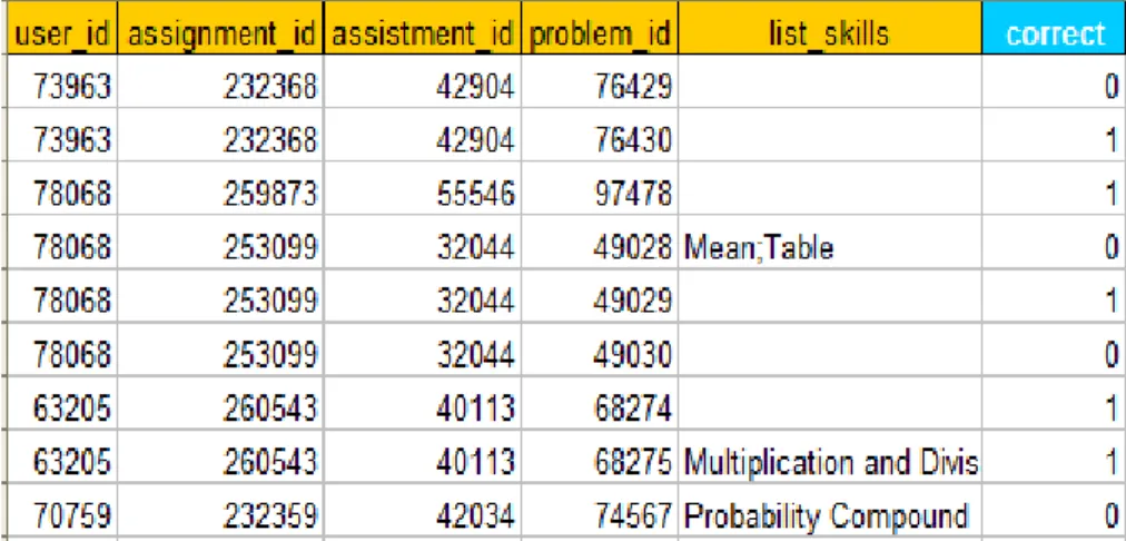
A snapshot of this data set, which includes the attributes that we have used for

experiments, is presented in Figure 3.2. For more information, please see Feng

et al.

(2009) and descriptions from the ASSISTments Platform

1

.

Figure 3.2: A snapshot of the ASSISTments data set

Except the other attributes in these data sets which we have not used yet, the only

diﬀerence between the KDD Cup 2010 and the ASSISTments data is just the naming

convention (please note that in the KDD Cup 2010 data, the task is to predict a single

step while the task is to predict a single problem in the ASSISTments data).

Therefore, for easiness in naming convention reason, we assume that these data

share some similarities (although they come from diﬀerent platforms and may aim at

diﬀerent purposes). Using our notations, we denote them in a uniform way, as presented

in Table 3.2

3.2 Data Mapping for Collaborative Filtering

In traditional recommender system settings, it is unambiguous how the available

in-formation is mapped to users, items, and ratings, respectively. At least for all major

1

http://teacherwiki.assistment.org

21

Figure 2.1: An example of the ASSISTments data set

day” means the next item is not done on the same day with the previous item.

• We present a model that takes this phenomenon into account, which does a

reliably better job of fitting student data in some datasets than the standard KT. This is significant as KT has proved itself to be a very effective model, which is difficult to improve upon. It is also noteworthy that KT is easily interpretable and it is therefore beneficial to be able to have a new model that fits easily into the Bayesian framework and inherits this interpretability. Our contribution is that we have demonstrated a method that takes “time” into account and improves modeling performance.

• We describ a methodology for identifying areas within a model that can be

improved upon. The residual corrections of our different features gave a strong indication that time between responses would be of significant benefit to the knowledge tracing model.

(20)

account as a modification will lead to a significant improvement to the standard Bayesian Knowledge Tracing model. The model propose in Chapter 4 of this thesis is good proof of the feasibility of this method.

The contributions of this thesis were published in several international confer-ences and workshops

2.4

Chapter Overview

The document is organized as follows:

• In Chapter 1 we briefly introduced the background of Intelligent Tutoring

System and the state-of-the-art model Bayesian Knowledge Tracing and its limitations.

• In Chapter 2 we identified the importance and the value of accurately

predict-ing student performance, defined the tasks of this research work and described the goals we have achieved.

• Chapter 3 presents the solution for the first proposed problem. We describe

datasets that are used for experiments and used the dataset features (computed from computer log) to identify useful feature for student model improvement. This work is published in Proceedings of the 25th International FLAIRS Con-ference.

– Y. Qiu, Z. Pardos and N. Heffernan. Towards Data Driven Model

Im-provements in 25th International FLAIRS Conference. Marco Island. 2012.

(21)

• Chapter 4 proposes a model that incorporates the f orget factor, We presente how our models work and how to use them to make prediction. This work in published n Proceedings of the 4th International Conference on Educational Data Mining, 2011.

– Y. Qiu, Y. Qi, H Lu, Z. Pardos and N. Heffernan. Does Time Matter?

Modeling the Effect of Time with Bayesian Knowledge Tracing. in Fourth International Conference on Educational Data Mining. 2011. Pages 139-148.

• Chapter 5 summarizes some of the related work in student performance

pre-diction improvement.

• Chapter 6 puts all the proposed methods into context for conclusion. We also

(22)

Chapter 3

Data Driven Approach to Student

Model Improvements

In this chapter, we propose a completely data driven approach to model improve-ment. This alternative allows for researchers to evaluate which aspects of a model are most likely to result in model performance improvement. Our results suggest a variety of different improvements could be add to knowledge tracing, many of which have not been explored.

3.1

Dataset

We analyzed the KT model with a dataset from a real world tutor called the Cog-nitive Tutor [1]. Our CogCog-nitive Tutor dataset comes from the 2006-2007 “Bridge to Algebra” system. This data was provided as a development dataset in the 2010 KDD Cup competition [21].

(23)

cur-riculum, which is split into sections. The problems consist of many steps (associated with skills) that students must answer to go to the next problem. The Cognitive Tutor uses the Knowledge Tracing model to determine when a student has mas-tered a skill. A problem in the tutor can also consist from questions of various skills. However, once a student has mastered a skill, as determined by KT, the student no longer needs to answer questions of that skill within a problem. When a student mastered all the skills in their current section they are allowed to move on to the next section. The time for students using this system is determined by their teachers.

3.2

Selected Attributes

The original Cognitive Tutor dataset consists many attributes such as student ID; step name, problem name; sub-skill name; step start time; hints and many more. In this chapter our primary goal is to discover how time information would impact model improvement.

To make the dataset more interpretable, five features were computed from the original dataset most related to student performance time to test its individual impact on model improvement. The chosen features are listed below:

• Time interval between responses

• Count of the number of days spent trying to master a skill

• Opportunity count (number of steps answered in a skill)

(24)

• Percent correct of a skill done by multiple students

The specific description of the features are as below:

• The “time interval” between responses was separated into four bins: 1 means

the items were done on the same day; 2 means the time interval between the consecutive items is one day; 3 means the time interval is within a week; and 4 means the time interval between consecutive responses is more than a week.

• The features of “percent correctness of student” and “percent correctness of

skill” were calculated base on the number of correct responses for one student and for that skill, it is a fraction between 0 and 1.

• The “day count” feature was calculated based on the number of days the

student worked per skill.

• As for “opportunity count”, it represents how many responses a student made

per skill.

The original dataset was divided by sub-skills. Each sub-skill such as “identify

number as common multiple”,“list consecutive multiple of a number”and“calculate

the product of two numbers” was counted as a skill in this analysis. Each skill

individually is counted as a dataset. Here, eleven skills were randomly chosen from the pool of math skills that the original dataset provided for analysis, which exclude

the action steps such as“press Enter”that do not represents math skills. The skills

(25)

3.3

Methodology

A two-fold cross-validation was done in order to acquire the KT model prediction on the datasets. The two-fold cross-validation involved randomly splitting each dataset into two bins, one for training and one for testing. A KT model was trained for each skill. The training phase involved learning the parameters of each model from the training set data. The parameter learning was accomplished by using the Expectation Maximization (EM) algorithm [7]. In this work EM attempts to find the maximum log likelihood fit to the data and stops its search when either the max number of iterations specified has been reached or the log likelihood improvement is smaller than a specified threshold.

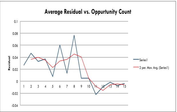
Since we wanted to learn more about exactly how KT was performing we com-bined all the prediction results together in order to track residuals on a per-opportunity basis. Figure 3.1 show the graph for the first 15 student responses. It should be noted that the majority of our student response sequences are about 10 responses long. The behavior of the graphs from 11-15 is based on fewer data points than the rest of the graph. The residual graph showed that KT is under-predicting early in the response sequence. In Wang et al. [29], their intuition for this phenomenon is that KT takes too long to assess that a student knows a skill and once it believes a student knows a skill, KT over-predicts correctness late into a student’s response sequence. Essentially the authors point out that KT has systemic patterns of errors. We believe these errors can be corrected for by looking to unutilized features of the data.

With Figure 3.1 we were able to convince ourselves that some simple correction could exist that could smoothen the residual curve in order to improve the model.

(26)

-0.04 -0.02 0 0.02 0.04 0.06 0.08 0.1 1 2 3 4 5 6 7 8 9 10 11 12 13 14 15 R es id u a l

Average Residual vs. Oppurtunity Count

Series1

2 per. Mov. Avg. (Series1)

Figure 3.1: Individualization model.

In this paper we conducted three experiments to evaluate the five attributes of the dataset discussed above.

3.3.1

Experiment 1: Item Level

In the first experiment, the selected 11 skills were combined together to make a one large dataset, each row representing a student response to a given problem and are all treated equally regardless of which skill it was from. A five-fold cross-validation was used to make predictions on the dataset, which means randomly splitting the dataset into five bins at the response level.

As we want to know which attributes of the dataset can could lead to an improve-ment of the KT model,. An regression analysis was conducted for each attribute.

(27)

Regression analysis is used to understand which among the independent variables are related to the dependent variable. The regression function is shown below.

In this function the unknown variable is denoted as β, the dependent variable is

denoted as Y and the independent variable is denoted as X.

Y _≈f(X, β) (3.1)

All analysis takes the residual result of the KT model as the dependent variable and the selected attributes of the dataset are treated as the single independent variable of each analysis. After a linear regression function was trained for each feature, the estimated value of the unknown variable was treated as a correction to the prediction of the KT model. Therefore we gain the corrected prediction

of that attribute. By doing this we are able to predict patterns in KT’s error

(residual) based on various dataset features (independent variable). If the error can be predicted with high accuracy then this tells us that the KT model can benefit from inclusion of that variable information.

3.3.2

Experiment 2: Skill Level

The second experiment was done at the skill level. Similar to Experiment 1 a five-fold cross-validation was also used to make prediction on the dataset. There are five rounds of training and testing where at each round a different bin served as the test set, and the data from the remaining four bins served as the training set. Note that the skills in the training set will not appear in the testing set in order to avoid over-fitting. The cross-validation approach has more reliable statistical properties than simply separating the data in to a single training and testing set and should

(28)

provide added confidence in the results.

The regression analysis was also conducted similar to Experiment 1 and the new model prediction was corrected based on the given attributes. Because this

correction is done at the skill level the analysis for the attributes “percent correct

by skill” was omitted here.

3.3.3

Experiment 3: Student Level

The third experiment was done at the student level. Similar to Experiment 1 and 2, a five-fold cross-validation was also used to make prediction on the dataset. There will still be five rounds of training and testing where at each round a different bin served as the test set, and the data from the remaining four bins served as the training set. Note that the student in the training set will not appear in the testing set in order to avoid over fitting.

The regression analysis was also conducted similar to experiment 1 and 2. The new model prediction was corrected based on the given attributes, also here in

experiment 3 the attribute “percent correct by student” was also omitted because

the correction is done at the student level.

3.4

Experiment Results

Predictions made by each model were tabulated and the accuracy was evaluated in terms of root-mean-square error (RMSE). RMSE is a frequently used measure of the differences between values predicted by a model or an estimator and the values actually observed from the thing being modeled or estimated. Here we use the Knowledge Tracing model prediction residual as the observed value. Therefore

(29)

the correction is apply to the residual it would minimize it’s distance to the ground truth.

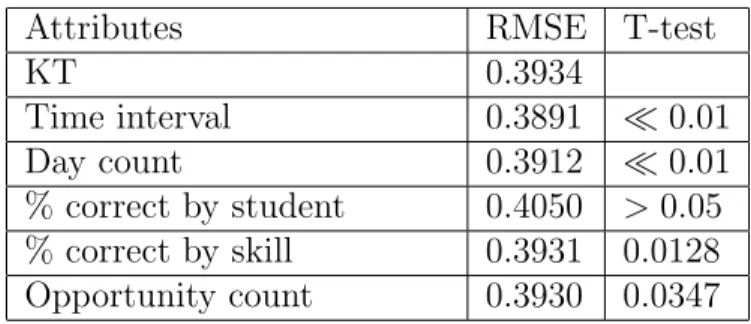
The cross-validated model prediction results for Experiment 1 are shown in Ta-ble 3.1; the cross-validated model prediction results for Experiment 2 are shown in Table 3.2 and the cross-validated model prediction results for Experiment 1 are shown in Table 3.3. The p-values of paired t-test comparing the correction models and the standard KT model are included in addition to the RMSE for each model in each table.

Table 3.1: RMSE results of KT vs. correction models at item level

Attributes RMSE T-test

KT 0.3934 Time interval 0.3891 0.01 Day count 0.3912 0.01 % correct by student 0.4050 >0.05 % correct by skill 0.3931 0.0128 Opportunity count 0.3930 0.0347

Table 3.2: RMSE results of KT vs. correction models at skill level

KT 0.3934

Time interval 0.3898 0.01

Day count 0.3928 0.2639

% correct by student 0.4047 >0.05

Opportunity count 0.3937 0.0686

The results from evaluating the models with the Cognitive Tutor datasets are strongly in favor of the time interval correction model in all three experiments, with

(30)

Table 3.3: RMSE results of KT vs. correction models at student level

KT 0.3934

Time interval 0.3892 0.05

Day count 0.3913 0.05

% correct by skill 0.3929 0.05

Opportunity count 0.3932 0.2451

KT was 0.3934while the average RMSE for the time interval correction model were

0.3892, 0.3898 and 0.3892. These differences were all statistically significant with

p= 1.92E₋10, p= 1.27E₋08 and p= 2.61E₋10 respectively, using a two tailed

paired t-test.

As for the other correction models the three experiments all agree that the

“percent correct by student” features is not useful for improving the KT model and

“opportunity count” is also not a very good correction model. We can assume that

it is not very likely to see a large improvement if this feature is considered as the correction to the KT model. According to Table 3.1 and Table 3.3, the day count

correction model’s average RMSE were 0.3912 and 0.3892 which are both better

than the KT RMSE 0.3934 and the difference are all statistically significant with

p = 1.05E₋06 and p = 4.74E₋06, respectfully. Howerver the evaluation at the

skill level seems not to agree to the other evaluations, even though the error is still smaller but it is not significantly reliable.

From the experiments above, we assume that taking “time interval” feature

into account as a modification will lead to a significant improvement to the stan-dard Knowledge Tracing model. The model proposed in the next chapter [25] is a demonstration of the feasibility of this method. Currently with the results from

(31)

this chapter we can eliminate the work of trying to improve student assessment with

this dataset by using the attribute of“percent correct by students”but the other two

attributes “percent correct by skill” and “day count” still need further evaluation.

In particularly the “day count” feature seems to have a good potential to improve

(32)

Chapter 4

Modeling the Effect of Time

When using the standard Knowledge Tracing (KT) model, it is assumed that the students’ probability of making the transition from the unlearned to the learned state is constant opportunities (or questions). Many researchers have proposed extensions to Bayesian Knowledge Tracing [8], however none have tried to incorporate into the model how much time has elapsed between opportunities. They all assume that student performance a minute later is the same as the next day. Nonetheless, ever since Ebbinghaus inaugurated the scientific study of memory [12], researchers have examined the manner in which memory performance declines with time or intervening events [24].

4.1

Problem Statement

In the real world, coming into class on a new day may result in a student forgetting the material or a higher probability of them slipping. By taking this real world fact into consideration, in this chapter we look into how KT performs on each new day’s

(33)

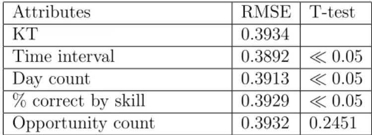
responses. We define a new day’s response as a response that occurred on a later calendar date than the student’s previous response to a question of the same skill. We found that KT’s new day error is far higher than same day error. A residual analysis showed that KT was largely over-predicting student performance on each new day response. The residual analysis is shown in Table 4.1.

Based on the residual result Table 4.1 and Fig 4.1, we made two hypotheses to explain this phenomenon; 1) that students may forget between days and 2) that stu-dents may slip when answering the first question on a new day. The slip hypothesis only affects the model’s prediction of new day events while the forget hypothesis could affect prediction of subsequent responses since it hypothesizes a change in the latent knowledge. We developed two new models based on knowledge tracing: a KT-Forget Model and a KT-Slip Model, where a new day variable is taken into account to affect either students’ knowledge or performance. To implement this, we introduced a new split-parameter KT model, which allowed us to, for instance, learn a different forget parameter for new day opportunities than for same day but learn only a single learn rate parameter for each.

In the following sections we will describe the model design in. Section 4.2 presents the model design that incorporates the time concept. The evaluations of the pro-posed models are the focus of Section 4.3 and summarized in Section 4.4. To con-clude, we identify and discuss open areas of research for future work in Section 4.5.

(34)

Table 4.1: Knowledge Tracing residual analysis

Problem Set Residue Same Day Residue New Day

1 0.039803 -0.363268 2 -0.026765 -0.110578 3 0.088299 -0.076079 4 -0.014643 -0.117302 5 -0.003538 -0.062383 6 0.018866 -0.160024 7 0.009965 -0.109267 8 -0.049156 -0.169034 9 0.023225 0.032221 10 -0.029405 -0.010356 11 0.013791 -0.275969 12 0.082811 -0.054692 Average 0.012771 -0.123060 -0.4 -0.35 -0.3 -0.25 -0.2 -0.15 -0.1 -0.05 0 0.05 0.1 0.15 1 2 3 4 5 6 7 8 9 10 11 12 R es id u a l Problem Set Same Day Residual New Day Residual

(35)

4.2

Time Model Design

When using the Bayesian Knowledge Tracing model, it is assumed that the student’s probability of making the transition from the unlearned to the learned state is not changing across opportunities, while in the real world there might be a time elapse since students’ last opportunity. This fact assumes that there is a great possibility that a student’s forgetting rate is not zero. The standard KT model assumes no probability of forgetting. Prior work has modeled forgetting between sessions in a lab but did not allow within-day learning to occur [22]. Alternatively, poor performance

on a new day may also suggest that students may not actually be “forgetting” but

instead, they might just be “slipping” We used Bayesian networks and Expectation

Maximization to detect whether time had any influence on the forget parameter and the slip parameter of the KT model [19]. The model with the better predictive accuracy will indicate the better cognitive explanation of the data.

4.2.1

Split - KT Model Design

In order to determine the validity of this method, we represent the above two hy-pothesis in the Bayesian Knowledge Tracing model by introducing a novel modifi-cation to the model that allows us to fit a same day and new day parameter for one parameter in a Conditional Probability Table (CPT) while keeping the other parameter in the CPT constant. In Knowledge Tracing; learn and forget share a CPT and guess and slip share a CPT. As shown below, the difference between

split-KT and the standard-split-KT is the ability to separate the f orget, learn, guess, and

slip parameters individually. The equivalence between these two KT models was

(36)

without new day data, and confirming that the learned parameters and predictions were the same. We also compared the computational run time of the split-KT and standard-KT. We tested on one of the dataset from ASSISTment which contained 527 data points and calculated the EM parameter learning time of the two mod-els. It took approximately 70 seconds for the standard-KT to learn the parameters and 102 seconds for Split-KT, which equates to a penalty of about 50% to run the Split-KT model. Both models resulted in the same learned parameters.

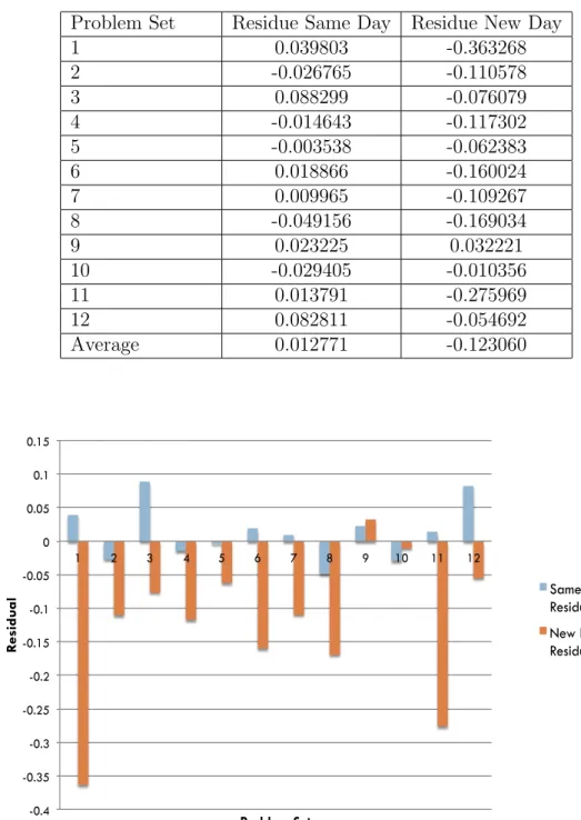
The individualization of the four parameters were achieved by adding a forget node and a learn node to the knowledge node, as well as adding a guess node and slip node to the question node. Therefore, the knowledge nodes and question nodes are conditioned upon the four new nodes. The CPT for knowledge node is given in Table 4.2. The CPT for the question node is also of this form, the only

difference is changing thelearnandf orgetparameters toguessandslipparameters

and changing the previous and current knowledge to previous and current student performance. The question and knowledge CPTs are fixed and essentially serve as logic gates. The guess, slip, learn and forget node CPTs contain the continuous probabilities that are familiar to the standard KT model. Taking the first row as an example, knowing that the students do not have previous knowledge of the skill

(Knowledge previous=F), and they neither learn nor forget (learn=F, f orget=

F), then we can infer the probability that students have the current knowledge is 0

(P(Knowledge current=T) = 0).

This model can easily let us set individualized learn rates, forget rates, guess

rates and slip rates. This way we are able to fix the learn parameter and guess

parameter in order to investigate how new day instances would affect the f orget

(37)

Table 4.2: The CPT for knowledge node

Learn Forget Knowledge previous P( Knowledge current=T) = 0

F F F 0 T F F 1 F T F 0 T T F 1 F F T 1 T F T 1 F T T 0 T T T 0

4.2.2

KT - Forget Model

In this section we focus on one of the hypotheses: How would the new day instance affect the forget parameter. We think that it is highly possible that students could be forgetting the previously learned knowledge when there are several days interval between the practices on the ITS.

The model we used to test our hypotheses is a new model built based on the Split-KT model discussed in the previous section. By adding a time node to the Split-KT model we are able to easily specify which parameters of the model should be affected by a new day. The new day node is fixed with a prior probability of 0.2, which is the overall proportion of the new day instances in the dataset. The topology of the KT-Forget model is shown in Figure 4.2.The forget node is only conditioned on the added new time node, so there is only one new parameter

“f orget n” introduced in this KT-Forget model and represents the forget rate on

a new day. We use “f orget s” to denote the forget rate on a same day, which we

set to be 0 just as the forget parameter in the original Knowledge Tracing model implying that there is no forgetting between opportunities in the same day.

(38)

Table 4.3: CPT of the forget node

New Day P(Forget=T)

F 0

T f orget n

The CPT for the forget node in this model is shown in Table 4.3. This table says

that when a new day response occurs, N ew Day=T, the probability that student

forget knowledge is f orget n, P(F orget=T _|N ew Day =T) and is 0, otherwise.

4.2.3

KT - Slip Model

An alternate hypothesis is that while students might be performing on the ITS across several days, they are not forgetting the previously learned material. Rather, the students are just making a mistake on the first question of the day (rustiness effect) after which they no longer slip at a higher than usual rate. So the low accuracy on

first attempt on a new day might not be captured in the f orgetparameter. It could

be that they just slipped and answered wrong. This explanation makes it necessary

for us to look into the slip parameter.

The KT-Slip model is similar to the KT-Forget model and can be represented simply by connecting the time node to the slip node instead of connecting to the forget node as in the Forget model. The Slip model allows us to model the different slip rates of the new days and the same days. The Slip model is shown in Figure 4.2 in the bottom box.

Since the slip node is only conditioned on the added new time node, there is

also one new parameter slip n introduced in this KT-slip model, which represents

(39)

Table 4.4: CPT of the slip node

New Day P(slip = T)

F slip s

T slip n

which is shown in Table 4.4. This table says that when a new day response occurs,

N ew Day = T, the probability of slipping is slip n, P(slip= T _| N ew Day = T)

and is slip s, otherwise.

4.3

Topology of the Models

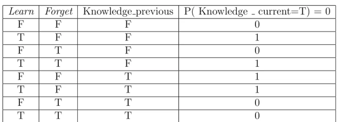
The Split-KT model’s topology is shown together with KT-Slip and KT-Forget in Figure 4.2 Boxes in the figure denote the portions of the figure that are used in each model. While all models are shown in this figure so the relationship between them can be seen. When the models are run, they are run separately as a separate topology and not one big model.

4.4

Model Performance Evaluations

To evaluate the performance of the KT-Forget and the KT-Slip models. We used a Cognitive Tutor dataset and ASSISTments dataset to test the real world util-ity of these models by comparing their predictive performance with the standard KT model. For each problem set, which represents a specific skill we trained stan-dard KT, KT-Forget and KT-Slip models to make predictions on all the question responses of each student. Then the residuals and area under curve (AUC) is

(40)

cal-K

Q

K

Q

F

L

F

L

S

G

Split-‐KT Model Parameters

P(!"): Probability of initial Knowledge P(F): Probability of forget P(L): Probability of learn P(G): Probability of guess P(S): Probability of slip

Node Representation

K: Knowledge node L: Learn node Q: Question node G: Guess node F: forget node S: Slip node T: Time node

The Proposed Time Model

T

Forget Model Parameters P(!"): Probability of initial Knowledge P(#$): Probability of forget on same day P(#%): Probability of forget on new day P(L): Probability of learn

P(G): Probability of guess P(S): Probability of slip

P(T): Probability of new day instance Slip Model Parameters

P(!"): Probability of initial Knowledge P(#): Probability of forget P(L): Probability of learn P(G): Probability of guess P(#&): Probability of slip on same day P(#%): Probability of slip on new day P(T): Probability of new day instance Regular-‐KT Model

Figure 4.2: The topology of the models - Split-KT, KT-Forget, KT-Slip well as overall events to analyze the three models’ performance. The residual is the mean of the actual performance subtracted by the predicted performance. AUC is a robust accuracy measure where a score of 0.50 represents a model that is only as good as chance and 1.0 represents a perfectly predicting model.

The analysis method consisted of two steps: run Expectation Maximization to fit the parameters on the training set for each model, and apply the trained parameters to the test sets to predict the student performance on each question

(41)

4.4.1

Datasets for Prediction

One of the datasets comes from the Cognitive Tutor System called Bridge to Algebra and is from the 2006-2007 school year. This was one of the smaller, development datasets made public as part of the 2010 Knowledge Discover and Data mining competition [21]. In this tutor, students answer algebra problems from their math curriculum which is split into sections. The problems consist of many steps that the students must answer to go to the next problem. A student no longer needs to answer steps of a given skill when the Cognitive Tutor’s Knowledge Tracing model believes the student knows the skill with probability 0.95 or greater. When a student has mastered all the skills in their current section they are allowed to move on to the next. The time for students using this system is determined by teachers. Twelve skills were chosen at random from this dataset for analysis (excluding skills such as “press enter” which do not represent math skills). There was an average of 122 student per skill in this dataset.

Another dataset is collected from ASSISTments Platform’s Skill Builder problem sets. The ASSISTments Platform is an educational research platform known for its e-learning [13] that provides web-based math tutoring to 8th-10th grade students. Unlike the Cognitive Tutor System, students are forced to leave the tutor after 10 questions have been finished in one day and will come back to the tutor in a new day. If a student answers three questions correct in a row, they are considered as master the problem set. The help function this tutor provides is consists of a series of questions that break a problem into sub steps. A student can also request a hint, but requesting a hint will mark the student as getting the step wrong in the system. Only answers to the original questions are considered. The largest twelve

(42)

Skill Builder datasets were selected from the ASSISTments Platform. There was an average of 1,200 students per problem set in this dataset. The highest student count problem sets were selected here because new day events are far sparser in ASSISTments skill problem sets than the Cognitive Tutor skill problem sets.

The twelve datasets from each tutor were randomly divided into two equal parts by student, one part was used as the training set, the other as the testing set.

4.4.2

Prediciton Procedure

Parameters were learned for each skill problem set individually. The parameters

were unbounded and initial parameters were set to a guess of 0.14, slip of 0.09,

prior of 0.50 and learnof 0.14.

K Q K K Q Q F L F L S S S G G G Predict 1st _question T T

(43)

K

Q

K

Q

F

L

F

L

S

G

Predict 2nd _question

T

(44)

K Q K K F L F L S S S G G G Predict 3rd _question T T Q Q

Figure 4.5: The process of entering evidence data - predict 3rd question

These initial values were the average parameter values across all skills in prior modeling work conducted on the ASSISTments tutor [22]. Since both tutors, AS-SISTments and the Cognitive Tutor cover the similar domains, algebra, and that they are within plausible parameter range we use the above parameters for both datasets.

For parameter learning, the new day observation (0 or 1) was presented as ev-idence in addition to the student responses. After training, the time and actual response values were given to the model as evidence for our new models to do the prediction (for standard KT, only actual responses were given as evidence) one stu-dent at a time. In order to predict every response of each stustu-dent in the test set, the student data for prediction was presented to the network in the following fashion: for predicting the first question, no evidence was entered; for the second question, the new day information for that question and the actual response of first question

(45)

were entered as evidence; for the third question, the first two new day information and responses information were entered as evidence. Apply this procedure until the prediction of the last question. This predicting process is shown in Figure 4.3, Figure 4.4 and Figure 4.5, the “Dotted Outline Node” denotes the prediction node and the “Shaded Nodes” denote the evidence for the prediction node. By applying this prediction process, the probability of student answering each question correctly was computed and saved.

The results summary of all three models across problem sets as well as the results of pairwise t-test is shown in Table 4.7.

4.4.3

Prediction Result Analysis

The prediction performance of the three models were calculated in terms of residuals and AUC values between predictions and actual responses on same day events, new day events as well as overall events of the whole problem set. The model with higher AUC values for a problem set was deemed to be the more accurate predictor of that problem set. In addition, a two-tailed paired t-test was calculated between standard KT and KT-Forget and standard KT and KT-Slip. We first applied this to the datasets collected from Cognitive Tutor. The specific results of each problem sets are shown below for standard KT (Table 4.5) and KT-Forget (Table 4.6).

From the above results, generally, we can see that the new KT-Forget model performed better on both the residuals and AUC compared to the standard KT model. Conversely, the KT-Slip model performed worse than we expected. The specific evaluation of the two new models is shown in Table 4.7 and Table 4.8 . For the KT-Forget model, improved results were obtained both on residuals and AUC.

(46)

Table 4.5: Residual and AUC results on standard KT (Cognitive Tutor)

standard KT Residual AUC

Problem Set Overall Same Day New Day Overall Same Day New Day

1 -0.0263 0.0398 -0.3633 0.5952 0.6570 0.4972 2 -0.0390 -0.0268 -0.1106 0.7588 0.7434 0.8669 3 0.0623 0.0883 -0.0761 0.6496 0.6914 0.5656 4 -0.0272 -0.0146 -0.1173 0.7023 0.7324 0.6126 5 -0.0125 -0.0035 -0.0624 0.5822 0.5654 0.6728 6 0.0092 0.0189 -0.1600 0.7892 0.8171 0.6290 7 -0.0063 0.0100 -0.1093 0.6374 0.6446 0.6236 8 -0.0664 -0.0492 -0.1690 0.6936 0.7210 0.6003 9 0.0251 0.0232 0.0322 0.5384 0.5218 0.6278 10 -0.0267 -0.0294 -0.0104 0.6456 0.6204 0.7892 11 -0.0422 0.0138 -0.2760 0.4922 0.5176 0.5055 12 0.0483 0.0828 -0.0547 0.6149 0.6558 0.5129 Average -0.0085 0.0128 -0.1231 0.6416 0.6573 0.6253

Table 4.6: Residual and AUC results on KT-Forget (Cognitive Tutor)

KT - forget Residual AUC

Problem Set Overall Same Day New Day Overall Same Day New Day

1 -0.0121 0.0208 -0.1802 0.7765 0.7771 0.5238 2 -0.0103 -0.0037 -0.0484 0.7373 0.7183 0.8588 3 0.0755 0.0855 0.0223 0.7368 0.7497 0.5528 4 -0.0364 -0.0292 -0.0876 0.7262 0.7433 0.5938 5 -0.0045 -0.0022 -0.0174 0.6681 0.6080 0.7712 6 0.0095 0.0115 -0.0270 0.8331 0.8370 0.6399 7 0.0020 0.0116 -0.0587 0.6834 0.6857 0.6012 8 -0.0549 -0.0435 -0.1230 0.7209 0.7407 0.5805 9 0.0257 0.0165 0.0608 0.6070 0.6301 0.6768 10 -0.0162 -0.0246 0.0331 0.6115 0.6024 0.7746 11 -0.0414 -0.0118 -0.1645 0.6751 0.6376 0.6067 12 0.0445 0.0699 -0.0312 0.6278 0.6525 0.5133 Average -0.0016 0.0084 -0.0518 0.7003 0.6985 0.6411

(47)

Table 4.7: Summary and T-test on Standard-KT, KT-Forget and KT-Slip (Cogni-tive Tutor)

Residual AUC

Model Overall Same Day New Day Overall Same Day New Day

1. standard KT -0.0085 0.0128 -0.1231 0.6416 0.6573 0.6253

2. KT-forget -0.0016 0.0084 -0.0518 0.7003 0.6985 0.6411

3. KT-slip -0.0047 -0.0048 0.0017 0.6110 0.5917 0.5175

t-test (1,2) 0.0352 0.2697 0.0004 0.0129 0.0178 0.2445

t-test (1,3) 0.5149 0.0154 0.0017 0.1690 0.0017 0.0033

new day events in terms of AUC (p-value is 0.5175). It got reliable improvement on same day events prediction and overall prediction (p-value is 0.0178 and 0.0129), which means the performance of KT-Forget model is more accurate on predicting of Cognitive Tutor data compared to the standard KT model. Moreover, the better prediction performance also supported our hypothesis that students probably forget knowledge when it comes to a new day. For the KT-Slip model, the results of overall data’s AUC were worse but not significantly compared to standard KT. However, both same day and new day AUC were significantly worse, which overthrew our assumption that students may slip when it comes to a new day. Similarly, we applied our models to the ASSISTments datasets. The results of residuals and AUC across all problem sets are as below:

From Table 4.8, we can observe that the new models, both Forget and KT-Slip lost to the standard KT model, especially on the AUC. We looked into the reason why our new models perform much worse and found that the way the data was collected lead to this result. As we mentioned in the previous section, students are forced to leave the tutor after a certain number of questions have been finished

(48)

Table 4.8: T-test on Standard KT, KT-forget and KT-slip (ASSISTments)

Residuals (across problem sets) AUC (across problem sets)

Model Overall Same Day New Day Overall Same Day New Day

1. Standard KT 0.0019 -0.0019 0.0241 0.6719 0.6704 0.6364

2. KT-forget -0.0036 -0.0129 0.0488 0.6678 0.6672 0.6366

3. KT-slip -0.0105 -0.0240 0.0628 0.6486 0.6520 0.5981

t-test (1,2) 0.1449 0.0099 0.0001 0.1640 0.0885 0.9603

t-test (1,3) 0.0133 0.0003 0.0057 0.0085 0.0353 0.0057

in one day and will come back to the tutor in a new day. Thus, we observed that the datasets collected from ASSISTments have much fewer new day events (average 1 per student) and is not as amenable to a time analysis as the Cognitive Tutor data which has many new days per student and students experience the new day more naturally. Therefore, the results obtained from Cognitive Tutor are more practical for this analysis.

4.5

Contributions

This work makes two contributions. First, we show the assumption made in Knowl-edge Tracing model that student don’t forget is false. While this might not be terribly surprising, we identify a particular situation in which the standard KT model has systematic errors in predicting student performance, which is on new day responses.

Secondly, we present a model to account for this phenomenon which does a reliably better job of fitting student data in some datasets. This is significant as KT has proved itself to be a very effective model, difficult to improve upon. It is

(49)

also noteworthy that KT is easily interpretable and it is beneficial to be able to have a new model that fits easily into the Bayesian framework and inherits this interpretability. Our contribution is that researchers should pay attention to “time” and we have demonstrated a method that takes this into account and improves modeling performance.

4.6

Acknowledgements

This research was supported by the National Science foundation via grant “Gradu-ates in K-12 Education” (GK-12) Fellowship, award number DGE0742503 and Neil Heffernan’s CAREER grant. We would like to thank the organizers of the 2010 KDD Cup at the Pittsburg Science of Learning Center for the Cognitive Tutor datasets and Matthew Dailey for his data preparation assistance.

We also acknowledge the many additional funders of ASSISTments Platform found here: http://www.webcitation.org/5ym157Yfr

(50)

Chapter 5

Related Work

The two models present in this chapter are both presented by Pardos et al. They each fixed a limitation of the standard KT by introduce a individualized model for each student.

The first related work introduced a model that individualized the prior

knowl-edge parameter. The second related work presented the individualization idea in a

different way, which is individualizing the guess and slip parameter for each item

in a sequence of problems.

5.1

Modeling Individualization

The model presented by Pardos et al. [20] focused only on individualizing the

prior knowledge parameter. The Prior Per Student (PPS) model. The difference between PPS and Knowledge Tracing (KT) is the ability to represent a different prior knowledge parameter for each student. Knowledge Tracing is a special case of this prior per student model and can be derived by fixing all the priors of the PPS

(51)

model to the same values or by specifying that there is only one shared student ID. This equivalence was confirmed empirically by Pardos et al and is presented in the literature.

The individualization of the prior is achieved by adding a student node showed in Figure 5.1. The student node can take on values that range from one to the number of students being considered. The conditional probability table of the initial knowl-edge node is therefore conditioned upon the student node value. The student node itself also has a conditional probability table associated with it which determines the probability that a student will be of a particular ID. The parameters for this

node are fixed to be 1/N where N is the number of students. The parameter values

set for this node are not relevant since the student node is an observed node that corresponds to the student ID and need never be inferred.

!" #$%&$'(")*"+$',-./"0123"4*"51661'7$7"

!"# $%&'()+)'(&)',-./&0-'1+/&2'34"'4-50/5)/'60+72&/8&'$)5908'

4&1" 8-,13" 91" :'1.17;" 27" ;&2." :$:1'" 6-%<.1." -73(" -7" 27,2=2,<$32>27?" ;&1" :'2-'" @7-931,?1" :$'$81;1'*" A1" %$33" 2;" ;&1" +'2-'"+1'"B;<,17;"C++BD"8-,13*"4&1" ,2661'17%1" E1;9117"++B"$7,"F7-931,?1"4'$%27?"CF4D"2.";&1"$E232;(";-"'1:'1.17;"$",2661'17;":'2-'" @7-931,?1" :$'$81;1'" 6-'" 1$%&" .;<,17;*" F7-931,?1" 4'$%27?" 2." $" .:1%2$3" %$.1" -6" ;&2." :'2-'":1'".;<,17;"8-,13"$7,"%$7"E1",1'2=1,"E("62G27?"$33";&1":'2-'."-6";&1"++B"8-,13";-" ;&1" .$81" =$3<1." -'" E(" .:1%26(27?" ;&$;" ;&1'1" 2." -73(" -71" .&$'1," .;<,17;" HI*" 4&2." 1J<2=$317%1"9$."%-762'81,"18:2'2%$33(*"

'

:*8"'#""4&1";-:-3-?("$7,":$'$81;1'",1.%'2:;2-7"-6"F7-931,?1"4'$%27?"$7,"++B"

4&1";9-"8-,13",1.2?7."$'1".&-97"27"K2?<'1"L*"H72;2$3"@7-931,?1"$7,":'2-'"@7-931,?1" $'1" .(7-7(8-<.*" 4&1" 27,2=2,<$32>$;2-7" -6" ;&1" :'2-'" 2." $%&21=1," E(" $,,27?" $" .;<,17;" 7-,1*" 4&1" .;<,17;" 7-,1" %$7" ;$@1" -7" =$3<1."that" '$7?1" 6'-8" -71" ;-" ;&1" 7<8E1'" -6" .;<,17;."E127?"%-7.2,1'1,*"4&1"%-7,2;2-7$3":'-E$E232;(";$E31"-6";&1"272;2$3"@7-931,?1" 7-,1" 2." ;&1'16-'1" %-7,2;2-71," <:-7" ;&1" .;<,17;" 7-,1" =$3<1*" 4&1" .;<,17;" 7-,1" 2;.136" $3.-" &$." $" %-7,2;2-7$3" :'-E$E232;(" ;$E31" $..-%2$;1," 92;&" 2;" 9&2%&" ,1;1'8271." ;&1" :'-E$E232;(";&$;"$".;<,17;"9233"E1"-6"$":$';2%<3$'"HI*"4&1":$'$81;1'."6-'";&2."7-,1"$'1" 62G1,";-"E1"LM0"9&1'1"0"2.";&1"7<8E1'"-6".;<,17;.*"4&1":$'$81;1'"=$3<1.".1;"6-'";&2." 7-,1"$'1"7-;"'131=$7;".27%1";&1".;<,17;"7-,1"2."$7"-E.1'=1,"7-,1";&$;"%-''1.:-7,.";-"

Figure 5.1: Individualization model.

(52)

5.2

Modeling Item Difficulty

This model focuses on adding individual item difficulty to the standard KT model without going outside of the Bayesian topology [23]. In a similar way that Pardos & Heffernan showed how parameters could be individualized by student, this work individualized the guess and slip parameter by item. This involved creating a multi-nomial item node, instead of a student node, that represents all the items of the particular skill being fit. This means that if there were 10 distinct items in the skill data, the item node would have values ranging from 1 to 10. These values are simply identifiers for the items which can arbitrarily be assigned. The item node is then connected to the question node in the topology showed in Figure 5.2, thus condi-tioning the question’s guess/slip upon the value of the item node. In the example of the 10 item dataset, the model would have 10 guess parameters, 10 slip parameters, a learn rate and a prior, totaling 22 parameters versus standard KT’s 4 parameters. It is possible that this model will be over parameterized if a sufficient amount of data points per item is not met; however, there has been a trend of evidence that suggests models that have equal or even more parameters than data points can still be effective such as was shown in the Netflix challenge [5] and 2010 KDD Cup on Educational Data Mining [31].

(53)

246 Z.A. Pardos and N.T. Heffernan

conditioning the question's guess/slip upon the value of the item node. In the example of the 10 item dataset, the model would have 10 guess parameters, 10 slip parameters, a learn rate and a prior, totaling 22 parameters versus standard KT's 4 parameters. It is possible that this model will be over parameterized if a sufficient amount of data points per item is not met; however, there has been a trend of evidence that suggests models that have equal or even more parameters than data points can still be effective such as was shown in the Netflix challenge [11] and 2010 KDD Cup on Educational Data Mining [12].

Fig. 2. The KT-IDEM topology depicting how the question node (and thus the guess/slip) is

conditioned on the item node to add item difficulty to the KT model

Figure 2 illustrates how the KT model has been altered to introduce item difficulty by adding an extra node and an arc for each question. While the standard KT model has a single P(G) and P(S), KT-ITEM has a P(G) and P(S) for each item, for example

P(G|I=1), P(G|I=2)… P(G|I=10), stating that there is a different guess parameter value given the value of the item node. In the example in Figure 2, the student sees items with IDs 3, 1, 5 and then 2. This information is fully observable and is used in model training, to fit appropriate parameters to the item P(G|I) and P(S|I), and in model tracing (prediction), to inform which items a particular student has encountered and make the appropriate inference of knowledge based on the answer to the item. By setting a student’s item sequence to all 1s during training and tracing, the KT-IDEM model represents the standard KT model, therefore the KT-IDEM model, which we have introduce in this paper, can be thought of as a more general KT model. This model can also be derived by modifying models created by the authors for detecting the learning value of individual items [7].

3 Datasets

We evaluate the KT and KT-IDEM models with two datasets from two separate real world tutors. The datasets will show how the models perform across a diverse set of different tutoring scenarios. The key factor of KT-IDEM is modeling a separate guess

K

Q

K

Q

I

Item sequence nodes

0

1

Student’s responses

Knowledge Tracing – Item Difficulty Effect Model

3

1

5

2

Student’s item sequence

(54)

Chapter 6

Conclusion and Future Work

6.1

Conclusion

In the first part of this thesis we have described a methodology for identifying areas within a model (Bayesian Knowledge Tracing) that can be improved upon. The residual corrections of our different features gave a strong indication that t