INFERRING BRAIN PATHWAYS OF DYNAMIC FUNCTIONAL CONNECTIVITY BY DIFFUSION AND INFLUENCE MODELING RUICHEN DAI. (Under the Direction of Tianming Liu)

(1)

INFERRING BRAIN PATHWAYS OF DYNAMIC FUNCTIONAL CONNECTIVITY BY DIFFUSION AND INFLUENCE MODELING

by

RUICHEN DAI

(Under the Direction of Tianming Liu)

ABSTRACT

Growing research evidence from the functional brain imaging field indicates that the propagation of functional interactions provides an essential implementation of various brain functions. However, computational modeling of such pathways inferred from dynamic functional connectivity has been challenging, and there has been a lack of systematic investigation on the formation of transitions. In this work, we proposed a multi-stage functional brain pathway inference framework, by first modeling the dynamics of functional connectivity through sliding time window approach, followed by performing change point detection algorithm on the obtained connectivity strength dynamics. Then the causal relationships between brain regions/networks would be analyzed by a diffusion network inferring method (NETINF). NETINF would take the output of change point detection results, which are cascades of change point timestamps, as inputs, and then traced the most possible paths of diffusion and influence to infer the underlying pathways of change point propagations. We have applied the proposed

(2)

framework on both the simulation data for validation and the task fMRI (tfMRI) dataset from the publically available human connectome project (HCP) Q1 release. The results show that by using the proposed model, we could obtain a set of consistent and neuroscientifically meaningful pathways from the tfMRI dataset.

Index Words: Brain functional connectivity, brain functional dynamics, network inference, information propagation and diffusion.

(3)

by

RUICHEN DAI

B.S., Beijing Jiaotong University, China, 2007

A Thesis Submitted to the Graduate Faculty of The University of Georgia in Partial Fulfillment of the

Requirements for the Degree MASTER OF SCIENCE

Athens, Georgia

(4)

(5)

by

RUICHEN DAI

Approved:

Major Professor: Tianming Liu Committee: Khaled Rasheed

Lakshmish Ramaswamy

Electronic Version Approved:

Suzanne Barbour

Dean of the Graduate School The University of Georgia December 2015

(6)

Inferring brain pathways of dynamic functional

Connectivity by diffusion and influence modeling

Ruichen Dai

(7)

List of Figures

1.1 Cerebral cortex ... 2

2.1 Overview of the method ... 6

2.2 The distribution of 358 DICCCOL ROIs ... 7

2.3 NETINF pathway inferring process ... 12

3.1 Cascade of change points inference simulation ... 13

3.2 fMRI simulation signals ... 14

3.3 Group-‐wise stable functional pathways ... 15

3.4 Functional pathways examples ... 16

3.5 Illustration of the continuous functional pathways ... 18

3.6 Positive functional pathways from ROI# 80 ... 19

3.7 Positive functional pathways from ROI# 110 ... 20

3.8 Negative functional pathways from ROI# 180 group 1 ... 21

3.9 Negative functional pathways from ROI# 180 group 2 ... 22

(9)

Chapter 1 Introduction

This chapter introduces the background for this thesis, the current researches of brain functions such as computation, information forwarding, gating and feedback, and the motivation of identifying the brain functional pathways from dynamic functional connectivity.

1.1. Brain function research

For human and other mammals, we have the cerebral cortex, which is the brain outer layer of neural tissue. The cerebral cortex is wired into a large-scale structural network by axonal fibers. From a computational perspective, different cortical areas within this network play the roles of computation, information forwarding, gating and feedback [4-6]. Hence, the functional cortical activity dynamics have been depicted as an information propagation process to perform cognitive functions, in that functional information flows back and forth among cortical areas [4]. Under such a framework, a functional brain state is often defined as the quasi-stable interaction or synchronization between multiple cortical areas and the modulation of intrinsic circuits by feedback connection [4]. This cognitive framework emphasizes the homogeneity of functional dynamics. However, the temporal transitions of functional activities and connectivities, as well as the frequent origination and termination sources of such dynamic transitions are also very important

(10)

yet rarely been examined.

Fig.1.1: Cerebral cortex, which is tinted purple in this image, conducts many brain functions such as perception, language, thought, memory and attention. [17]

1.2. Brain’s functional pathway inference: motivation

and design

In general, quantitative modeling and characterization of functional cortical activity/connectivity dynamics has been of great interest in the neuroimaging community for years. In particular, it has been shown that the cortex undergoes dynamical changes of functional connectivity, even during resting state [7-8]. However, due to the critical lack of correspondences of brain regions in different individuals, statistically identifying the brain pathways of dynamic functional connectivity including routines, origination and termination sources of functional brain dynamics from populations remains a very difficult problem.

To tackle the abovementioned challenges, we need to find a way to create a network to depict the brain dynamic functional connectivity. There are a number of methods for network inference, which can be divided into two types: distance-based approaches and probabilistic approaches.

(11)

The underlying assumption of distance-based approaches is that there are some meaningful ways to quantifiably rank the relationship between components within the potential network. So the strong ties between components are retained while the week ties are pruned. For example, using the absolute value of Pearson’s correlation to measure the coherence of a pair of genes and compare co-expression networks [14]. Also, MRNET uses the maximum relevance/minimum redundancy (MRMR) feature detection method to select neighbors with the highest mutual information, and set a threshold to prune the edges with low coherence [18].

Probabilistic models usually use edge weights to represent conditional probability. The most commonly used approach is Bayesian network inference. Bayesian network is a good framework that can be used to divide a probability distribution of a pathway within a network into a set of local distributions, by merging and simplifying the distributions, we can get the pathways that reveal the underlying structure of the propagation network. Also, network inference can be achieved by using a network based stochastic searching algorithm to search the network in backward [15], or apply Markov Chain Monte Carlo methods [16] to do probabilistic network inference.

However, for the traditional distance-based network inferring methods, different ways of calculating edge weight and setting threshold will have a huge impact on the result network. While the probabilistic approaches may bring bias into the result network through the prior knowledge [19].

Thus in this thesis we employed a recently publicly released diffusion network inferring method (NETINF) [3] to infer the brain pathways of dynamic functional connectivity. NETINF algorithm is especially designed for large scale network inference with information cascades as input data. It assumes the existence of a stable underlying network through which information propagate. It excludes bias that caused by prior probabilities, infer the pathways only by observing the time when a node within the network that get infected by information. In addition, it avoids the subjective calculation

(12)

of edge weight, identifying the relationship between nodes by tracing information diffusion.

The Dense Individualized and Common Connectivity-based Cortical Landmarks (DICCCOL) is used in this work as two independent reference system for the definition of functional networks. Based on DICCCOL, we proposed a data-driven approach to track the temporal transitions of dynamic functional connectivities between the reference variables. The model would first analyze the dynamics of functional connectivity of reference variables through a sliding time window-based correlation approach, followed by performing change point detection on the obtained functional connectivity strength time series. Afterwards, the dynamic causal relationships between reference variables would be inferred by NETINF. NETINF takes the output of change point detection results, which are cascades of change point timestamps, as inputs, and then traced the most possible paths of diffusion and influence to infer the underlying functional pathway of change point propagations among reference variables. Basically, the novelty of our job is to design and implement a model that utilized DICCCOL system, converted fMRI data into information cascade, and applied it to NETINF inference method to reveal the brain functional dynamics. The proposed model has been applied on the emotion task fMRI (tfMRI) dataset of the publically available human connectome project (HCP) Q1 release and obtained a set of consistent and functionally meaningful pathways.

(13)

Chapter 2 Material and Methods

This chapter explains the model framework and workflow of the brain pathway inferring model, as well as the reference variable definition through DICCCOL system.

2.1. Method overview

As summarized in Fig.2.1, the proposed framework includes four main steps. Firstly, the functional connectivity strength for each variable is measured based on the correlation between the fMRI signals of its own with the signal from other variable points through a sliding time window approach (Fig.2.1 (b)). Secondly, quasi-stable temporal segmentations of the time-dependent Functional Connectome Strength (FCS) curve and the corresponding set of discrete change points for each reference variable are obtained by the change point detection algorithm (Fig.2.1 (c)). Thirdly, the cascades of change point detection results from multiple (in DICCCOL reference system) subjects are constructed and used as the inputs to the next step of diffusion and influence modeling (Fig.2.1 (d)). Finally, the NETINF algorithm is adopted to trace the most possible paths of diffusion to infer the underlying pathway of change point propagations, which is also the pathway for the information transition between the functional region/networks represented by the respective reference variables.

(14)

Fig.2.1. Overview of the method: (a) Input individual fMRI dataset, defined on reference variables by DICCCOL; (b) Functional connectivity strength from the correlations obtained from each reference variable of the given subject. The connectivity strength is color-coded (red stands for higher level of connectivity strength and blue for lower level). Each row in the matrix is a time series curve measuring the temporal dynamics of the connectivity strength for the corresponding DICCCOL ROI; (c) Two random sample time series (red and blue) selected from (b) and their change point detection results shown as dashed vertical lines of the corresponding colors; (d) Construction of input cascades from change point detection results, where change points are summarized as time stamps in the cascades. (e) NETINF algorithm for the inference of functional pathway inference from the cascades.

2.2. Reference variable definition by DICCCOL system

In order to reduce the huge number of variables in the brain from original ~140k (voxels) to several hundreds, as well as provide a consistent and neuroscientifically meaningful reference system for each individual brain, in this work we have used an independent well-validated system to define the reference variables, effectively transformed the large, voxel-wise fMRI signal into a set of concise reference variables (358 variables for each individual by DICCCOL). The Dense Individualized and Common Connectivity-based Cortical Landmarks (DICCCOL), first proposed in [9], consists of 358 groupwise consistent and correspondent cortical landmarks (i.e. regions of interest) for each individual brain. Each landmark is consisted of several hundreds to thousands of voxels,

(15)

optimized to possess maximal consistency of diffusion tensor imaging (DTI)-derived fiber shape patterns characterized by their trace-maps [9]. These landmarks have been initially learned from over 240 brains of four separate healthy populations [9], then predicted on each given individual brain based on the DTI data. The system is based on the concept of structural /functional correspondences across individuals, and it has been shown that functional connectomics signatures derived from the DICCCOL system can effectively characterize and differentiate brain conditions from healthy controls. Fig.2.2 shows the distribution of the 358 ROIs on the cortical surface. Thus in this work, we have used the DICCCOL system to predict 358 regions in each of the 68 individual brains, and extracted the time series from those 358 regions by averaging the voxel-wise fMRI signals defined in the corresponding regions. The details of the DICCCOL algorithm as well as program for the prediction could be found at http://dicccol.cs.uga.edu.

(16)

2.3. Functional brain connectome and its dynamics

In order to investigate the dynamics of large-scale functional brain connectivity based on the DICCCOL reference variables, defined as Functional Connectome (FC) in our study, we applied the sliding time window approach to measure a temporal FCt at time point t, with the duration of window length l. The window length has been determined experimentally in this work to be 40 (volumes) and it has been shown that varying window lengths have a limited effect on the dynamics analysis [12]. For each pair of temporal segments X(i,t) and X(j,t) from two variables i and j, we obtained the corresponding FCi,j,t by calculating the Pearson correlation between the segments. To reduce the dimension and characterize the temporal variability of the functional connectivity between variables, we further obtained the “Functional Connectome Strength” (FCS), which is the summation of functional correlation between each variable with all other variables at time t.

FC_#,%,& = corr X_#,&, X_%,& ; FC_#,%,& = 0, if i = j; FC_& = R_#,%,& i, j ∈ S

FCSP& = |8|%9:FC#,%,& if FC#,%,& > 0; FCSN& = |8|%9:−FC#,%,& if FC#,%,& < 0 (1)

Note that we defined two sets of FCS: FCSP (FCS-positive) and FCSN (FCS-negative) to characterize connectivity strength for the positive and negative correlations separately, as the correlation and anti-correlation between brain regions/networks has distinct functional implications. Thus, there will be two new time series defined for each variable, which will be used for the analysis in the following steps.

2.4. Change points detection based on FCS dynamics

Given a time series data Y of length T defined on a single give reference variable, we are interested in whether there exist underlying substantial changes in the probabilities

(17)

distribution of Y throughout scan period, as well as the temporal boundaries of such changes (i.e. change points). In this work, we utilized a Bayesian Magnitude Change Point Model (BMCPM) with MCMC scheme [11] to identify such boundaries in a Bayesian framework on the FCSP and FCSN time series on each variable obtained in 2.3. In brief, we calculated the marginal likelihood of the time series segmented by any boundary indicator vector I:

p Y I = _#9:D p(Y_B), p X = ( : Eπ) F/E HI HJ Γ(KJ_L)(KIσI L L )KI L Γ(KI_L)(KJσJ L L )KJ L (2) Then in order to sample the posterior probability of each time point to be a temporal boundary, we applied a MCMC scheme in which starting from an initial block indicator vector I0=[1,0,0,...,0], we iteratively calculate the probably p(I|Y) of a new segmentation while updating the indicator vector In using the strategy as follows:

IM ₌ I∗ if u ≤ min [1, U(D ∗_|V) U(DWXY_|V)]

IM[:_otherwise

(3) Where u is a random number generated from uniform distribution. In short, the update process would change a randomly selected value in In-1 from 0 to 1 (or from 1 to 0), to form the new In by a probability related to u and the gain in the posterior probability by employing a new In. The iteration continues until reaches maximum steps.

2.5. Pathway inference from change point cascades

After obtaining the change point detection results describing the key time stamps of the FCS dynamics of the reference variables, we have observed that there exist repeated and stable sequences of change points of variables, which leads to our hypothesis that such pattern of sequences are not random but stemming from an underlying stable functional pathway along which functional interaction propagates. Thus, we applied the diffusion network inferring algorithm NETINF [3] to identify the dynamic transition pathways

(18)

between DICCCOL variables. In the first step of NETINF algorithm, the concept of ε -edge was introduced to provide an explanation for the fact there may exists nodes get infected not due to the network influence. After introducing ε-edge, we would construct the graph G as a fully connected graph that has two types of edges, the network edges and the ε-edges. Thus the probability of propagation Pc(u, v) between a pair of nodes u and v would have five possible values:

Pa u, v =

βcdaa[&e #f &eg&K hMi j,k ∈lJ∩l, j,k #n Mo&pqrH oiso

εc_d&_K[&_e #f &_eg&_K hMi j,k ∈l_J∩l_ε, j,k #n ε oiso

1 −β if tk =∞ and u, v ∈ E\EF, v is not infected, network edge :[ε #f &K9∞ hMi j,k ∈lε\lJ, k #n Mq& #Mfoa&oi,ε oiso

z, o{no

(4)

Where tu and tv are the time when node u and v got infected by a particular cascade, Pc(u, v) is the probability that a node u spread the cascade to a node v, β and ε are the probability that contagion propagates over the network edge and the ε-edge. So the likelihood that a certain cascade propagates inside a tree structure T is:

P c T = β}ε} ′ 1 −β 8(1 −ε)8′ _P ~(v, u) (j,k)∈lJ ≈ β } ε} ′ (1 − ε)8€8′ _P ~(v, u) (j,k)∈lJ (5)

In which q and q’ are the number of network edges and ε-edges in T, and s, s’ are number of two types of edges that did not transmit.

P C G = _F‚F_d_(ƒ)P c T ≈ max

F‚Fd(ƒ)P c T a∈~

a∈~ (6)

Based on this definition, the aim of the network inference problem is to find a graph G, inside which a set of all possible propagation trees of cascade c can provide the trees that have a maximum overall possibility of propagation, which is to maximize Eq. (6). Then we use Eq. (7) to define the log-likelihood improvement of P(C|T).

F_a G = max

F‚Fd(ƒ)log P c T − maxF‚Fd(†)log P c T (7)

K is an empty graph with only ε-edges and no network edge. Finally, since to maximize Eq. (6) is proved to be an NP-hard problem, we iteratively used the greedy algorithm in each step i to find a near-optimal solution by adding edge ei in Eq. (8) which maximizes

(19)

the marginal gain.

e_#= argmax

o∈ƒ/ƒ‡XY

F_~ G_#[:∪ e − F_~ G_#[: (8)

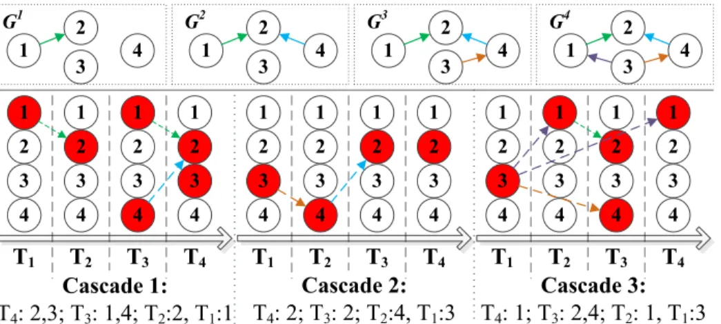
Overall, the basic idea of NETINF is that a pre-defined directed graph G supporting the underlying diffusion paths would lead to one or more consequent temporal sequences of activation between nodes, where in this work, "activation" of a node is equivalent to the emerging of a change point on it. The posterior probability of any single temporal sequence of the node activation (cascade) c is:

P c G ∝ _F∈F_d_(ƒ) _(j,k)‚l_Jβ∗ P_a(u, v), P_a u, v ∝ e[

∆e,K α , ∆

j,k= tk− tj (9)

As we have the collection of the cascades C from change points defined on reference variables by DICCCOL system through the whole scan time from each individual, and aim to infer the underlying directed graph G (functional pathway), goal would be to find a G that maximizes the posterior probability P(C|G) according to Eq. (6). An example case of the inference process is given in Fig. 2.2. The algorithm has been shown to be able to decrease the run time by several orders of magnitude without much loss in the solution quality [3]. The result of the NETINF algorithm is the directed graph G which characterizes the optimal functional pathway between variables supporting our observation of the sequence of change point detection results.

1 T1 2 3 4 T2 1 2 3 4 T3 1 2 3 4 1 2 3 4 T4 1 T1 2 3 4 T2 1 2 3 4 T3 1 2 3 4 1 2 3 4 T4 Cascade 1: T4: 2,3; T3: 1,4; T2:2, T1:1 Cascade 2: T4: 2; T3: 2; T2:4, T1:3 1 2 4 3 G1 1 2 4 3 G2 1 T1 2 3 4 T2 1 2 3 4 T3 1 2 3 4 1 2 3 4 T4 Cascade 3: T4: 1; T3: 2,4; T2: 1, T1:3 1 2 4 3 G3 1 2 4 3 G4

(20)

sequence figures at the bottom of the figure are the observations e.g. emerging time of change point detection results on the 4 variables from 3 subjects, where red indicates the existence of a change point on that variable at the corresponding time (T1-T4). The strings at the bottom are time stamps representation of the figure above. Thus the observation of the change points in each subject is a single cascade storing the time stamps of the change points of all its variables. The graphs G1-G4 at the top of the figure are the underlying pathways inferred by the greedy algorithm used in NETINF at each step, as it would iteratively add the edge that maximizes the marginal gain of the given observation (in this case, three cascades). Thus in G1, the algorithm would add edge connecting variable#1 and #2 to the empty graph, while in G2 it would add edge connecting variable#4 and #2. Note that marginal gain by adding an edge connecting two nodes that are temporally distant apart is smaller, as defined in Eq. 4, thus only in the third step it would add the edge connecting variable#3 and #4.

(21)

Chapter 3 Experimental Result

In this work, we used the HCP tfMRI dataset scanned during emotion task as an experimental data to test the performance of the proposed framework.

3.1. Cascade of change points inference simulation

Fig.3.1 Cascade of change points inference simulation. The real network (a) is unknown to the NETINF algorithm. We are given the contagions propagation time series data on each variable node, and aim to recover the network in figure (a). By using change point detection data generated from contagious signals, the NETINF algorithm recovers network (b). Red lines denote the mistakes.

(22)

To evaluate the accuracy of NETINF algorithm with the cascade of change points as input data, we designed a simulation test with a manually designed real network shown in Fig.3.1 (a). The contagious signals propagate inside the network are the pulse signals convolved with Haemodynamic Response Function (HRF), also we introduced Gaussian noise into the signal to simulate the brain fMRI signal of a certain variable point shown in Fig.3.2.

Fig.3.2. fMRI simulation signals within variable node 1 and variable node 2. The x-axis and y-axis represents the signal strength and time. The red line shows the signal in node 1 and the blue line shows the signal in node 2. Based on the real network, signals transferred from node 1 to node 2, therefore signal 2 depends on signal 1.

Since the contagions that spread among the variable nodes are based on the topology showed in Fig.3.1, by applying threshold change point detection method, what we get from the simulation signals are the timestamp cascades, by using the cascades as the input of NETINF algorithm, we get the network showed in Fig.3.1 (b). By using the simulation data, the NETINF recovers the network with a really high accuracy.

(23)

3.2. Data acquisition and pre-‐‑processing

In this work, we have used the tfMRI dataset of the emotion task from Human Connectome Project Q1 release, which is 2×2×2 isotropic high spatial resolution with high temporal resolution of TR=0.72 second. The scan length of the emotion task is 2 min 16 seconds (176 volumes). The preprocessing of the data has been conducted within the Q1 release, including motion correction, spatial smoothing, temporal pre-whitening, slice time correction and global drift removal. The details of the task experiment design and behavior measurements are referred to [1], and the detailed analysis of the data can be found in [2].

3.3. DICCCOL System result

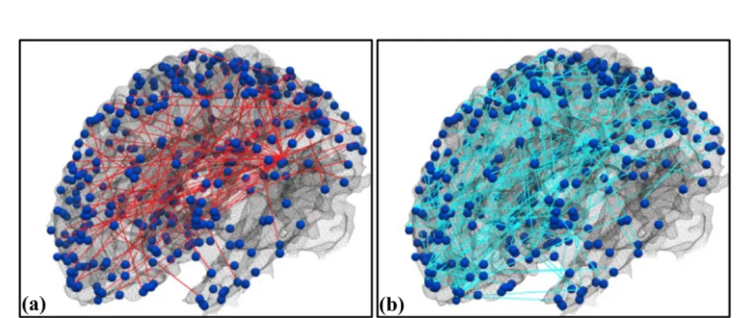
Fig. 3.3. Group-wise stable functional pathways inferred from emotion tfMRI data. The 358 DICCCOL ROIs are visualized on the cortical surface as dark blue spheres. (a) Positive functional pathways colored as red edges connecting DICCCOL ROIs. (b) Negative functional pathways colored as cyan edges.

The proposed method has been applied to infer the brain pathways of the brain regions defined by DICCCOL system in HCP Q1 release subjects. Based on the positive and negative sets of FCS and their corresponding change point detection results, the positive

(24)

negative brain pathways have been inferred respectively. Given the intrinsic correspondences of the DICCCOL system across different brains, as well as the fact that all the subjects were scanned during the same task, the change point detection results and the derived cascades on the DICCCOL-based connectomes can be readily pooled and integrated across all HCP subjects. By applying the NETINF algorithm on the collection of cascades from individuals, we have obtained the groupwise common pathway for both positive and negative functional connectivity propagations, as shown in Fig.3.3. It is evident that the positive (red) and negative (cyan) common pathways seldom overlap with each other, suggesting their distinct patterns over the cortex and the necessity to infer them separately.

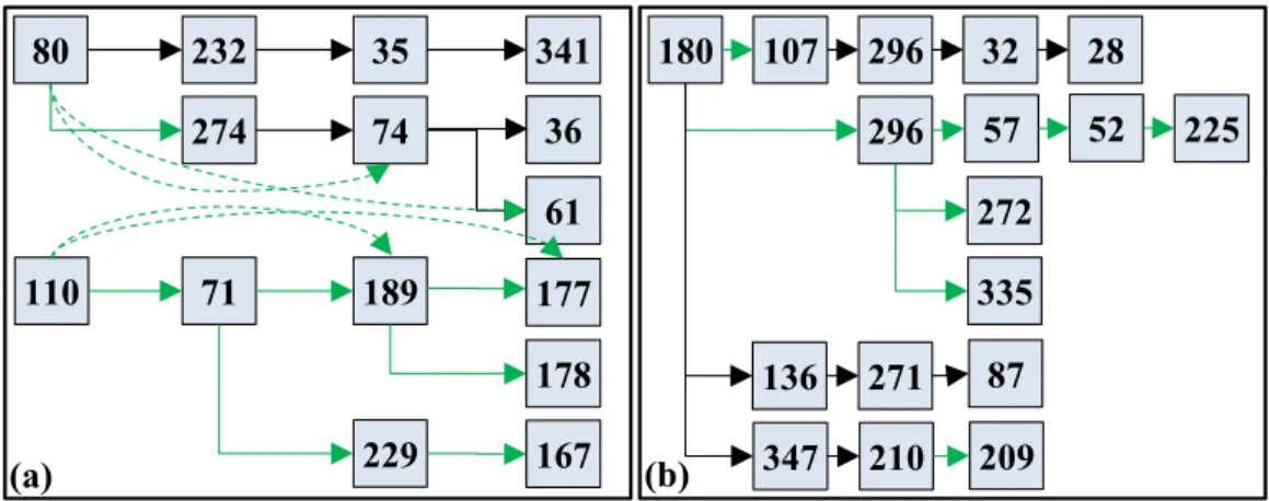
Fig. 3.4. (a) Illustration of the continuous positive functional pathways. The numbers of the hops in the figure are DICCCOL indices. Edges and dashed edges in green are pathways that are supported by strong structural connectivity measured by DTI data. (b) Similar illustration of the negative continuous functional pathways.

As the graph characterizing both the positive and negative common functional pathway contains more than one hundred edges, it is then important to identify the isolated continuous functional pathways. Major pathways from the positive connectivity dynamics and negative connectivity dynamics are illustrated in Fig. 3.4. It is interesting that DICCCOL #80 and #110 in positive networks and DICCCOL #180 in negative

180 107 296 32 28 296 57 52 225 272 335 136 271 87 347 210 209 80 232 35 341 74 36 61 178 229 167 274 110 71 189 177 (b) (a)

(25)

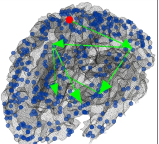
networks are serving as the connectivity propagation sources. A literature survey and meta-analysis shows that DICCCOL #110 is part of the emotion network identified by task-based activation detection. Given that the DICCCOL ROI#110 was inferred from the emotion task fMRI data, this result partly demonstrated that our framework is neuroscientifically meaningful. In addition, the DICCCOL ROI#80 has been shown to be part of the default mode network (DMN) based on concurrent resting state fMRI dataset, which is in agreement with literature report [10] that DMN nodes tend to play key roles in functional brain dynamics including serving as the originators of functional dynamics. We have also examined the structural connectivities between DICCCOL nodes based on the Diffusion Tensor Imaging (DTI) data, and found that there exist strong and consistent function pathways going from DICCCOL ROI#80 and 110, as illustrated by the green lines in Fig. 3.4. As shown in part of Fig. 3.5, the first continuous functional pathway starts from DICCCOL ROI#80, then goes through #232 (Frontal Lobe-Precentral Gyrus), #35 (Occipital Lobe-Lingual Gyrus) then ends at #341 (Frontal Lobe-Medial Frontal Gyrus). Considering the strong association of DICCCOL ROI#232, #35 and #341 with the working memory, visual memory encoding and social cognition respectively, this pathway could be the major consequence of transferring the visual input into short-term memory, then into higher-order social cognitive funcitons in the brain. Another major pathway starts from DICCCOL ROI#80 goes through #274 (Frontal Lobe-Superior Frontal Gyrus), #74 (Parietal Lobe-Angular Gyrus) then ends at either #36 (Occipital Lobe-Superior Occipital Gyrus) or #61 (Parietal Lobe-Precuneus). DICCCOL ROI #274 and #74 are mostly related to visual perception and its processing, while #61 is specifically associated with shape cognition. As the Emotion task design is consist of alternatively-presented emotion face blocks and shape blocks, it is interesting to find the two pathways originated from DICCCOL ROI#80 cover the major cognitive process during the Emotion task, while following two totally different route.

(26)

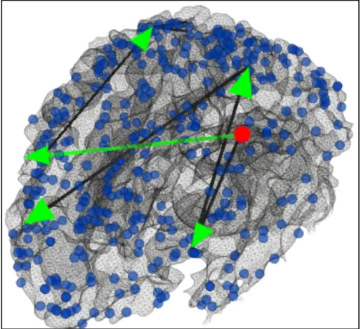
Fig. 3.5 Visualization of the continuous positive functional pathways starting from ROI#80 (red dot). Edges colored in green are also supported by strong DTI-derived structural connectivity.

On the other hand, postivie continuous functional pathway originated from DICCCOL ROI #110 would cover brain areas including #71 (Parietal Lobe-Inferior Parietal Lobule, main function is attention), #189 (Frontal Lobe-Precentral Gyrus, main function is also attention), #229 (Frontal Lobe-Precentral Gyrus, main function is emotional cognition) then end at #177 (Claustrum, main function is also emotional cognition), #178 (Limbic Lobe-Uncus, main function is long-term memory) or #167 (Limbic Lobe-Parahippocampal Gyrus, main function is also long-term memory), as shown in Fig. 3.6. This group of pathways are responsible for a different direction of brain fucntions comparing to the previous group: rather than decoding the visual input and processing it

(27)

at the corresponding site (emotion/shape cognition), this pathway starts from the emotion cognition center to the long-term memory encoding site.

Fig. 3.6 Visualization of the continuous positive functional pathways starting from ROI#110 (red dot).

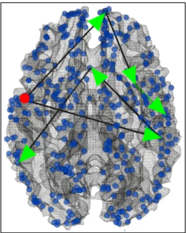
Similarly, we have analyzed the negative continuous functional pathways, which are unanimously originated from DICCCOL ROI #180. This ROI is located at Frontal Lobe-Precentral Gyrus, with main function is working memory, especially those related with emotion. The first group of functional pathways, as visualized in Fig. 3.7, goes through DICCCOL ROI #107 (Parietal Lobe-Inferior Parietal Lobule, main function is attention and cognition), #296 (Frontal Lobe-Middle Frontal Gyrus, main function is emotion sadness), #32 (Occipital Lobe-Lingual Gyrus, main function is emotion) then #28 (OccipitalLobe-Precuneus, main function is emotion disgusting). Considering the

(28)

vast majority of the regions involved are related with emotion processing, this pathway could be indicated as the transition between different emotion states induced by the task stimulus.

Fig. 3.7 Visualization of the first group of continuous negative functional pathways starting from ROI#180 (red dot). Edges colored in green are also supported by strong DTI-derived structural connectivity.

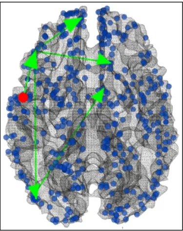
The second group of negative functional pathway goes through #296, #57, #52, then ends at #225, as shown in Fig. 3.8. DICCCOL ROI #296 has been discussed above which is related to sadness emotion, while the rest of regions are responsible for emotion fear (#57), action execution (#52), then incentive-elicited emotion cognition (#225). Similar

(29)

to the first group, this pathway could also indicate the transition between emotion states because of the many emotion-related regions invovled.

Fig. 3.8 Visualization of the second group of continuous negative functional pathways starting from ROI#180 (red dot). Edges colored in green are also supported by strong DTI-derived structural connectivity.

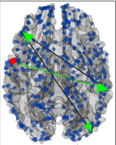
The third group of negative functional pathway goes through #347 (Frontal Lobe-Medial Frontal Gyrus, main function is vision perception and cognition), #210 (Temporal Lobe-Superior Temporal Gyrus, main function is emotoinal cognition), then ends at #209 (Temporal Lobe-Sub Gyral, main function is social cognition). As most of the regions involved are linked to cognition, this pathway could be interpreted as the information flow among cognitive regions as a response of emotion memory encoding/decoding.

(30)

Fig. 3.9 Visualization of the third group of continuous positive functional pathways starting from ROI#180 (red dot). Edges colored in green are also supported by strong DTI-derived structural connectivity.

(31)

Chapter 4 Conclusion

In this thesis, we have researched into the brain functional connectivity pathway inference problem. We developed a novel functional brain pathway inference framework for modeling functional brain dynamics. First, we defined the reference variables based on the DICCCOL system landmarks, then we modeled the dynamics of functional connectivity through sliding time window approach, By performing change point detection algorithm on the obtained connectivity strength and summarizing change point resutl data, we constructed the timestamp cascade that represents the brain functional activity. Finally, the dynamic connectivity propagation patterns between DICCCOLs were inferred by using a diffusion network inferring method (NETINF).

To evaluate our framework on time-series strength data similar to brain fMRI dataset, we designed a simulation on a small test network dataset, and showed that our model is able to accuratedly reveal the original network. In our practical experiments, the framework has been applied on the emotion task fMRI dataset of the publically available HCP Q1 release, and a set of consistent and neuroscientifically meaningful pathways such as the emotion-related and DMN nodes have been achieved. In general, our work has revealed novel insights into the functional brain dynamics and their structural pathways in the brain. Despite the considerable variability of such dynamics patterns across individuals, we also observed quite consistent and common patterns across this HCP Q1 population. We believe the framework we proposed is a promising step toward understanding brain’s

(32)

(33)

Chapter 5 Future Study

5.1. Using HAFNI atlases as reference variables

An alternative system for the reference variable definition is based on the full brain sparse coding result, in which the big voxel-wise fMRI data matrix is factorized into the multiplication of a dictionary matrix and the corresponding sparse loading coefficient matrix. In previous works [13] it has been found that the decomposed reference weight matrix naturally reveals the intrinsic functional network organization patterns among reconstructed brain networks and is reproducible across different tasks and individual brains. Thus the learned dictionaries from each individual fMRI dataset could be served as the effective representation of the comprehensive functional networks in cortical activities both in task and resting-state. If following the framework in [13] we can obtain 400 number of time series defined on the reference variables for each subject by performing the dictionary learning algorithm on their fMRI dataset. Fig 5.1 shows an attemptation of functional network pathway inference based on HAFNI reference variables of object 1. The details of the HAFNI system and the atlases obtained could be found at http://hafni.cs.uga.edu/.

(34)

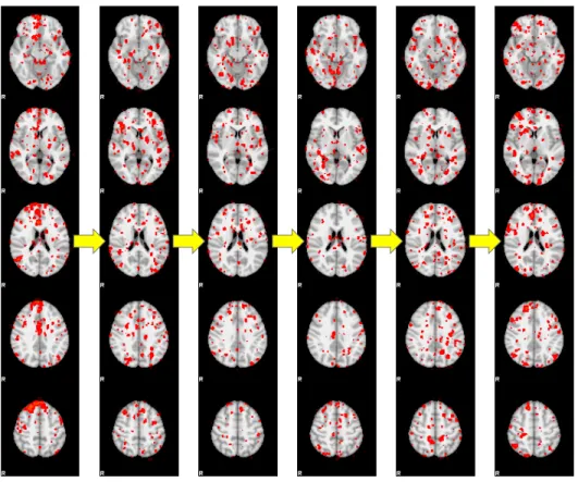
Fig. 5.1. One sample functional network pathway inferred from the positive functional connectivity strength dynamics of a randomly-selected subject. Each column in the figure is the spatial map of one network (out of the totally 400). The yellow arrow indicates the transition between networks in the pathway.

5.2. Other future work directions

We have several possible interesting directions for future work. In our current framework, we are only using the change point information of different DICCCOL ROIs on the inference, using fMRI signal curve pattern to do the inference can give us more accurate estimation.

(35)

Bibliography

[1] Barch, D.M., et al., Function in the human connectome: Task-‐fMRI and individual differences in behavior. NeuroImage, 2013. 80(0): p. 169-‐189.

[2] Van Essen, D.C., et al., The WU-‐Minn Human Connectome Project: An overview. NeuroImage, 2013. 80(0): p. 62-‐79.

[3] Rodriguez, M.G., J. Leskovec, and A. Krause, Inferring networks of diffusion and

influence, in Proceedings of the 16th ACM SIGKDD international conference on Knowledge discovery and data mining2010, ACM: Washington, DC, USA. p. 1019-‐1028.

[4] Gilbert, C.D., Sigman, M.: Brain States, Top-‐Down Influences in Sensory Processing, Neuron, 54:677-‐696 (2007)

[5] Mumford, D.: On the computational architecture of the neocortex. I. The role of the thalamo-‐cortical loop, Biol. Cybern, 65:135-‐145 (1991)

[6] Mumford, D.: On the computational architecture of the neocortex.II. The role of corticocortical loops, Biol. Cybern, 66:241-‐251(1992)

[7] Chang, C., Glover, G.H.: Time-‐frequency dynamics of resting-‐state brain connectivity measured with fMRI, NeuroImage, 50(1):81-‐98, 2010.

[8] Smith, S.M., Miller,K.L., Moeller,S., et al.: Temporally-‐independent functional modes of spontaneous brain activity, PNAS, Feb. 7, 2012.

[9] Zhu, D., et al.: DICCCOL: Dense Individualized and Common Connectivity-‐Based Cortical Landmarks, Cerebral Cortex, Apr. 5 (2012)

[10] Peili Lv, Lei Guo, Xintao Hu, Xiang Li, Changfeng Jin, Junwei Han, Lingjiang Li,Tianming Liu, Modeling Dynamic Functional Information Flows on Large-‐scale Brain Networks, MICCAI 2013. [11] Jinglei Lv, Zhichao Lian, Xiang Li, Dajiang Zhu, Tianming Liu, Jing Zhang, Group-‐wize change point

(36)

detection in task FMRI data by Bayesian methods

[12] Li X, Lim C, Li K, Guo L, Liu T: Detecting brain state changes via fiber-‐centered functional connectivity analysis. Neuroinformatics, pp. 1–18.

[13] Jinglei Lv, Xi Jiang, Xiang Li, Dajiang Zhu, Shu Zhang, Shijie Zhao, Hanbo Chen, Tuo Zhang, Xintao Hu, Junwei Han, Jieping Ye, Lei Guo, Tianming Liu Holistic Atlases of Functional Networks and Interactions Reveal Reciprocal Organizational Architecture of Cortical Function IEEE Transactions on Biomedical Engineering, 2015. vol. 62(4), pp. 1120-‐1131.

[14] Mason M, Fan G, Plath K, Zhou Q, Horvath S (2009) Signed weighted gene coexpression network analysis of transcriptional regulation in murine embryonic stem cells. BMC Genomics 10: 327+ [15] Tu Z, Wang L, Arbeitman MN, Chen T, Sun F (2006) An integrative approach for causal gene identification and gene regulatory pathway inference. Bioinformatics 22: e489–e496.

[16] Neal, 1993. R. M. Neal, Probabilistic Inference Using Markov Chain Monte Carlo methods, Tech. Rep. CRG-‐TR93-‐1, University of Toronto, Department of Computer Science, 1993

[17] http://gerardkeegan.com/glossary/cerebral-‐cortex

[18] http://www.inside-‐r.org/packages/cran/minet/docs/mrnet

[19] Andrew R, Nitesh C, Scott E (2013) A Survey of Current Integrative Network Algorithms for System Biology. Systems Biology: Integrative Biology and Simulation Tools: pp 479-‐495

[20] Yixuan Yuan, Xi Jiang, Dajiang Zhu, Hanbo Chen, Kaiming Li, Peili Lv, Xiang Yu, Xiaojin Li, Shu Zhang, Tuo Zhang, Xintao Hu, Junwei Han, Lei Guo, Tianming Liu (2013) Meta-‐analysis of Functional Roles of DICCCOLs, Neuroinformatics, 2013. Vol. 11(1), pp. 47-‐63.

(37)

Appendix A

Function Source Code

A.1 NETINF_WindowCorr2D.m

% NETINF_WindowCorr2D.m

% Ruichen Dai % 10/10/2015

% Find the positive and negative correlation functional connectivity strength from the correlations obtained from each reference variable of the given subject.

function NETINF_WindowCorr2D(file_Input, length_Window, string_Task, string_Sbj)

mtx_Input = load(file_Input);

[count_ROI, count_Obv] = size(mtx_Input); if (count_Obv == 400)

mtx_Input = mtx_Input';

[count_ROI, count_Obv] = size(mtx_Input); end

(38)

mkdir(dir_Output);

count_TotalWindow = count_Obv -‐ length_Window + 1;

mtx_WindowCorr2DSummed_P = zeros(count_ROI, count_TotalWindow); mtx_WindowCorr2DSummed_N = zeros(count_ROI, count_TotalWindow); mtx_Diag = eye(count_ROI, count_ROI);

for i = 1 : count_TotalWindow

mtx_InputWindow = mtx_Input(:, i : i + length_Window -‐ 1); % The correlation significance is not currently considered; %[mtx_Corr, mtx_PVal] = corr(mtx_InputWindow');

[mtx_Corr, ~] = corr(mtx_InputWindow'); mtx_Corr(isnan(mtx_Corr)) = 0; mtx_Corr(mtx_Diag > 0) = 0; mtx_Corr_Positive = mtx_Corr; mtx_Corr_Positive(mtx_Corr < 0) = 0; mtx_Corr_Negative = mtx_Corr; mtx_Corr_Negative(mtx_Corr > 0) = 0; mtx_Corr_Negative = abs(mtx_Corr_Negative);

% The correlation significance is not currently considered; %mtx_PVal(isnan(mtx_PVal)) = 0; %mtx_Significant = mtx_PVal < 0.05; %mtx_Corr = mtx_Corr.*mtx_Significant; vct_CorrSigSum_P = sum(mtx_Corr_Positive); vct_CorrSigSum_N = sum(mtx_Corr_Negative);

(39)

mtx_WindowCorr2DSummed_N(:, i) = vct_CorrSigSum_N; end

file_Output_P = ['../EMOTION/', string_Sbj, '/', 'sbj_', string_Sbj, '_', string_Task, '_corrSumP_HAFNI_All.txt'];

DataIO_MTX2TXT(mtx_WindowCorr2DSummed_P, file_Output_P);

file_Output_N = ['../EMOTION/', string_Sbj, '/', 'sbj_', string_Sbj, '_', string_Task, '_corrSumN_HAFNI_All.txt'];

DataIO_MTX2TXT(mtx_WindowCorr2DSummed_N, file_Output_N);

for j = 1 : count_ROI

vct_Output_P = mtx_WindowCorr2DSummed_P(j, :)'; vct_Output_P = vct_Output_P -‐ mean(vct_Output_P);

file_Output_P = ['../EMOTION/', string_Sbj, '/', 'sbj_', string_Sbj, '_', string_Task, '_corrSumP_HAFNI_', Tool_Int2Index(j, 3), '.txt'];

DataIO_MTX2TXT(vct_Output_P, file_Output_P); vct_Output_N = mtx_WindowCorr2DSummed_N(j, :)'; vct_Output_N = vct_Output_N -‐ mean(vct_Output_N);

file_Output_N = ['../EMOTION/', string_Sbj, '/', 'sbj_', string_Sbj, '_', string_Task, '_corrSumN_HAFNI_', Tool_Int2Index(j, 3), '.txt'];

DataIO_MTX2TXT(vct_Output_N, file_Output_N); end

(40)

A.2 NETINF_generatescript.m

% NETINF_generatescript.m

% Ruichen Dai % 10/12/2015

% Generate shell scripts to prepare for the change point detection process

function NETINF_generateScript(string_Task, string_Sbj, count_Obs)

file_batchSH = ['/home/share/TmpData/xiang/netinf/EMOTION/CPdetection/', string_Sbj, '_', string_Task, '.sh']; fileID = fopen(file_batchSH, 'w'); for j=1:400 string_HAFNI = Tool_Int2Index(j, 3);

string_FileNameN = ['./EMOTION/', string_Sbj, '/sbj_', string_Sbj, '_', string_Task, '_corrSumN_HAFNI_', string_HAFNI, '.txt'];

file_blockLabelN = ['./EMOTION/', string_Sbj, '/block_label_sbj_', string_Sbj, '_', string_Task, '_corrSumN_HAFNI_', string_HAFNI, '.txt']; file_TraceN = ['./EMOTION/', string_Sbj, '/trace_sbj_', string_Sbj, '_', string_Task, '_corrSumN_HAFNI_', string_HAFNI, '.txt'];

string_Script = ['./MCMC_empty ', string_FileNameN, ' ', num2str(count_Obs), ' 1 100 hyper_par.txt ', file_blockLabelN, ' ', file_TraceN, ' 1 -‐1 init_', num2str(count_Obs), '.txt'];

fprintf(fileID, string_Script); fprintf(fileID, '\n');

string_FileNameP = ['./EMOTION/', string_Sbj, '/sbj_', string_Sbj, '_', string_Task, '_corrSumP_HAFNI_', string_HAFNI, '.txt'];

(41)

file_blockLabelP = ['./EMOTION/', string_Sbj, '/block_label_sbj_', string_Sbj, '_', string_Task, '_corrSumP_HAFNI_', string_HAFNI, '.txt']; file_TraceP = ['./EMOTION/', string_Sbj, '/trace_sbj_', string_Sbj, '_', string_Task, '_corrSumP_HAFNI_', string_HAFNI, '.txt'];

string_Script = ['./MCMC_empty ', string_FileNameP, ' ', num2str(count_Obs), ' 1 100 hyper_par.txt ', file_blockLabelP, ' ', file_TraceP, ' 1 -‐1 init_', num2str(count_Obs), '.txt'];

fprintf(fileID, string_Script); fprintf(fileID, '\n'); end fclose(fileID); fclose all; end

A.3 NETINF_calculatePost.m

% NETINF_calculatePost.m % Ruichen Dai % 11/05/2015

% Calculate the change point detection for each subject

function [mtx_PostP, mtx_PostN] = NETINF_batchPost2MTX(string_Task, string_Sbj)

mtx_Post = zeros(137, 400); for j=1:400

(42)

file_Temp = ['./post_block_label_sbj_', string_Sbj, '_', string_Task, '_corrSumP_HAFNI_', string_HAFNI, '.txt']

vct_Temp = importdata(file_Temp); mtx_PostP(:, j) = vct_Temp;

file_Temp = ['./post_block_label_sbj_', string_Sbj, '_', string_Task, '_corrSumN_HAFNI_', string_HAFNI, '.txt']

vct_Temp = importdata(file_Temp); mtx_PostN(:, j) = vct_Temp; end mtx_PostP(mtx_PostP<1) = 0; mtx_PostP= mtx_PostP'; mtx_PostP(:, 1) = 0; mtx_PostN(mtx_PostN<1) = 0; mtx_PostN = mtx_PostN'; mtx_PostN(:, 1) = 0; end

A.4 NETINF_batchPost2MTX.m

% NETINF_batchPost2MTX.m % Ruichen Dai % 10/12/2015

(43)

function [mtx_PostP, mtx_PostN] = NETINF_batchPost2MTX(string_Task, string_Sbj)

mtx_Post = zeros(137, 400); for j=1:400

string_HAFNI = Tool_Int2Index(j, 3);

file_Temp = ['./post_block_label_sbj_', string_Sbj, '_', string_Task, '_corrSumP_HAFNI_', string_HAFNI, '.txt']

vct_Temp = importdata(file_Temp); mtx_PostP(:, j) = vct_Temp;

file_Temp = ['./post_block_label_sbj_', string_Sbj, '_', string_Task, '_corrSumN_HAFNI_', string_HAFNI, '.txt']

vct_Temp = importdata(file_Temp); mtx_PostN(:, j) = vct_Temp; end mtx_PostP(mtx_PostP<1) = 0; mtx_PostP= mtx_PostP'; mtx_PostP(:, 1) = 0; mtx_PostN(mtx_PostN<1) = 0; mtx_PostN = mtx_PostN'; mtx_PostN(:, 1) = 0; end

(44)

A.5 NETINF_generatecascade.m

% NETINF_batchPost2MTX.m

% Ruichen Dai % 10/12/2015

% generate the cascade based on the change point matrix

function NETINF_generateCascade(mtx_PostP, mtx_PostN, string_Sbj, string_Task)

file_Cascade_P = ['./cascade_sbj_', string_Sbj, '_', string_Task, '_P.txt'];

fileID_P = fopen(file_Cascade_P, 'w'); for j=0:399

fprintf(fileID_P, [num2str(j), ',', num2str(j)]); fprintf(fileID_P, '\n');

end

fprintf(fileID_P, '\n'); string_timeStamp = ''; for i=137:-‐1:1

idx_HAFNI = find(mtx_PostP(:, i) == 1); idx_HAFNI = idx_HAFNI-‐1;

count_HAFNI= length(idx_HAFNI); string_Time = num2str(i);

for j=1:count_HAFNI

string_timeStamp = [string_timeStamp, num2str(idx_HAFNI(j)), ',', string_Time, ';']; %#ok<AGROW>

end end

(45)

string_timeStamp(end) = []; fprintf(fileID_P, string_timeStamp); fprintf(fileID_P, '\n'); fclose(fileID_P);

file_Cascade_N = ['./cascade_sbj_', string_Sbj, '_', string_Task, '_N.txt'];

fileID_N = fopen(file_Cascade_N, 'w'); for j=0:399

fprintf(fileID_N, [num2str(j), ',', num2str(j)]); fprintf(fileID_N, '\n');

end

fprintf(fileID_N, '\n'); string_timeStamp = ''; for i=137:-‐1:1

idx_HAFNI = find(mtx_PostN(:, i) == 1); idx_HAFNI = idx_HAFNI-‐1;

count_HAFNI= length(idx_HAFNI); string_Time = num2str(i);

for j=1:count_HAFNI

string_timeStamp = [string_timeStamp, num2str(idx_HAFNI(j)), ',', string_Time, ';']; %#ok<AGROW>

end end

string_timeStamp(end) = [];

(46)

fprintf(fileID_N, '\n'); fclose(fileID_N); fclose all; end

A.6 simu_main.m

% simu_main.m % Ruichen Dai % 08/20/2015

% the main function used to simulate the change point detection data used in netinf algorithm global table table = zeros(11,1); initPulse1 = zeros(1,20); initPulse2 = zeros(1,20); initPulse3 = zeros(1,20); initPulse4 = zeros(1,20); initPulse5 = zeros(1,20); initPulse6 = zeros(1,20); initPulse7 = zeros(1,20); initPulse8 = zeros(1,20); initPulse9 = zeros(1,20);

(47)

initPulse10 = zeros(1,20); initPulse11 = zeros(1,20); for t = 2 :20 initPulse7(t) = simulation(7,3); initPulse6(t) = simulation(6,2); initPulse5(t) = simulation(5,2); initPulse4(t) = simulation(4,2); initPulse3(t) = simulation(3,1); initPulse2(t) = simulation(2,1); initPulse1(t) = simulation(1,1); initPulse7(t) = simulation(7,8); initPulse9(t) = simulation(9,11); initPulse11(t) = simulation(11,10); initPulse10(t) = simulation(10,8); initPulse9(t) = simulation(9,8); initPulse8(t) = simulation(8,8); end addpath C:\Users\eruidai\Documents\MATLAB\spm\spm12 pulse1 = fMRI_HRF(initPulse1, 12, 8, 16); NOISE1=randn(size(pulse1)); NOISE1=NOISE1-‐mean(NOISE1); signal_power = 1/length(pulse1)*sum(pulse1.*pulse1);

(48)

noise_variance = 4 * signal_power / ( 13^(10/10) ); NOISE1=sqrt(noise_variance)/std(NOISE1)*NOISE1; pulse1 = pulse1 + NOISE1;

pulse1 = pulse1'; pulse2 = fMRI_HRF(initPulse2, 12, 8, 16); NOISE1=randn(size(pulse2)); NOISE1=NOISE1-‐mean(NOISE1); signal_power = 1/length(pulse2)*sum(pulse2.*pulse2); noise_variance = 4 * signal_power / ( 13^(10/10) ); NOISE1=sqrt(noise_variance)/std(NOISE1)*NOISE1; pulse2 = pulse2 + NOISE1;

pulse3 = pulse3';

pulse4 = fMRI_HRF(initPulse4, 12, 8, 16); NOISE1=randn(size(pulse4));

NOISE1=NOISE1-‐mean(NOISE1);

(49)

pulse6 = pulse6'; pulse7 = fMRI_HRF(initPulse7, 12, 8, 16); NOISE1=randn(size(pulse7)); NOISE1=NOISE1-‐mean(NOISE1); signal_power = 1/length(pulse7)*sum(pulse7.*pulse7);

(50)

pulse9 = pulse9'; pulse10 = fMRI_HRF(initPulse10, 12, 8, 16); NOISE1=randn(size(pulse10)); NOISE1=NOISE1-‐mean(NOISE1); signal_power = 1/length(pulse10)*sum(pulse10.*pulse10);

(51)

pulse11 = pulse11'; plot(pulse1,'b'); hold on;

plot(pulse2, 'r');

save C:\Users\eruidai\Documents\MATLAB\short5_pulse1 pulse1 save C:\Users\eruidai\Documents\MATLAB\short5_pulse2 pulse2 save C:\Users\eruidai\Documents\MATLAB\short5_pulse3 pulse3 save C:\Users\eruidai\Documents\MATLAB\short5_pulse4 pulse4 save C:\Users\eruidai\Documents\MATLAB\short5_pulse5 pulse5 save C:\Users\eruidai\Documents\MATLAB\short5_pulse6 pulse6 save C:\Users\eruidai\Documents\MATLAB\short5_pulse7 pulse7 save C:\Users\eruidai\Documents\MATLAB\short5_pulse8 pulse8 save C:\Users\eruidai\Documents\MATLAB\short5_pulse9 pulse9 save C:\Users\eruidai\Documents\MATLAB\short5_pulse10 pulse10

(52)

save C:\Users\eruidai\Documents\MATLAB\short5_pulse11 pulse11 postshort5 = [pulse1,pulse2,pulse3,pulse4,pulse5,pulse6,pulse7,pulse8,pulse9,pulse10 ,pulse11] changeP(postshort5) load result.mat

A.7 simu_dependency.m

% simu_dependency.m % Ruichen Dai % 08/20/2015

% the function that define the dependency of the simulation network function value = simulation(x,y)

global table table(x) = 0; value = 0; if ((x == 1 && y == 1) || (x == 8 && y == 8)) value = generator(0.25); table(x) = value; elseif (table(y) == 1) value = generator(0.6); table(x) = value; end end

(53)

function value = generator(possibility) x = rand(1,1); if x < possibility value = 1; else value = 0; end end

A.8 simu_changepointdetection.m

% simu_changepointdetection.m % Ruichen Dai % 08/20/2015

% the preliminary version of change point detection method used in simulation function changepointdetection(matrix) String = '' for j = 2 : length(matrix) for i = 1 : 11 if (matrix(j,i) - matrix(j-1,i) > 0.7) String = strcat(String,int2str(i),',',int2str(j),'; '); end end end

(54)

save path end

INFERRING BRAIN PATHWAYS OF DYNAMIC FUNCTIONAL CONNECTIVITY BY DIFFUSION AND INFLUENCE MODELING RUICHEN DAI. (Under the Direction of Tianming Liu)

Inferring brain pathways of dynamic functional

Connectivity by diffusion and influence modeling

Contents

List of Figures

Chapter 1

Introduction

1.1.

Brain function research

1.2.

Brain’s functional pathway inference: motivation

and design

Chapter 2

Material and Methods

2.1.

Method overview

2.2.

Reference variable definition by DICCCOL system

2.3.

Functional brain connectome and its dynamics

2.4.

Change points detection based on FCS dynamics

2.5.

Pathway inference from change point cascades

Chapter 3

Experimental Result

3.1.

Cascade of change points inference simulation

3.2.

Data acquisition and pre-­‐‑processing

3.3.

DICCCOL System result

Chapter 4

Conclusion

Chapter 5

Future Study

5.1.

Using HAFNI atlases as reference variables

5.2.

Other future work directions

Bibliography

Appendix A

Function Source Code

A.1 NETINF_WindowCorr2D.m

A.2 NETINF_generatescript.m

A.3 NETINF_calculatePost.m

A.4 NETINF_batchPost2MTX.m

A.5 NETINF_generatecascade.m

A.6 simu_main.m

A.7 simu_dependency.m

A.8 simu_changepointdetection.m

Data acquisition and pre-‐‑processing