Crystallographic texture approximation by quadratic programming

(1)

Crystallographic texture approximation by quadratic programming

Thomas Bo¨hlke

a,*

, Utz-Uwe Haus

b

, Volker Schulze

c

a

Otto-von-Guericke-Universita¨t Magdeburg, Institut fu¨r Mechanik, PSF 4120, 39016 Magdeburg, Germany

b

Otto-von-Guericke-Universita¨t Magdeburg, Institut fu¨r Mathematische Optimierung, PSF 4120, 39016 Magdeburg, Germany

c_{Volkswagen AG, EZVT Methodenplanung/Umformsimulation, Brieﬀach 1796/2, Germany}

Received 12 August 2005; received in revised form 24 October 2005; accepted 9 November 2005 Available online 19 January 2006

Abstract

This paper considers the problem of approximating a given crystallite orientation distribution function (codf) by a set of texture com-ponents. Problems of this type arise for example if the codf has to be reconstructed from discrete orientations or if one looks for a phys-ical interpretation of the codf. The same problem is encountered if crystallographic texture based constitutive models have to be speciﬁed. The equivalence of these tasks to a mixed integer quadratic programming problem (MIQP) – a standard but challenging problem in opti-mization theory – is shown. Special emphasis is given to the generation of a class of approximations with an increasing number of texture components. Furthermore, the constraints resulting from the non-negativity, the normalization, and the symmetry of the codf are ana-lyzed. Finally, a set of approximations of three diﬀerent experimental textures determined with this solution scheme is presented and discussed. Based on these hierarchical solutions, the engineer can decide in what detail the microstructure is considered.

Keywords: Crystallographic texture; One-point correlation function of crystal orientations; Orientation distribution function; Quadratic programming; Texture components

1. Introduction

Single phase polycrystals are composed of grains of the same material which differ with respect to their lattice orien-tations. The simplest statistical description of such micro-structures is based on the crystallite orientation distribution function (codf) which specifies the volume fraction of a mate-rial having a specific lattice orientation. The codf is the one-point correlation function of lattice orientation and describes the crystallographic texture in the material. Higher-order correlation functions allow for a description of the morpho-logical texture. The correlation functions can be estimated based on orientation data determined experimentally for example by X-ray diffraction or by automated electron back-scatter diffraction orientation measurements. For a review concerning the representation of microstructures of

polycrys-tals and the experimental determination of their mesoscale

microstructure see Adams and Olson[1].

Due to the general complexity of a codf it is often nec-essary to look for simpliﬁed, but physical, descriptions which are essentially low dimensional. In the context of crystallographic textures this was ﬁrst done by Wasserman

and Grewen[38], who introduced so called texture

compo-nents to describe textures peculiar to speciﬁc processing histories. A large amount of work has been done to formu-late isotropic and anisotropic model functions and to iden-tify the dominant components in experimental textures [22,17,16]. Texture components are used on the one hand to obtain a physical interpretation of experimental codfs and on the other hand to homogenize the mechanical behavior with an acceptable numerical eﬀort. Taylor type

material models [35,37,25,6,28] allow for a description of

the macroscopic mechanical behavior due to a speciﬁc slip system geometry and orientation distribution. From the numerical point of view, large scale ﬁnite element simula-tions of metal forming operasimula-tions based on the Taylor

* _{Corresponding author.}

E-mail addresses:[email protected](T. Bo¨hlke),haus@ mail.math.uni-magdeburg.de(U.-U. Haus),volker.schulze@volkswagen. de(V. Schulze).

www.actamat-journals.com Acta Materialia 54 (2006) 1359–1368

First published in:

EVA-STAR (Elektronisches Volltextarchiv – Scientific Articles Repository) http://digbib.ubka.uni-karlsruhe.de/volltexte/1000013737

(2)

model are very time-intensive and storage-consuming if the crystallographic texture is approximated by several

hun-dred discrete crystals. Therefore, Raabe and Roters [30]

introduced the so called texture component crystal plastic-ity method which describes crystallographic textures by small sets of discrete orientations. Due to the discontinuous approximation of the codf the approach by Raabe and

Roters[30]requires a random variation of the discrete

crys-tal orientation through the sample. In the approach by

Bo¨hlke et al.[4]texture components are described by

con-tinuous model functions. The eﬀective stress is obtained by integrating the crystal stress – weighted by the codf – over the orientation space. The two material models mentioned before require an approximation of the codf by discrete or continuous texture components. The method suggested in this paper yields both a discrete (taking only the main ori-entations into account) and a continuous approximation, in the last case also giving a rigorous error bound.

In some applications, the codf is already discretized into a ﬁnite set of weighted orientations. If the number of orien-tations needs to be reduced, the proposed method can be used to ﬁnd an optimal set of components to approximate the initial distribution.

In this paper we restrict our attention to the formulation as a mixed integer quadratic programming problem (MIQP) problem and its approximate solution without considering mechanical properties. These could only be predicted based on several simpliﬁcations and assumptions which themselves are still a subject under discussion. For the case of a continuous approximation of the codf a dis-cussion of eﬀective mechanical properties can be found

for example in Refs.[4,5].

The outline of the paper is as follows. After a short

review of existing approximation techniques in Section 2,

the basic features of the codf and its properties implied by crystal and sample symmetries are discussed in Sections 3 and 4. The concept of texture components is introduced

in Section 5 and speciﬁed for the case of the von Mises–

Fisher–Matthies distribution function, widely used in

texture analysis. Section 6 deals with the problem of

approximating a codf by a set of model functions. Special emphasis is given to constraints resulting from the require-ment of an approximation with a small number of texture components. It is shown that such a problem is equivalent to a deﬁnite mixed integer quadratic programming problem (MIQP). Optimization problems of such a type arise in rather diﬀerent contexts such as chemical process

optimiza-tion and portfolio optimizaoptimiza-tion. Finally, in Secoptimiza-tion 7 the

approximation of three diﬀerent experimental textures based on this solution scheme is considered. It is shown that the applied solution procedure yields good approxima-tions in terms of quality and quantity.

2. Previous approaches

The problem of ﬁnding approximations for a given

tex-ture has been considered in detail by Kocks et al.[20], Toth

and Van Houtte[36], and Helming et al.[18]. The earliest

approach for discretizing a given codf was to put a nearly

equidistant grid on the Euler space in a 90 ·90 ·90

region. For each of the so deﬁned boxes the codf is integrated and the respective volume fraction is determined. Since the resulting number of boxes is usually too high for a subse-quent simulation, boxes with a volume fraction above a speciﬁed limit are selected and renormalized as the approximation of the codf. This cutting technique (CUT) has been analyzed and criticized by Toth and Van Houtte

[36]. The same authors suggest two new discretization

schemes in order to improve the CUT method. The first (sta-tistical) method (STAT) is based on a cumulative orientation distribution function which is used to map random numbers onto the orientation space such that for a large set of these numbers the texture is reproduced. The cumulative function is generated again based on a grid with a characteristic reso-lution. The only parameter of the algorithm (beside the aforementioned resolution) is the number of random orien-tations used for the approximation. The second technique – called the limited orientation distance (LOD) method – is also based on a grid on the orientation space. Intensities on grid points are transferred to points with higher intensi-ties if the distance between the points is smaller than a spe-cific value. The two parameters of this algorithm are the mesh size and the distance which governs the transfer. The authors analyze and compare both methods with respect to the (i) reproducibility of the codf, (ii) the prediction of effective mechanical properties, (iii) the prediction of defor-mation textures based on these discretization, and (iv) the effect of rediscretizations during deformation texture model-ing. It is shown that both methods are superior to the CUT method and that the LOD technique works better for the high intensity regions whereas the STAT method is better in regions where the intensity is low. The earlier approach

by Kocks et al.[20]used a random grid on the orientations

space and assigns suitable weights in an iterative procedure. A special approach for the approximation of steel

tex-tures was developed by Delannay et al. [11]. In this

approach the texture is characterized by a set of parame-ters, describing typical features of industrial steel sheets by prescribed fibers. The parameters vary the intensities, the fiber thickness and the position of the knots controlling the fibers. Another approach with standardized positions

and components is given by Cho et al.[9]. In this paper

the approximation is performed on a set of typical compo-nents for cubic metals. The compocompo-nents are located at ﬁxed points and described by von Mises–Fisher distributions with ﬁxed half-widths. The weight of the component is cal-culated similar to the LOD technique: the volume fraction of a component is equal to the sum of all intensities within a certain acceptance angle. These special approximation techniques depend strongly on the expertise of the user and are only suited to a special class of textures.

As an alternative a genetic approach by Tarasiuk et al.

[34] for identifying the texture components may also be

(3)

guarantee global optimality of their solution, and do not provide an error bound which would be of help in evaluat-ing their quality.

3. The crystallite orientation distribution function

A crystal orientation is described by a proper

orthogo-nal tensorQ=giei2SO(3) which is introduced in such a

way that it maps the ﬁxed reference basiseionto the lattice

vectorsgi.Qcan be parameterized by Euler angles/1=u1,

/2=U,/3=u2[8] ðQTÞ_ij ¼ C1C3S1C2S3 S1C3þC1C2S3 S2S3 C1S3S1C2C3 S1S3þC1C2C3 S2C3 S1S2 C1S2 C2 2 6 4 3 7 5; ð1Þ

where Ci and Si denote the values cosð/iÞ and sinð/iÞ,

respectively. The matrix components refer to the base

vec-torsei. The transposition is introduced in order to make the

description of crystal orientations byQ=gieicompatible

to the one introduced by Bunge[8].

The codff(Q) speciﬁes the volume fraction dv/vof

crys-tals having the orientationQ[7,31], i.e.

dv

v ðQÞ ¼fðQÞdQ; ð2Þ

dQis the volume element inSO(3) which ensures an

invari-ant integration overSO(3) [14], i.e.

Z SOð3Þ fðQÞdQ¼ Z SOð3Þ fðQQ₀ÞdQ 8Q₀2SOð3Þ. ð3Þ

IfSO(3) is parameterized by Euler angles, the volume

ele-ment dQis given by

dQ¼sinðUÞ

8p2 du1dUdu2. ð4Þ

The functionf(Q) is non-negative and normalized such that

fðQÞP0 8Q2SOð3Þ;

Z

SOð3Þ

fðQÞdQ¼1. ð5Þ

The orientation distribution functionf(Q) reﬂects both the

symmetry of the crystallites forming the aggregate and the sample symmetry, which results from the processing his-tory. The crystal symmetry implies the following symmetry

relation forf(Q)

fðQÞ ¼fðQHCÞ 8HC2SCSOð3Þ; ð6Þ

where SC denotes the symmetry group of the crystallite.

Similarly, the sample symmetry implies

fðQÞ ¼fðHSQÞ 8HS2SS SOð3Þ. ð7Þ

HereSSdenotes the symmetry group of the sample.

4. Elementary regions due to crystal and sample symmetries

The parameterization of the SO(3) with Euler angles

results in a periodic space with a natural period of 2p in

all parameters. This periodic cell consists of two equivalent asymmetric units, since a glide plane perpendicular to

U=pwith glide increments ofpinu1andu2exists

inher-ently in this parameterization[8]. Therefore a complete

pre-sentation of the Euler space is given by either one of the asymmetric units, for example

06_u

1<2p; 06U<p; 06u2<2p. ð8Þ

The application of the crystal and sample symmetry oper-ations results in a further reduction of the independent re-gion. The cubic group consists of 24 proper orthogonal transformations resulting in 24 equivalent units within

the range given by Eq.(8). InFig. 1a typical representation

of three anisotropic regions in au1-cut for cubic crystals is

shown [15].

These three prismatic regions are the result of the

three-fold symmetry axis atu2=p/4;U¼arccosð

ffiffiffi 3

p

=3Þof cubic

crystals, which results in a non-linear transformation within the Euler space. For the evaluation of the codf, the region 3 can be problematic since the singular plane

withU= 0 is included. Region 2 consists of two prismatic

parts connected only at the location of the threefold

sym-metry axis. Therefore the region 1 of Fig. 1 is favorable

for an identiﬁcation procedure. This region is given by

06_u 1<2p; Ul6U< p 2; 06u2< p 2; ð9Þ where Ul¼arccos min cosðu2Þ ffiffiffiffiffiffiffiffiffiffiffiffiffiffiffiffiffiffiffiffiffiffiffiffiffiffi 1þcos2_ð_u 2Þ p ; _{ffiffiffiffiffiffiffiffiffiffiffiffiffiffiffiffiffiffiffiffiffiffiffiffiffi}sinðu2Þ 1þsin2ðu₂Þ q 0 B @ 1 C A. ð10Þ

In the case of orthorhombic sample symmetry, which con-sists of a symmetry group of four elements, a reduction in

the u1-range to one quarter of the cubic case is possible.

Considering the same arguments as before, one elementary region is given by

Fig. 1. Elementary regions in au1-cut for cubic crystals (U,u22[0,p/2]) [15].

(4)

06_u 1< p 2; Ul6U< p 2; 06u2< p 2. ð11Þ 5. Texture components

Crystallographic textures can often be described by a small number of texture components or texture ﬁbers [38,8,21]. A texture component is a crystal orientation for which the codf shows a (local) maximum in the elemen-tary region. In the neighborhood, the codf is decreasing in an isotropic or anisotropic way. A commonly used model function, which describes a central distribution, is the von Mises–Fisher distribution. The von Mises–Fisher tribution has the maximum entropy of all orientation

dis-tributions onSO(3) with the expectation value ofQequal

to Qa. This distribution function was introduced by von

Mises in a two-dimensional case and by Fisher in a

three-dimensional case [23]. Matthies[26] was the ﬁrst to

apply the von Mises–Fisher distribution in texture analy-sis. He called it a normal distribution in the orientation

space see also [27], but this interpretation was criticized

by Schaeben [32,33]. Eschner [12] and Eschner and

Fun-denberger [13] used non-central distribution functions for

the description of experimental crystallographic textures. An overview of central and non-central distribution

func-tions onSO(3) can be found in the monograph by Mardia

and Jupp[23].

In the following the codff(Q) is approximated by a set

ofMmodel functionsga(Q) (a2{1,. . .,M}) and an isotropic

backgroundg0(Q) = 1"Q2SO(3). The model functions are

taken to be central distributionsga(Q) =g(Q,Qa,ba) atQa

with half-widths ba and with weights ma. We can hence

approximate f(Q) by a convex combination of the model

functionsga(Q): fðQÞ fðQÞ ¼X M a¼0 magðQ;Qa;baÞ ð12Þ with XM a¼0 ma¼1; maP0 8a20;. . .;M. ð13Þ

The value of a central distribution g(Q, Qa, ba) at Q

de-pends only on the distance x between Q and Qa, which

is generally given by xðQ;QaÞ ¼arccos 12ðtrðQQ 1 a Þ 1Þ ð14Þ

[8]. The von Mises–Fisher distribution is given by

gðQ;Qa;baÞ ¼NðSaÞexpðSacosðxðQ;QaÞÞÞ; ð15Þ where Na¼ 1 I0ðSaÞ I1ðSaÞ ð16Þ and Sa¼SðbaÞ ¼ lnð2Þ 2 sin2ðba=4Þ . ð17Þ

The modiﬁed Bessel functionsInare deﬁned by

InðSÞ ¼ 1

p

Z p 0

expðScosðtÞÞcosðntÞdt. ð18Þ

As mentioned before, the distribution functionf(Q) reﬂects

both the symmetry of the crystallites forming the aggregate and the sample symmetry. The following modiﬁed von Mises–Fisher distribution implies the fulﬁllment of the con-straint due to the crystal symmetry

gðQ;Qa;baÞ ¼ 1 24 X24 b¼1 NaexpðSacosðxðQHCbQ 1 a ÞÞÞ; ð19Þ

where theHC_b 2SOð3Þare the 24 elements of the symmetry

group of cubic crystals. Considering the sample symmetry for the orthorhombic case, the model function can be rewritten as gðQ;Q_a;baÞ ¼ 1 96 X24 b¼1 X4 c¼1 NaexpðSacosðxðHScQH C bQ 1 a ÞÞÞ ð20Þ

with the four elements of the orthorhombic group

HS_c 2SOð3Þ.

6. Identiﬁcation of the model functions

In the following an approximationfðQÞ(see Eq.(12)) of

f(Q) is deﬁned based on a set ofMgrid points on the

ele-mentary region. Each grid point represents the center of a von Mises–Fisher distribution. To each component a

half-width ba and a volume fraction ma is assigned. The

half-widths ba of the components are assumed to be identical

for all components. The aim is to identify fðQÞin terms

of the volume fractions ma such that fðQÞ approximates

the original codff(Q) with a small numberM06M. This

numberM06Mis limited by the computational eﬀort of

the application in which the approximation is used. For example in the case of ﬁnite element simulation of deep drawing processes the current computational power of the computers limits the total number of components to about 100 in the orientation space.

As a deﬁnition of the distance between the two functions

f(Q) andfðQÞwe deﬁne

D¼

Z

SOð3Þ

ðfðQÞ fðQÞÞ2dQ. ð21Þ

The distanceDcan be reformulated in the following setting

D¼I2X M a¼1 mahaþ XM a;b¼1 mambGab; ð22Þ

whereIdenotes the texture index

I¼

Z

SOð3Þ

(5)

The vectorhaand the matrixGabare given by ha¼ Z SOð3Þ fðQÞgaðQÞdQ; ð24Þ Gab¼ Z SOð3Þ g_aðQÞgbðQÞdQ. ð25Þ

In order to perform the integration over SO(3) (see Eqs.

(24) and (25)) the parameterization ofSO(3) is changed.

In-stead of using {u1,U,u2} the new variablefis introduced

byU= arccos(f). Then the metric becomes homogeneous

and an integral overSO(3) is given by

Z SOð3Þ fðQÞwðQÞdQ¼ 1 8p2 Z uu 2 0 Z uu 1 0 Z fu fl fðu1;UðfÞ;u2Þ wðu1;UðfÞ;u2Þdu1dfdu2 ð26Þ with uu 1¼2p f l_¼₁ _fu_{¼ þ}₁ _ð₂₇_Þ and uu₂¼2p UðfÞ ¼arccosðfÞ. ð28Þ

Due to the cubic crystal symmetry and the orthorhombic sample symmetry the range of integration can be reduced

to [0,p/2]3. In that range a Gaussian quadrature scheme

is applied with 36 Gauss points in each direction.

Using these deﬁnitions it is apparent that we have to solve a quadratic programming problem (QP), namely

min 2X M a¼1 mahaþ XM a;b¼1 mambGab subject to X M a¼1 ma¼1 maP0 8a2M ð29Þ

withM¼ f1;. . .;Mgand the additional restriction that at

mostM0of the variablesmamay be positive in the solution.

We can model this requirement by introducingM binary

variablessawhich are to be 1 ifma> 0. This can be

accom-plished by the constraintssaPma. Adding the set packing

constraintPM_a_¼₁sa6M0now guarantees that at mostM

vol-ume fractions are positive, i.e. non-zero, in a solution. The

problem of identifyingfðQÞis thus solved by the MIQP:

min 2X M a¼1 mahaþ XM a;b¼1 mambGab subject to saPma XM a¼1 ma¼1 XM a¼1 sa6M0 maP0 8a2M sa2 f0;1g 8a2M ð30Þ

Note that the matrix Gab is by its deﬁnition positive

deﬁ-nite. The problem(29)as well as its variant with an upper

bound on the number of positive variables (30) is of a

similar structure to the well-known question of evaluating risk versus reward in the context of a portfolio of ﬁnancial

assets ﬁrst described by Markowitz [24]. A successful

computational study of the latter has been performed by

Bienstock[3]. The signiﬁcant diﬀerence of Eq.(30)in

com-parison to the instances arising in portfolio optimization is

that the matrix Ghas full rank. Therefore the solution of

the problem turns out to be much more diﬃcult than the typical ﬁnancial problems: the individual QP problems are solved slower, and the number of nodes that must be visited in the branch-and-bound tree is high.

Various reliable methods are available for solving the

quadratic programming problem(29), namely Newton-type

feasible descent methods, Lagrange-multiplier methods, logarithmic barrier methods, and primal-dual interior point

methods. For an overview see Bertsekas[2]. The latter two

classes are particularly suited to the deﬁnite quadratic pro-gramming problems we are dealing with. The mixed-integer

quadratic programming problems like (30) are in general

much harder to solve than their continuous counterparts, and one can often only resort to branch-and-bound methods.

7. Numerical examples

As an illustration of the outlined procedure, a fit of three typical automotive deep drawing steel grades is performed. Due to the final steps of the manufacturing process of steel sheets, which consist of cold rolling and subsequent anneal-ing, the materials have practically orthorhombic sample symmetry. The measurement of the codf was performed by means of a pole figure measurement with X-ray diffrac-tion on three lattice planes and a subsequent recalculadiffrac-tion

of the codf using the series expansion method [8] up to

L= 22.

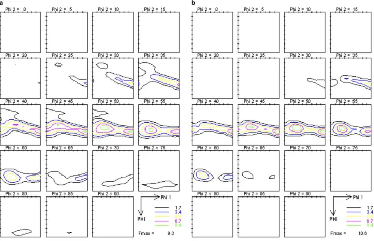
The ﬁrst example is DX53, a mild deep drawing steel grade. This material is dominated by a ﬁber texture close

to the c-ﬁber, which is given in Euler angles by

(06_u₁_{< 90}_;_U_{= 54.7}_,_u₂_{= 45}_{). In}_{Fig. 2}_{(a) the}

mea-sured codf of the material is shown. The other material is a high-strength micro-alloyed steel grade, H340LAD. In this

case, the dominant structure is thea-ﬁber, which is located

at (u1= 0; 06U< 90,u2= 45), whereas the c-ﬁber is

less pronounced. The measured codf is given in Fig. 3(a).

Beside the differences in the dominant fiber directions, the materials have significantly different peak values.

Both textures were ﬁtted with a grid of 5within the

ele-mentary region by components with a half-width of

ba= 6. For a reduction of the processed data, a

prelimin-ary selection of the ansatz functions is performed. For the optimization procedure, only grid points are considered, which have an intensity that is higher than a certain limit value, similar to the CUT method. This preliminary data reduction is performed only to reduce the subsequent pro-cessing time, it is not a mandatory part of the approxima-tion process. For this example, the limit was set to 50% of the maximum value of the measured codf. This limits the

(6)

Fig. 2. Texture measurement and approximation with 24 components of DX53. (a) Measurement and (b) approximation.

(7)

number of ansatz functions toM= 95 in case of DX53 and

M= 92 in case of H340LAD. Within this set of ansatz

functions, the optimization with respect to an optimum

weight for a given numberM0of functions is performed.

We used the commercial solver software CPLEX [19]

which employs a logarithmic barrier algorithm to solve the initial quadratic optimization problems within less than 6 s on a 1.2 GHz Ultrasparc-IV processor. In addition, for

each material a sequence of instances of type(30)was

gen-erated, the limit M0 on the number of positive variables

varying between 1 and 24. Solving these instances to opti-mality using CPLEX within reasonable computation time was impossible except for the smallest instances. However, using solver settings that employ heuristics to ﬁnd good

solutions early in the solution process (mip emphasis 3

andmip strategy variableselect 3), we were able to identify a series of good solutions together with proven bounds on their maximum optimality gap. We also tested

the Xpress[10]solver, but found it to be inferior, especially

in application to the MIQP problems.

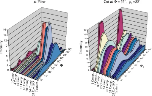
The result of the optimization process is a number of components and their respective weights that approximate the given texture. For these examples, a number of such representations was selected starting with one component up to 24 components, given by the model function of Eq.

(20). For a better comparison, cuts along two important

directions, the a-ﬁber and a cut at (06_u₁_{< 90}_,

u1= 55; U= 55, u2= 55) were chosen for the

evalua-tion of the approximated codf. In these cuts, the

domi-nant components of both textures are located or

intersecting. The results are presented in Fig. 4 for the

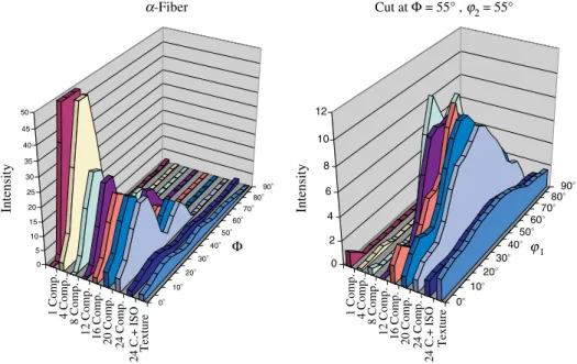
DX53 and in Fig. 5 for the H340LAD. In both cases

the ﬁrst component ﬁts the maximum peak of the mea-sured codf. With every additional component, the

approx-imation of the measured distribution improves with an increasing number of ansatz functions. The intensity of the major components is reduced and secondary features start to develop, which can be observed especially in the case of H340LAD.

Using only the identiﬁed major components, the result-ing texture is too anisotropic, therefore the values of the codf are overestimated in the peak regions. The approxi-mation improves if the inforapproxi-mation about the remaining isotropic part is also used in the ﬁt. The introduction of this

additional component is seamless both in Eqs. (29) and

(30), where no decision variable needs to be introduced

for it. With this ‘‘isotropic’’ component added to the tex-ture approximation, the dominant values are in the range

of the measured texture. In the Figs. 4 and 5this result is

plotted for the case of 24 components next to the measured texture.

In Figs. 2(b) and 3(b) the codf plots for the ﬁtted tex-tures with 24 components and the isotropic part are pre-sented. The comparison with the measured codf shows that not only the dominant components are reproduced but also that the structure of the secondary regions is approximated suﬃciently, when the isotropic part is included in the approximation result.

One of the advantages of using MIQP techniques to solve these problems is that an error bound is available at any time: during the course of the branch-and-bound algorithm QP relaxations for the remaining subproblems are solved. The worst objective value among them is then

a safe lower bound for the original problem. Fig. 6

illus-trates the development of the gap between the objective function value for the best known solution (after 100,000 nodes of branch-and-bound) and the lower bound at that time, for both DX53 and H340. The absolute value of

0° 10° 20° 30° 40° 50° 60° 7080° ° 90° 0 2 4 6 8 10 12 14 16 Intensity Φ

1 Comp. 4 Comp. _{8 Comp.}

12 Comp.

24 C.+ ISO Texture a-Fiber 0° 10° 20° 30° 40° 50° 60° 70° 80° 90° 0 5 10 15 20 25 30 35 40 45 50 Intensity

12 Comp.

16 Comp. 20 Comp. _{24 Comp.} 24 C.+ ISO Texture

Cut at Φ= 55°,j₂=55°

j₁

(8)

the slope for the graph of the solutions is smaller for H340, indicating that the weaker texture is harder to approximate with few components.

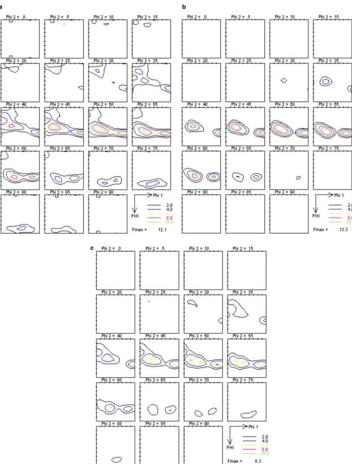
As a last example, the case of H220PD is considered. This material is a phosphorus-alloyed steel with a good formability and an intermediate strength. The texture

mea-surement (Fig. 7(a)) shows a dominant ﬁber structure close

to thec-ﬁber. A secondary feature is the branching of this

ﬁber in the vicinity of thea-ﬁber. For the approximation, a

limit was set to 20% of the maximum intensity, resulting in

M= 250 ansatz functions. The QP problem (Eq. 29) for

this material can be solved within 0.5 s. With varying

com-ponent limit M02{1,. . .,24}, and limited to 100,000 nodes

of branch-and-bound, the MIQP problems took on aver-age 4500 s. The approximation with 24 components is

given inFig. 7(b).

The main components of the ﬁber structure are repro-duced well, but the branching is not reprorepro-duced. This

eﬀect is caused by the limitation of the number M0 of

ansatz functions. The procedure described above ﬁts the ansatz functions to the main components of the texture. The examples above showed that this approximation improved with an increasing number of components, also reproducing secondary texture features. To approximate more complex textures with a small set of functions, one can introduce an additional requirement: volume

fractions selected in a solution of Eq. (30) should not

be clustered too closely. The criterion selected was that

the spherical angle, given by Eq. (14) between any two

volume fractions present in a solution of Eq.(30) should

be at least 7.5. Note that this imposes a stable set or

node packing condition on the volume fractions: Deﬁne a graph containing all volume fractions as nodes, with

two nodes a and b connected by an edge if

°ðQa;QbÞ67:5. Then we can model the additional

con-straints using the edge-node formulation of the stable set

polytope [29]:

saþsb61 for each pair ða;bÞwith°ðQa;QbÞ67:5.

ð31Þ

Introducing this distance criterion, the selected compo-nents are forced to a wider distribution, resulting in a better

approximation of the secondary features (Fig. 7(c)). The

spread in the weightsmaincreases to a factor of three

be-tween the smallest and the largest weight in the set. Since

the volume fraction of the isotropic componentm0is

dom-inated by the regions of low intensities, the peak values are underestimated. The addition of the stable set conditions increases computation time signiﬁcantly, to an average 6830 s over the 24 instances considered.

-2.5 -2 -1.5 -1 -0.5 0 5 10 15 20 25 -1.3 -1.2 -1.1 -1 -0.9 -0.8 -0.7 -0.6 -0.5 objective DX53 objective H340 component limit Mo Bound for DX53 Solution for DX53 Bound for H340 Solution for H340 QP Bound for DX53 and H340

Fig. 6. Error estimation for DX53 and H340LAD.

0° 10° 20° 30° 40° 50° 60° 70° 80° 90° 0 5 10 15 20 25 30 35 40 45 50 Φ

12 Comp.

16 Comp. 20 Comp. _{24 Comp.} 24 C.+ ISO Texture a-Fiber 0° 10° 20° 30° 40° 50°60 ° 7080° ° 90° 0 2 4 6 8 10 12 Intensity Intensity

12 Comp.

24 C.+ ISO

Texture

Cut at Φ= 55°,j₂_{= 55}°

j1

(9)

Fig. 7. Texture measurement and approximation of H220PD. (a) Measurement; (b) approximation without distance criterion; (c) approximation with distance criterion.

(10)

8. Summary

We have presented a method to approximate a texture with a hierarchical set of texture components using a solu-tion scheme based on the (semidefinite) mixed integer qua-dratic programming method. This approach is not limited to a special texture class nor to a specific sample or crystal symmetry configuration. The procedure enables the identi-fication of an optimum combination of ansatz functions for

a prescribed numberM0of components in a set. If the

com-putation is stopped prematurely, an error bound for the current state of the approximation is given.

A ﬁtting of typical steel textures with a small number of components was performed. The approximation repro-duces the measured textures with a tendency to cluster in regions of high intensities. If a wider distribution of the ansatz functions is needed, a distance based discrimination procedure can be added, which improves the approxima-tion of secondary texture features.

Acknowledgments

T. Bo¨hlke acknowledges the partial support rendered by the Deutsche Forschungsgemeinschaft (DFG) under grant GK 828. U.-U. Haus was supported by grant FOR-468 of the Deutsche Forschungsgemeinschaft. V. Schulze acknowledges the support by the Volkswagen PhD-program.

References

[1] Adams B, Olson T. The mesostructure-properties linkage in poly-crystals. Progr Mater Sci 1998;43:1–88.

[2] Bertsekas DP. Non-linear programming. Belmont, MA: Athena Scientiﬁc; 1995.

[3] Bienstock D. Computational study of a family of mixed-integer quadratic programming problems. Math Program 1996;74(2):121–40. [4] Bo¨hlke T, Risy G, Bertram A. A texture component model for anisotropic polycrystal plasticity. Computat Mater Sci 2005;32:284–93.

[5] Bo¨hlke T, Risy T, Bertram A. A texture based model for polycrystal plasticity. In: Proceedings of the 14th international conference on textures of materials (ICOTOM-14); 2005.

[6] Bronkhorst C, Kalidindi S, Anand L. Polycrystalline plasticity and the evolution of crystallographic texture in fcc metals. Roy Soc Lond A 1992;341:443–77.

[7] Bunge H-J. Zur Darstellung allgemeiner Texturen. Z Metallkd 1965;56:872–4.

[8] Bunge H-J. Texture analysis in material science. Go¨ttingen: Cuviller Verlag; 1993.

[9] Cho J-H, Rollett AD, Oh KH. Determination of volume fractions of texture components with standard distributions in euler space. Metall Mater Trans A 2004;35A:1075–86.

[10] Dash Optimization, 1999–2004. Dash optimization. Available from:

http://www.dashoptimization.cm/.

[11] Delannay R, Van Houtte P, Van Bael A, Vanderschueren D. Application of a texture parameter model to study planar anisotropy of rolled steel sheets. Model Simul Mater Sci Eng 2000;8:413–22.

[12] Eschner T. Texture analysis by means of model functions. Text Microstruct 1993;21:139–46.

[13] Eschner T, Fundenberger J. Application of anisotropic texture components. Text Microstruct 1997;28:181–95.

[14] GelÕfand I, Minlos R, Shapiro Z. Representations of the rotation and Lorentz groups and their applications. Oxford: Pergamon Press; 1963.

[15] Hansen J, Pospiech J, Lu¨cke K. Tables for texture analysis of cubic crystals. Berlin: Springer; 1978.

[16] Helming K. Texturapproximation durch Modellkomponenten. Go¨t-tingen: Cuvillier Verlag; 1996.

[17] Helming K, Eschner T. A new approach to texture analysis of multiphase materials using a texture component model. Cryst Res Technol 1990;25:K203–8.

[18] Helming K, Schwarzer R, Rauschenbach B, Geier S, Leiss LB, Wenk H-R, et al. Texture estimates by means of components. Z Metallkd 1994;85:545–53.

[19] ILOG, 1997–2004. Ilog, inc.,. CPLEX. Available from: http:// www.ilog.com/products/cplex/.

[20] Kocks U, Kallend J, Biondo A. Accurate representation of general textures by a set of weighted grains. Text Microstruct 1991;14– 18:199–204. iCOTOM 9, Special Issue.

[21] Kocks U, Tome C, Wenk H. Texture and anisotropy: preferred orientations in polycrystals and their eﬀect on materials proper-ties. Cambridge: Cambridge University Press; 1998.

[22] Lu¨cke K, Pospiech J, Jura J, Hirsch J. On the representation of orientations distribution functions (codfs) by model functions. Z Metallkd 1986;77:312–21.

[23] Mardia K, Jupp P. Directional statistics. New York, NY: John Wiley & Sons Ltd.; 2000.

[24] Markowitz H. Portfolio selection. J Finance 1952;7:77–91.

[25] Mathur K, Dawson P. On modeling the development of crystallo-graphic texture in bulk forming processes. Int J Plast 1989;5:67–94. [26] Matthies S. Standard functions in texture analysis. Phys Stat Sol B

1980;101:K111–5.

[27] Matthies S, Muller J, Vinel G. On the normal distribution in the orientation space. Text Microstruct 1988;10:77–96.

[28] Miehe C, Schro¨der J, Schotte J. Computational homogenization in ﬁnite plasticity. Simulation of texture development in polycrystalline materials. Comp Meth Appl Mech Eng 1999;171:387–418.

[29] Padberg M. On the facial structure of set packing polyhedra. Math Program 1973;5:199–215.

[30] Raabe D, Roters F. Using texture components in crystal plasticity ﬁnite element simulations. Int J Plast 2004;20:339–61.

[31] Roe R. Description of crystalline orientation of polycrystalline materials. III. General solution to pole ﬁgure inversion. J Appl Phys 1965;36:2024–31.

[32] Schaeben H. ‘‘Normal’’ orientation distribution. Text Microstruct 1992;19:197–202.

[33] Schaeben H. Diskrete mathematische Methoden zur Berechnung und Interpretation von kristallographischen Orientierungsdichten. Ober-ursel: DGM Informationsgesellschaft; 1994.

[34] Tarasiuk J, Wierzbanowski K, Bacroix B. Texture decomposition into gauss-shaped functions: classical and genetic algorithm methods. Computat Mater Sci 2004;29:179–86.

[35] Taylor G. Plastic strain in metals. J Inst Metals 1938;62:307–24. [36] Toth L, Van Houtte P. Discretization techniques for orientation

distribution functions. Text Microstruct 1992;19:229–44.

[37] Van Houtte P. A comprehensive mathematical formulation of an extended Taylor-Bishop-Hill model featuring relaxed constraints, the Renouard-Winterberger theory and a strain rate sensitive model. Text Microstruct 1988;8(9):313–50.

[38] Wasserman G, Grewen J. Texturen metallischer Werkstoﬀe. Berlin: Springer; 1962.