Prediction of expected performance for a genetic programming classifier

(1)

Prediction of expected performance for a genetic

programming classifier

Yuliana Martı´nez1•_{Leonardo Trujillo}1•

Pierrick Legrand2•_{Edgar Galva´n-Lo´pez}3

Received: 29 September 2015 / Revised: 7 February 2016 / Published online: 22 February 2016

ÓSpringer Science+Business Media New York 2016

Abstract The estimation of problem difficulty is an open issue in genetic pro-gramming (GP). The goal of this work is to generate models that predict the expected performance of a GP-based classifier when it is applied to an unseen task. Classification problems are described using domain-specific features, some of which are proposed in this work, and these features are given as input to the predictive models. These models are referred to as predictors of expected performance. We extend this approach by using an ensemble of specialized predictors (SPEP), dividing classification problems into groups and choosing the corresponding SPEP. The proposed predictors are trained using 2D synthetic classification problems with balanced datasets. The models are then used to predict the performance of the GP classifier on unseen real-world datasets that are multidimensional and imbalanced. This work is the first to provide a performance prediction of a GP system on test data, while previous works focused on predicting training performance. Accurate predictive models are generated by posing a symbolic regression task and solving it with GP. These results are achieved by using highly descriptive features and including a dimensionality reduction stage that simplifies the learning and testing

& Leonardo Trujillo

[email protected] Yuliana Martı´nez [email protected] Pierrick Legrand [email protected] Edgar Galva´n-Lo´pez [email protected] 1

Tree-Lab, Posgrado en Ciencias de la Ingenierıá, Departamento de Ingenierıá Elećtrica y Electrońica, Instituto Tecnolo´gico de Tijuana, Tijuana, BC, Mexico

2

CQFD Team, INRIA Bordeaux, IMB, Universite´ of Bordeaux, Talence, France

3

School of Computer Science and Statistics, Trinity College Dublin, Dublin, Ireland DOI 10.1007/s10710-016-9265-9

(2)

process. The proposed approach could be extended to other classification algorithms and used as the basis of an expert system for algorithm selection.

Keywords Problem difficultyPrediction of expected performance Genetic programmingSupervised learning

1 Introduction

Within the field of evolutionary computation (EC) [6] it is not yet clear if a particular algorithm will perform well on a specific problem instance. The ‘‘No Free Lunch’’ (NFL) theorem [70] has provided valuable theoretical and conceptual insights, broadly stating that all search algorithms on average are equivalent when they are evaluated over all possible problems. On the other hand, the NFL theorem does not apply to many common domains of genetic programming (GP) [43], a promising theoretical insight that drives research to develop the best possible GP-based search. Nevertheless, it is by now evident that most GP-based systems tend to perform well on some problem instances while failing on others, with little understanding as to why or when either of those two scenarios will arise [14,15,34,57,59].

The above issue can be described as the study of problem difficulty, which has been studied in different ways in EC and GP literature. Some methods focus on analyzing the properties of a problem’s fitness landscape [27]. This can be done, for instance, by defining specific classes of functions [20], or by extracting high-level features [14,15,34,57,59] or statistical properties [4,8,9,13,26,47,62,69] of the fitness landscape. In the case of standard tree-based GP, where search operators are applied in syntax space, the concept of a fitness landscape is difficult to define given that there is no clear way of determining a general concept of neighborhood for GP representations that are usually highly redundant, which limits the usefulness of such approaches. While some methods have been successfully applied to GP, these are mostly sampling-based techniques that attempt to infer specific types of structures within the underlying fitness landscape, such as: neutrality [8,11,12,42,

72], locality [9, 10], ruggedness [62], deception [56], fitness distance correlation (FDC) [4,56], fitness clouds [64] and negative slope coefficient (NSC) [66,67]. In this work, we refer to such methods as evolvability indicators (EIs), which are extensively reviewed in [33] and discussed in the following section.

One notable shortcoming of EIs is that they require an extensive sampling of the search space in order to compute them [2,46,65,68]. This is an important limitation: if we need to know when a particular problem is easy or difficult for an algorithm to solve it may just be easier to run the algorithm and observe its behavior and outcome. Therefore, some researchers have proposed predictive models that take the problem data (or a description of the data) as input, and produce as output a prediction of expected performance, we will refer to such methods as predictors of expected performance (PEPs). Currently, the development of PEPs represents the minority of research devoted to problem difficulty in GP, with only a few recent works. In particular, Graff and Poli [14–18] have studied the development of such predictive models, for symbolic regression, Boolean and time-series problems. While their

(3)

original work mostly focused on synthetic benchmarks [15], more recent contribu-tions extended their approach to performance prediction in real-world problems [14,

18]. However, in their approach it is necessary to have an extensive knowledge of the real-world problems in advance. Furthermore, their models are intended to predict the performance of the best solution found by GP on the training set of data, they did not address the prediction of performance on unseen test cases.

This paper is an extension of our previous work [57,59,60] where PEPs were first proposed for a GP classifier, making several methodological and experimental contributions. First, the PEP models are produced using only simple 2D synthetic datasets that are randomly generated. Second, the PEP models are used to predict the performance of the GP classifier on the test set of data, while previous works mostly focused on predicting performance on the training or learning set [14–18]. Third, accurate predictions are obtained on unseen real-world problems that are multidimensional and contain imbalanced data. On the other hand, previous works [14–18,57,59,60] used the same type of problems (either synthetic or real) for both training and testing. Fourth, to increase PEP accuracy this paper presents an ensemble approach using specialized PEP models called SPEPs. Each SPEP is trained to predict performance within a specific range of classification error. To do so, we use a two-tier approach, where each problem is first classified into a specific group, and then prediction is obtained from the corresponding SPEP which was trained for that group of problems. Finally, it is reasonable to state that the proposed approach could be applied to predict the performance of GP on other learning problems.

The remainder of this paper proceeds as follows. Section2reviews related work and Sect.3 provides a short survey of GP-based classification. The basic PEP strategy is outlined and evaluated in Sect. 4. Afterwards, Sect.5 introduces the proposed ensemble strategy based on SPEPs and provides experimental results. Finally, Sect.7 contains conclusions and future work.

2 Related work

Determining problem difficulty has been an important issue in EC for several years [35]. From an algorithmic perspective, problem difficulty can be related to the total runtime (or memory) required to find an optimal solution. Recently, He et al. [20] took this view one step further, to analytically define broad classes of fitness functions which allowed them to demonstrate that easy functions define unimodal fitness landscapes, while hard functions define deceptive landscapes for a (1?1) ES. However, it is important to remember that the difficulty of a particular problem depends upon the solution method. Therefore, in what follows we will try to limit our overview to GP-related research.

2.1 Evolvability indicators

The fitness landscape has dominated the way geneticists think about biological evolution and has been adopted by the EC community as a way to visualize

(4)

evolution dynamics [71]. Formally, a fitness landscape can be defined as a triplet (x;v;f), wherexis a set of configurations,vis a notion of neighborhood, distance or accessibility onx, andfis a fitness function [54]. The local and global structure of the fitness landscape describes the underlying difficulty of a search. However, in the case of standard GP [30] the concept of a fitness landscape is not clearly defined [27]. To overcome this, some works have constructed synthetic problems; such as the Royal Tree problem [44] or the K-landscapes model [62], where the goal of the search is defined as a particular tree structure with a specific syntax. Unfortunately, such models are not realistic since the space of possible programs is highly redundant [30] in most domains, and the goal is not a particular syntax but a particular expected output, also known as semantics [36, 63]. Therefore, some researchers have proposed variants of GP that explicitly account for program semantics. In semantic space the fitness landscape is clearly defined and unimodal. This has lead researchers to develop specialized search operators that modify program syntax while geometrically bounding the semantics of the generated offspring, this is known as geometric semantic GP (GSGP) [38]. Nevertheless, such approaches are still problematic since the size of the evolved programs grows exponentially with every generation, a limitation that is not easily solved [50]. This work will focus on measures of problem difficulty for standard GP systems [29], but could be applied to other supervised learning systems including GSGP.

In general, most meta-heuristics work under the assumption that the fitness of a candidate solution, a point on the fitness landscape, is positively correlated with the fitness of its (some) neighbors. Such a property can be defined as theevolvabilityof a landscape [1,41]. EIs extract a numerical indicator of a specific property of the fitness landscape to provide a measure of the evolvability within the landscape. Malan et al. [33] presents a comprehensive survey of EIs and other forms of fitness landscape analysis.

Those that have been studied in GP literature include neutrality [8,26], locality [9,

47], ruggedness [25, 62], fitness distance correlation (FDC) [4, 24, 56], fitness clouds [69] and the negative slope coefficient (NSC) [64]. While these approaches can sometimes provide good estimates of problem difficult for GP, they suffer from two practical limitations. First, for each new problem instance they require a large amount of data, by sampling the search space or performing several runs. Second, they cannot estimate the actual quality of the solution found, which can be important if we want to choose the best algorithm to use for a new problem, and if such a choice must be made in real-time. Indeed, Malan et al. [33] point out that a possible way forward is to build a mapping that can estimate algorithm performance based on a set of descriptive features of the problem, an approach that would provide a more practical measure of problem difficulty and allow us to choose the best algorithm for the specific task. Malan and Engelbrecht [32] attempted to find a link between EIs and algorithm performance for particle swarm optimization.

2.2 Performance prediction

PEPs predict the performance of a GP search on an unseen problem instance without performing the search or sampling the solution space. These models have been

(5)

derived using a machine learning approach [14,15,34,57,59]. The performance of GP on a set of problems and a description of those problems are used to pose a supervised learning task. A promising feature of PEPs is that they are not only useful for GP, they can also be used to predict the performance of other algorithms [16,59].

Graff and Poli [16] proposed linear predictive models based on a sampling of the fitness landscape, given by

PðtÞ a0þ

X

s2S

asdðs;tÞ; ð1Þ

wherePðtÞ is the predicted performance, t is the target functionality, dðs;tÞ is a distance measure,1 S is the set of all possible program outputs, also known as semantic space [38], and where each s represents the vector of program outputs obtained from the set of fitness cases used to define a particular problem, also known as the semantics of the program [36]. In other words, Graff and Poli [16] derive PEPs by sampling semantic spaceS. These models were tested on symbolic regression and 4-input Boolean problems with promising results.

The second and more recent approach towards building a PEP focuses on the problem data [14,17,18,34,57–60] and proceeds as follows. Assume we want to solve a supervised learning problempwith a GP search, where fitness is given by a cost function that must be minimized, such as an error measure. Let us define the performance of the GP algorithm as the associated error of the best solution found during training when it is evaluated on a particular set of fitness casesT, call this quantityFTðpÞ. The goal is to predict FTðpÞ, so first we construct a feature vector

b¼ ðb1;b2;. . .;bNÞ of N distinct features that describe the main properties of p.

Then, a PEP is functionKsuch that

FTðpÞ KðbÞ: ð2Þ

Notice that the form ofKis not a priori restricted in any way. Graff and Poli [17] use a linear function similar to the one used in their previous work [16]. Using this approach the feature vector b should be designed specifically for the domain of p. For example, features designed for symbolic regression and Boolean problems are proposed in [17], and the results show that the predictive accuracy surpasses that of the fitness-based models proposed in [16]. However, their work did not scale well to real-world cases. For instance, in [14, 18] the authors built PEPs to predict performance on real-world problems, but require information obtained from runs performed on similar problem instances, models built with simpler synthetic problems could not be used. It was not trivial to map multidimensional problems to the proposed feature space since the training problems were much simpler with a small number of dimensions. It would be impractical to consider all possible dimensionalities during training. This is an important limitation in building PEPs, since it is not trivial to have all the possible versions of the same problem. More-over, in the proposals made by Graff and Poli [14,17,18] the models predicted the

1 _{Such a distance measure is a common fitness function for many application domains of GP, particularly}

(6)

performance of the GP system on the training set of fitness cases; i.e., Twas the training set. While certainly of importance, performance on the training set may not be useful if the algorithm overfits the training examples, which happens often in real-world scenarios.

In previous work [57, 59, 60], we used a similar approach to predict the performance of a GP-classifier using descriptive features that characterize the geometry of the data distribution in feature space. The PEPs where built using quadratic linear models and non-linear GP models, the latter achieving the best performance on synthetic problems. However, it was not clear how well the PEPs generalized to unseen problem instances, particularly to real-world problems with imbalanced datasets and larger feature spaces than those used to train the models, a similar difficulty pointed out in [14, 18]. The current work extends our previous contributions by performing the learning process on 2D synthetic problems and testing on a wide variety of real-world datasets. Moreover, an important contribution of this work is that the PEP models are used to predict the performance of the best solution found by GP when it is evaluated on the test set of data. To achieve improved performance this work also proposes a two-tiered ensemble approach using specialized PEP models and a preprocessing stage for dimension-ality reduction.

3 Classification with GP

In machine learning one of the most common tasks is supervised classification [28]. The general task can be stated as follows. Given a patternx2RPassign the correct class label among C distinct classes x1;. . .;xC, using a training set T of

P-dimensional patterns with a known label. The idea is to build a mapping gðxÞ:RP_!_C_{, that assigns each pattern}_x _{to a corresponding class}_x

i, where g is

derived based on the evidence provided byT. GP has been widely used to address this problem [40, 53, 57, 73–75]. In general, GP can be applied to classification following three general approaches:

1. Feature selection and construction [39,40,48,57,75]. 2. Model extraction [3,55,61,73,74].

3. Learning ensemble classifiers [21,23,30].

Feature selection and construction is also known as preprocessing of the problem data. These approaches use GP to either select the most interesting problem features or to construct new features that simplify the classification problem. These techniques are often described as either filter [19, 39, 57, 75] or wrapper approaches [40,48,51]. In the former, feature construction is done independently of the model used to build the classifier, while in the latter fitness assignment is based on the performance of a classifier. On the other hand, model extraction with GP is used to build specific types of classifiers, such as decision trees [55, 61], classification rules [3, 45] and discriminant functions [74]. Finally, ensemble

(7)

classifiers are used to improve the quality of the classification task by using not only a single classifier, but a group of them, each one providing a different output [21,

23,30].

3.1 Probabilistic genetic programming classifier

In this work we derive PEPs for the probabilistic genetic programming classifier (PGPC) proposed in [75], a feature construction method. PGPC was chosen due to its simplicity and strong performance on real-world problems [53]; while other GP-based classifiers could have been used this is left as future work. In PGPC, GP is used to evolve a mappinggðxÞ:RP!Rthat transforms each input patternxinto a point on the real line. Furthermore, it is assumed that the behavior of g can be modeled using multiple Gaussian distributions, each corresponding to a single class [75]. The distribution of each class N ðl;rÞ is derived from the examples provided for it in setT , by computing the meanland standard deviationrof the outputs obtained fromg on these patterns. Then, from the distributionN of each class a fitness measure can be derived using Fisher’s linear discriminant; for a two class problem it proceeds as follows. After the Gaussian distributionN for each class are derived, a distance is required. In [75], Zhang and Smart propose a distance measure between both classes as

d¼2jl1l2j

r1þr2

; ð3Þ

wherel1andl2are the means of the Gaussian distribution of each class, andr1and

r2 their standard deviations. When this measure tends to 0, it is the worst case

scenario because the mappings of both classes overlap completely, and when it tends to1, it represents the optimal case with maximum separation. To normalize the above measure, the fitness for an individual mappingg is given by

fd ¼

1

1þd: ð4Þ

After executing PGPC, the best individual found determines the parameters for the Gaussian distributionNi associated to each class. Then, a new test pattern x is

assigned to classi whenNi gives the maximum probability; performance is

mea-sured by the total classification error (CE) on test data.

4 PEP: predictor of expected performance

The general goal of this work is to build models that can predict the performance of a GP-classifier (PGPC) without executing the search or sampling the problem’s search space. The general proposal is depicted in Fig.1, where for a given classification problem we do the following. First, apply a preprocessing step to simplify the feature extraction process and deal with multidimensional represen-tations. Second, perform feature extraction to obtain an abstraction of the problem.

(8)

Third, use a PEP model that takes as input the extracted features and produces as output the predicted classification error (PCE) on the testing set.

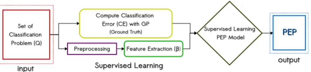
Moreover, to derive the PEP models we use a supervised learning methodology, depicted in Fig.2. This process takes as input a set of synthetic classification problemsQ and produces as output the PEP model as follows:

1. Compute the average classification error (CEl) on the test data by PGPC for eachp2 Q.

2. Apply a preprocessing for dimensionality reduction using principal component analysis (PCA), and take the first m principal components to represent the problem data.

3. Perform feature extraction on the transformed data using statistical and complexity measures to build a feature vectorbfor each p2 Q.

4. Finally, using the set of feature vector/performance pairs fðbi; CEliÞg

formulate a supervised symbolic regression problem and solve it using GP.

4.1 Synthetic classification problems

A set of synthetic classification problems was generated to learn our PEP models. Specifically, 500 binary classification problems were generated using Gaussian mixture models (GMMs) with either unimodal or multimodal classes, with different amounts of class overlap. All class samples lie within the closed 2-D interval x;y2 ½10;10, and 200 sample points were randomly generated for each class.

Fig. 1 Block diagram of the proposed PEP approach. Given a classification problem, the goal is to predict the performance of a GP classifier on the test data, in this case PGPC

Fig. 2 The methodology used to build the PEP model. Given a setQof synthetic classification problems:

(1) compute the CElof PGPC on all problems; (2) apply a preprocessing for dimensionality reduction;

(9)

The parameters for the GMM of each class were randomly chosen using a uniform distribution in the following ranges:

1. Number of Gaussian components:f1;2;3g.

2. Median of each Gaussian component for each dimension:½3;3.

3. Each element of the covariant matrix of each Gaussian component: (0, 2]. 4. The rotation angle of each covariance matrix: ½0;2p.

5. Proportion of samples generated with each Gaussian component: [0, 1].

4.2 PGPC classification error

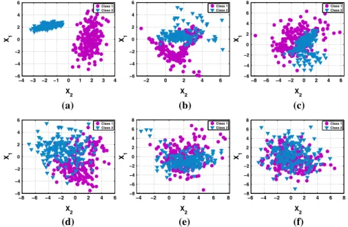
For each problem p2 Q we perform 30 runs of PGPC, randomly choosing the training and testing sets in each run. Then, the mean classification error CEl is computed by the average of the test performance achieved by the best solutions found in each run. The parameters of the PGPC system are given in Table1, a tree-based GP algorithm with dynamic depth bloat control [50], implemented using Matlab and the GPLAB toolbox [49]. Figure3 presents some examples, showing the problem data, the CElachieved by PGPC and the standard deviationrover all runs. The problems are ordered from the lowest CEl (easiest problem, depict in Fig.3a) to the highest, CEl(hardest problem, depict in Fig.3f).

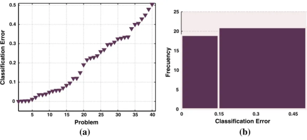
Figure4summarizes PGPC performance over all 500 synthetic problems in Q. Figure4a plots the CEl for each problem, ordered from the lowest to the highest error. On the other hand, Fig.4b shows an histogram of PGPC performance,

Table 1 Parameters for the PGPC algorithm

Parameter Description

Population size 200 Individuals

Generations 200 Generations

Initialization Ramped half-and-half, with six levels of maximum depth

Operator probabilities Crossoverpc¼0:8; mutationpl¼0:2

Function set n_þ;_;_{; =;}pﬃﬃ_;_sin_;_cos_;_log_;_xy_;_{j j;}_ifo

Terminal set fx1;. . .;xi;. . .;xPgwhere eachxiis a dimension of the data patternsx2RP

Bloat control Dynamic depth control

Initial dynamic depth 6 Levels

Hard maximum depth 20 Levels

Selection Tournament, size 3

Survival Keep best elitism

Training data 70 %

Testing data 30 %

(10)

quantifying how many problems are solved with a particular CEl. We arbitrarily set a threshold such that problems in the range 0 CEl0:15 are considered ‘‘easy’’ and the rest are considered to be ‘‘hard’’. From this perspective the plot reveals that randomly generated problems produce a biased distribution, where most problems are easy to solve. Since we intend to use this set to pose a supervised learning task, this would induce an unwanted bias. Therefore, we subsample Q to get a more

−4 −3 −2 −1 0 1 2 3 4 −6 −4 −2 0 2 4 6 X 2 X1 Class 1 Class 2 (a) (b) (c) (d) (e) (f) −2 0 2 4 6 −6 −4 −2 0 2 4 6 X 2 X1 Class 1 Class 2 −8 −6 −4 −2 0 2 4 6 −6 −4 −2 0 2 4 6 8 X 2 X1 Class 1 Class 2 −8 −6 −4 −2 0 2 4 6 −6 −4 −2 0 2 4 6 X₂ X1 Class 1 Class 2 −4 −2 0 2 4 6 8 −8 −6 −4 −2 0 2 4 6 8 X₂ X1 Class 1 Class 2 −6 −4 −2 0 2 4 6 8 −8 −6 −4 −2 0 2 4 6 8 X₂ X1 Class 1 Class 2

Fig. 3 The scatter plots show examples of synthetic classification problems, specifying the CEland

standard deviationrachieved by PGPC. These ordered from the lowest CEl(easiest depict in Fig.3a) to

the highest CEl (hardest depict in Fig. 3f). a CEl¼0r¼0. b CEl¼0:14r¼0:03. c

CEl¼0:17r¼0:03.dCEl¼0:21r¼0:03.eCEl¼0:36r¼0:04.fCEl¼0:46r¼0:04 50 100 150 200 250 300 350 400 450 500 0 0.1 0.2 0.3 0.4 0.5 Classification Error Problem (a) 0 0.15 0.3 0.45 0 50 100 150 200 250 300 Classification Error Frecuency (b)

Fig. 4 Performance of PGPC over all 500 synthetic problems inQ; whereashows the CElfor each

(11)

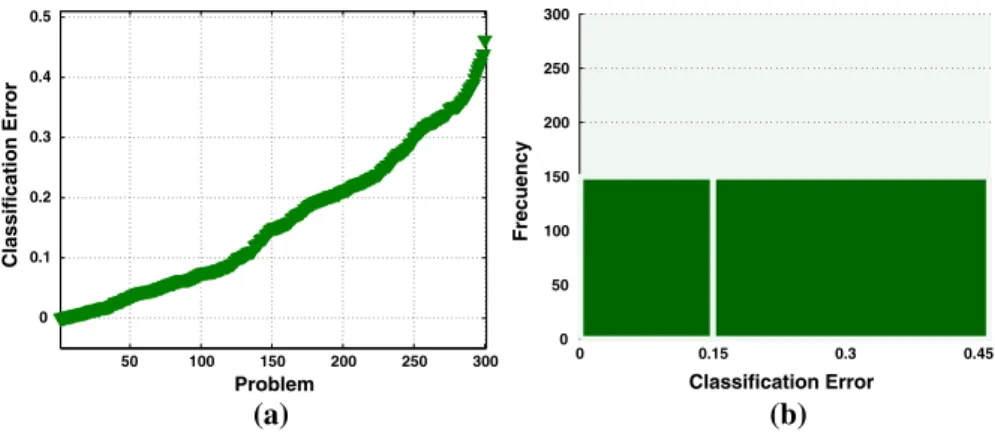
balanced distribution over CEl. The new set consists of 300 problems, and Fig.5

summarizes PGPC performance over this new setQ0. Notice that the performance plot for Q0 Q is similar to the one obtained for Q (see Fig.5a), but now the distribution over CElis flat (Fig.5b), providing a more balanced learning set. 4.3 Preprocessing

Previous work has found that PEP models can predict GP performance accurately for small scale synthetic problems [15–17,34,57–60], but accuracy degrades for real-world problems with high dimensional data [14,18]. This is due to the fact that feature extraction (the next step in the PEP approach) fails at extracting meaningful information in high dimensional spaces [14,18]. To deal with this issue, we apply a dimensionality reduction preprocessing of the problem data using PCA [5]. We propose to take the first m principal components to represent the data of each problem. In particular, we setm¼2 in all experiments reported here. In this way, all problems are reduced to the same number of dimensions used in the synthetic training set.

4.4 Feature extraction

The goal of this step is to extract a set of descriptive measures from each problem. In this work, we use a subset of the features proposed in [52] and [22]. Those works attempted to develop meta-representations of classification problems. A wider set of features was previously tested in [57–60], but the present work only uses those features that showed the highest correlation with CEl. We also propose three new descriptors based on the Canberra distance; each measure is presented next.

Geometric mean (SD)measures the homogeneity of covariances [37, 52]. This quantity is related to a test of the hypothesis that all populations have a common covariance structure; i.e.. to the hypothesisH0:P1¼

P

2, which can be tested via

Box’sM test statistic (MTS), that can be re-expressed as 50 100 150 200 250 300 0 0.1 0.2 0.3 0.4 0.5 Classification Error Problem (a) 0 0.15 0.3 0.45 0 50 100 150 200 250 300 Classification Error Frecuency (b)

Fig. 5 Performance of PGPC over all 300 synthetic problems inQ0_Q_{; where}_a_{shows the CE}_l_for

(12)

SD¼exp MTS mPC_i¼₁ðni1Þ

( )

ð5Þ

whereCis the number of classes,niis the number of the instances forith class and

m is the number of dimensions. The SD is strictly greater than unity if the covariances differ, and is equal to unity if and only if the MTS is zero.

Feature efficiency (FE)measures the amount by which each feature dimension contributes to the separation of both classes. This measure is computed for theith dimension by FEi¼ 1 gi tp ð6Þ

wheregirepresent the number of points inside the overlapping region andtpis the

total number of sample points; as seen in Fig.6a. Finally, we define FE¼

maxðfFEigÞwithi¼ ½1;mfor any given problem withmdimensions.

(a) (b)

(c)

Fig. 6 These figures depict the complexity features used to describe each classification problem as

suggested in [22], whereafeature efficiency (FE);bclass distance ratio (CDR); andcvolume of overlap

(13)

Class distance ratio (CDR)compares the dispersion within the classes to the gap between the classes [22]. For each data sample, compute the Euclidean distance to its nearest neighbor within the class (intraclass distance) and nearest-neighbor from the other class (interclass distance), as shown in Fig.6b. The CDR is the ratio of the averages of all intraclass and interclass distances.

Volume of overlap region (VOR)provides an estimate of the amount of overlap between both classes in feature dimension space [22]. The VOR is computed by finding, for each dimension, the maximum and minimum value of each class and then calculating the length of the overlap region. The length obtained from each dimension is then multiplied to measure the overlapping region, as depicted in Fig.6c. The VOR is zero when there is at least one dimension in which the two classes do not overlap.

Canberra distance (CD)provides a numerical measure of the distance between pairs of points in a vector space. Suppose a problem hasmfeature dimensions, we take a rank statistic of the samples of each class, call itxifor class 1 andyifor class

2, for the ith dimension. This produces two vectors x and y, such that x¼ ðx1;. . .;xmÞandy¼ ðy1;. . .;ymÞ. The CD is given by

CDðx;yÞ ¼ 1 m Xm i¼1 xiyi j j xi j j þj jyi : ð7Þ

In this work, we use the CD to describe the distance between both classes using three rank statistics: (1) CD-1 uses the 1st quartile; (2) CD-2 uses the median; and (3) CD-3 uses the 3rd quartile.

The set of descriptive measures discussed above helps to minimize the information about each problem. Now, analyzing the algorithmic complexity (big O notation) of the measures, these do not represent a significant computational cost. For instance, the FE, VOR, CD-1, CD-2 and CD-3 features mainly depend on a sorting process, which can have a complexity ofOðn lognÞwherenis the number of instances of the problem. Moreover, the SD relies on computing the covariance matrix of the data which has a complexity ofOðn2_Þ_{. Similarly, to compute the CDR}

feature we need to do all pairwise comparisons, which also has a complexity of Oðn2_Þ_.

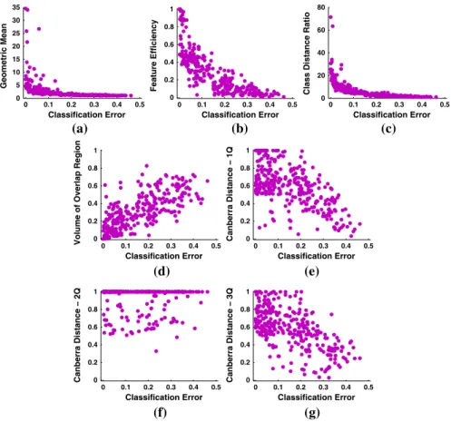
Figure7provides a visual description of the descriptive power of each feature. The figure shows scatter plots where each point corresponds to a single problem p2 Q0, the x-axis is a particular feature (SD, FE, CDR, VOR, 1, 2 and CD-3) and the y-axis is the associated CEl. The caption of Fig. 7 also gives the Pearson’s correlation coefficientq. It is evident that all of the chosen features are correlated with PGPC performance, in particular FE, VOR, CDR, CD-1 and CD-3 show the highest correlation.

4.5 Supervised learning of PEP models

It is now possible to pose a symbolic regression problem using the set T¼ fðbi;CEliÞg withi¼1;. . .;jQ

0_j_{, where the goal is to evolve a model}_K _that

(14)

linear models [17, 34, 57–60], but [57, 59, 60] showed that non-linear models evolved with GP achieved higher prediction accuracy.

Therefore, in this work we use a tree-based GP, configured with the parameters given in Table2. Three versions of the problem are posed, each with a different terminal set defined as subsets of all extracted features (4F, 5F, 7F) as specified in Table3. Set 4F uses the features with the four highest correlation coefficients (FE, CDR, VOR and CD-1), set 5F uses the features with the five highest correlation coefficients (SD, FE, CDR, VOR and CD-1), and 7F uses all of the seven features. The function set is defined asF¼ þn ;;; =;pﬃﬃ;sin;cos;log;xy;j j;ifo. Finally the fitness function is computed by the root mean squared error (RMSE) between the predicted CE and the true CEli, given by

fðKÞ ¼

ffiffiffiffiffiffiffiffiffiffiffiffiffiffiffiffiffiffiffiffiffiffiffiffiffiffiffiffiffiffiffiffiffiffiffiffiffiffiffiffiffiffiffiffi Pn

i¼1ðKðbiÞ CEliÞ 2 n s : ð8Þ 0 0.1 0.2 0.3 0.4 0.5 0 5 10 15 20 25 30 35 Classification Error Geometric Mean (a) (b) (d) (e) (f) (g) (c) 0 0.1 0.2 0.3 0.4 0.5 0 0.2 0.4 0.6 0.8 1 Classification Error Feature Efficiency 0 0.1 0.2 0.3 0.4 0.5 0 20 40 60 80 Classification Error

Class Distance Ratio

0 0.1 0.2 0.3 0.4 0.5 0 0.2 0.4 0.6 0.8 1 Classification Error

Volume of Overlap Region 00 0.1 0.2 0.3 0.4 0.5

0.2 0.4 0.6 0.8 1 Classification Error Canberra Distance − 1Q 0 0.1 0.2 0.3 0.4 0.5 0 0.2 0.4 0.6 0.8 1 Classification Error Canberra Distance − 2Q 0 0.1 0.2 0.3 0.4 0.5 0 0.2 0.4 0.6 0.8 1 Classification Error Canberra Distance − 3Q

Fig. 7 Scatter plots show the relationship between the CEl(x-axis) and each descriptive feature (y-axis)

for all problemsp2 Q0_{, where}_q_{specifies Pearson’s correlation coefficient.}_a_SD:_q_¼₀_:_42,_b_FE:

q¼ 0:78,cCDR:q¼ 0:62,dVOR:q¼ 0:72,eCD-1:q¼ 0:62,fCD-2:q¼ 0:03 andg

(15)

4.6 Testing the PEP models

For each version of the symbolic regression problem defined above (with different feature sets), we performed 100 runs using two different test scenarios: (1) train and test the PEP models using only synthetic problems; and (2) train with synthetic problems and test with real-world problems. In the first scenario, we use 70 % of the problems for training and the rest for testing, generating a random partition of the set of problemsQ0for each run. This is the simplest scenario, since both the training and testing problems are generated in the same manner. In the second scenario, we test the PEP models trained with synthetic problems and evaluate their predictions on many real-world datasets, a more challenging scenario since the real-world problems have high dimensional data, imbalanced classes and different data distributions.

4.6.1 Testing on synthetic classification problems

Table4summarizes the performance of the evolved PEPs, showing the median of the RMSE of the best solution found in each run for the training and testing sets, as well as the RMSE and Pearson’s correlation coefficientqof the best solution found. The table presents three rows of results, one for each feature set (PEP-4F, PEP-5F and PEP-7F). The numerical results are encouraging, suggesting that the PEP models can accurately predict PGPC performance. Moreover, there is a very small difference between training and testing performance, suggesting that the PEP models are not overfitted.

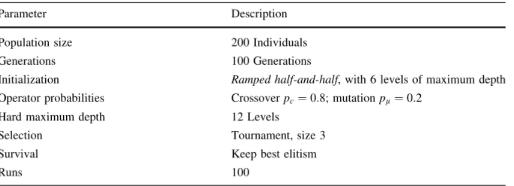
Table 2 Parameters for the GP used to derive PEP models for PGPC algorithm

Parameter Description

Population size 200 Individuals

Generations 100 Generations

Initialization Ramped half-and-half, with 6 levels of maximum depth

Operator probabilities Crossoverpc¼0:8; mutationpl¼0:2

Hard maximum depth 12 Levels

Selection Tournament, size 3

Survival Keep best elitism

Runs 100

Table 3 Three different features sets used as terminal elements for the symbolic regression GP algorithm

Feature vectorb

4F FE, CDR, VOR and CD-1

5F SD, FE, CDR, VOR and CD-1

(16)

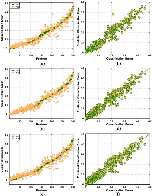
Figure8shows plots in three rows, where in each row we plot each feature set (PEP-4F, PEP-5F and PEP-7F). The plots on the left-hand side column show the PCE of the best PEP model and the true CElfor all synthetic problems, specifying the RMSE in the caption. The plots on the right-hand side column show the CEl and PCE as scatter plots, specifying the Pearson’s correlation coefficientq in the caption. The evolved PEPs produce accurate predictions with all feature sets. 4.6.2 Testing on real-world classification problems

This section presents the results of testing the best evolved PEPs to predict the testing error of PGPC on real-world problems. To this end, 22 real-world datasets are chosen from the University of California Irvine (UCI) machine learning repository [31], summarized in Table5. Since our PEPs only consider binary classification, we use these datasets to build 40 binary classification problems. The problems are summarized in Table6, specifying the name of the dataset and the classes used to define each problem, the number of total samples and the imbalance percentage of each problem computed asab_c where a and b are respectively the number of samples in the minority and majority class, andcis the total number of samples. Notice that the synthetic problems used to train the PEPs are completely balanced and relatively small problems in terms of number of samples, while the real-world problems are considerably more varied. In particular, considering class imbalance Fig.9 shows an histogram of the number of problems with different amounts of imbalance percentage.

Before testing the evolved PEP models, we compute the CElachieved by PGPC using 30 independent runs. PGPC performance is summarized in Fig.10, showing: (a) the CElfor each problem and (b) the histogram over CEl. Figures11presents scatter plots of each descriptive feature (x-axis) and the CEl (y-axis) of each problem, specifying the corresponding Pearson’s correlation coefficient q in the caption. The figures show that the best correlated features with CElare FE and CD-1, respectively withqvalues of-0.73 and-0.71. The rest of the features do not show particularly good correlation values, with SD clearly being the worst.

These results are different to what was observed on the synthetic problems. While VOR, CDR and CD-3 showed absolute correlation values above 0.6 on synthetic datasets, they were all below 0.44 on the real-world problems. This difference was particularly marked for SD, on synthetic problems the correlation

Table 4 Prediction performance of the evolved PEPs applied on the synthetic problems using each

feature set (4F, 5F and 7F, see Table3)

Median training RMSE Median testing RMSE Best RMSE Best correlation

PEP-4F 0.0320 0.0375 0.0318 0.9634

PEP-5F 0.0317 0.0362 0.0295 0.9688

PEP-7F 0.0326 0.0364 0.0317 0.9636

Performance is given based on the RMSE and Pearson’s correlation coefficient, with bold indicating the best performance

(17)

50 100 150 200 250 300 0 0.1 0.2 0.3 0.4 0.5 Classification Error Problem CEµ PCE 0 0.1 0.2 0.3 0.4 0.5 0 0.1 0.2 0.3 0.4 0.5 Classification Errror

Predicted Classification Error

(a) (b)

(c) (d)

(e) (f)

Fig. 8 Figures show for synthetic problems, the performance prediction of the best PEP models evolved

with the different feature set, each row belongs to each feature set: PEP-4F (top), PEP-5F (middle) and

PEP-7F (bottom).Plots on the left-hand side columnshow the PCE of the best solution and the known

CEl. The right-hand side column show scatter plots of the PCE and the CEl. a PEP-4F:

RMSE=0.0318, b PEP-4F: q¼0:9634, c PEP-5F: RMSE=0.0295, d PEP-5F: q¼0:9688, e

(18)

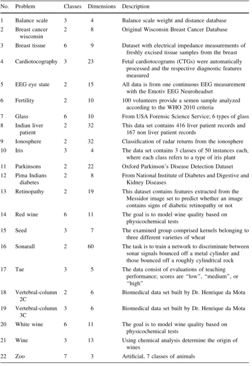
Table 5 Real-world datasets from the UCI machine learning repository used in this work

No. Problem Classes Dimensions Description

1 Balance scale 3 4 Balance scale weight and distance database

2 Breast cancer

wisconsin

2 8 Original Wisconsin Breast Cancer Database

3 Breast tissue 6 9 Dataset with electrical impedance measurements of

freshly excised tissue samples from the breast

4 Cardiotocography 3 23 Fetal cardiotocograms (CTGs) were automatically

processed and the respective diagnostic features measured

5 EEG eye state 2 15 All data is from one continuous EEG measurement

with the Emotiv EEG Neuroheadset

6 Fertility 2 10 100 volunteers provide a semen sample analyzed

according to the WHO 2010 criteria

7 Glass 6 10 From USA Forensic Science Service; 6 types of glass

8 Indian liver

patient

2 32 This data set contains 416 liver patient records and

167 non liver patient records

9 Ionosphere 2 32 Classification of radar returns from the ionosphere

10 Iris 3 4 The data set contains 3 classes of 50 instances each,

where each class refers to a type of iris plant

11 Parkinsons 2 22 Oxford Parkinson’s Disease Detection Dataset

12 Pima Indians

diabetes

2 8 From National Institute of Diabetes and Digestive and

Kidney Diseases

13 Retinopathy 2 19 This dataset contains features extracted from the

Messidor image set to predict whether an image contains signs of diabetic retinopathy or not

14 Red wine 6 11 The goal is to model wine quality based on

physicochemical tests

15 Seed 3 7 The examined group comprised kernels belonging to

three different varieties of wheat

16 Sonarall 2 60 The task is to train a network to discriminate between

sonar signals bounced off a metal cylinder and those bounced off a roughly cylindrical rock

17 Tae 3 5 The data consist of evaluations of teaching

performance; scores are ‘‘low’’, ‘‘medium’’, or ‘‘high’’

18 Vertebral-column

2C

2 6 Biomedical data set built by Dr. Henrique da Mota

19 Vertebral-column

3C

3 6 Biomedical data set built by Dr. Henrique da Mota

20 White wine 6 11 The goal is to model wine quality based on

physicochemical tests

21 Wine 3 13 Using chemical analysis determine the origin of

wines

(19)

Table 6 The 40 real-world binary classification problems based on the UCI datasets

No. Problem Classes Instances Imbalance %

1 Balance scale 1–3 576 0

2 Breast cancer wisconsin 1–2 699 31

3 Breast tissue 1–2 36 17 4 Breast tissue 1–3 39 8 5 Breast tissue 1–4 37 14 6 Breast tissue 2–3 33 9 7 Breast tissue 2–4 31 3 8 Breast tissue 3–4 34 6 9 Cardiotocography 1–2 1950 70 10 Cardiotocography 1–3 1831 81 11 Cardiotocography 2–3 471 26

12 EEG eye state 1–2 8388 17

13 Fertility 1–2 100 76

14 Glass 1–2 146 4

15 Glass 1–6 99 41

16 Glass 2–6 105 45

17 Indian liver patient 1–2 579 43

18 Ionosphere 1–2 351 28

19 Iris 1–2 100 0

20 Iris 1–3 100 0

21 Iris 2–3 100 0

22 Parkinsons 1–2 195 51

23 Pima indians diabetes 1–2 768 30

24 Red wine 5–6 1319 3 25 Retinopathy 1–2 1151 6 26 Seeds 1–2 140 0 27 Seeds 1–3 140 0 28 Seeds 2–3 140 0 29 Sonarall 1–2 208 7 30 Tae 1–2 99 1 31 Tae 1–3 101 3 32 Tae 2–3 102 2 33 Vertebral column 2C 1–2 310 35 34 Vertebral column 3C 1–2 210 43 35 Vertebral column 3C 1–3 160 25 36 Vertebral column 3C 2–3 250 20 37 White wine 5–6 3655 20 38 Wine 1–2 130 9 39 Wine 1–3 107 10 40 Zoo 1–2 61 34

(20)

coefficient was-0.42 but on real-world problems it is 0.09. In fact, only FE and CD-1 showed a good correlation on both sets.

Table7 summarizes the performance of the evolved PEPs applied on the real-world problems, showing the median of the RMSE of the best solution found, as well as the RMSE and Pearson’s correlation coefficientqof the best solution. The table presents three rows of results, one for each feature set (PEP-4F, PEP-5F and PEP-7F). In this case, the best performance is achieved by PEP-4F, which was unexpected. However, if we contrast the results with those achieved on the set of synthetic problems, shown in Table4, a performance drop-off is evident, based on both median and best performance.

Figure12shows three rows of plots, one for each feature set (PEP-4F, PEP-5F and PEP-7F). The figures on the left-hand side column show the PCE of the best PEP model and the true CElfor all real-world problems, specifying the RMSE. The

0 20 40 60 80 100 0 4 8 12 16 Imbalance Percentage Frecuency IMBALANCED PROBLEMS 1. The PEP models were trained

with balanced problems. 2. The real-world test problems

show a varied amount of imbal-anced cases.

Fig. 9 Histogram of imbalance percentage for the 40 real-world classification problems

5 10 15 20 25 30 35 40 0 0.1 0.2 0.3 0.4 0.5 Classification Error Problem (a) 0 0.15 0.3 0.45 0 5 10 15 20 25 Classification Error Frecuency (b)

Fig. 10 Performance of PGPC on the 40 real-world classification problems; whereashows the CElfor

(21)

figures on the right-hand side column show the CEl and PCE as scatter plots, specifying the Pearson’s correlation coefficientq. Again, these figures reveal that the evolved PEP models provide less accurate prediction on real-world problems.

0 0.1 0.2 0.3 0.4 0.5 0 10 20 30 40 50 Classification Error Geometric Mean 0 0.1 0.2 0.3 0.4 0.5 0 0.2 0.4 0.6 0.8 1 Classification Error Feature Efficiency 0 0.1 0.2 0.3 0.4 0.5 0 50 100 150 Classification Error

Class Distance Ratio

0 0.1 0.2 0.3 0.4 0.5 0 0.2 0.4 0.6 0.8 1 Classification Error

Volume of Overlap Region 0₀ _0.1 _0.2 _0.3 _0.4 _0.5

0.2 0.4 0.6 0.8 1 Classification Error Canberra Distance − 1Q 0 0.1 0.2 0.3 0.4 0.5 0 0.2 0.4 0.6 0.8 1 Classification Error Canberra Distance − 2Q 0 0.1 0.2 0.3 0.4 0.5 0 0.2 0.4 0.6 0.8 1 Classification Error Canberra Distance − 3Q (a) (b) (d) (e) (f) (g) (c)

Fig. 11 Scatter plots show for the real-world problems the relationship between the CEl(x-axis) and

each descriptive feature (y-axis).a SD: q¼0:09, b FE: q¼ 0:73, c CDR: q¼ 0:40, dVOR:

q¼0:43,eCD-1:q¼ 0:71,fCD-2:q¼ 0:46 andgCD-3:q¼ 0:30

Table 7 Prediction performance of the evolved PEPs applied on the real-world problems using each

feature set (4F, 5F and 7F, see Table3)

Median RMSE Best RMSE Best correlation

PEP-4F 0.1522 0.0828 0.8634

PEP-5F 0.1583 0.0929 0.8823

PEP-7F 0.1676 0.0930 0.8046

Performance is given based on the RMSE and Pearson’s correlation coefficient, with bold indicating the best performance

(22)

5 10 15 20 25 30 35 40 0 0.1 0.2 0.3 0.4 0.5 Classification Error Problem CEµ PCE 0 0.1 0.2 0.3 0.4 0.5 0 0.1 0.2 0.3 0.4 0.5 Classification Errror

(a) (b)

(c) (d)

(e) (f)

Fig. 12 Figures show for real-world problems, the performance prediction of the best PEP models

evolved with the different feature set, each row belongs to each feature set: PEP-4F (top), PEP-5F

(middle) and PEP-7F (bottom).Plots on the left-hand side columnshows the PCE of the best solution and

the known CEl. Theright-hand side columnshows scatter plots of the PCE and the CEl.aPEP-4F:

RMSE=0.0828,bPEP-4F:q=0.8634,cPEP-5F: RMSE=0.0929,dPEP-5F: RMSE=0.8823,

(23)

5 SPEP: specialist predictors of expected performance

The above results are encouraging, but for a real-world application even small improvements in the quality of the predictions could have non-negligible effects. Therefore, in this section we propose an ensemble approach using several PEP models, each one referred to as an SPEP. We propose an ensemble approach for two main reasons. First, previous works suggest that ensemble-based modeling can improve performance in a variety of scenarios [7, 76]. Second, an ensemble approach allows us to obtain two types of predictions, a numerical prediction of expected performance and a categorical or fuzzy prediction based on the chosen ensemble component used to compute the final prediction. The proposal is depicted in Fig.13, an extension of the basic PEP approach shown in Fig.1. However, in the SPEP approach before computing the PCE for a given problem, each problem is classified into a specific group using its corresponding feature vectorb. Each group is associated to a particular SPEP in the ensemble, hence if a problem is classified into the ith group then the ith SPEP is used to compute the predicted PGPC performance on the test set.

To implement this approach, several design choices must be specified. First, how to define a meaningful grouping of problems. Second, train SPEPs that are specialized for each group in order to build the ensemble. Third, chose the correct SPEP for a particular problem by determining its group membership. Each of these issues are discussed next.

5.1 Grouping problems based on PGPC performance and training SPEPs The proposal is to group problems based on the performance of PGPC given by CEl. This can be seem as a categorical prediction, where problems are grouped into general groups of different difficulty; e.g. easy and hard problems. In particular, we propose two different groupings based on CEl, using either two or three groups as shown in Fig.14. The groups were chosen in such a way that the number of (synthetic) problems in each group would be approximately the same, in this way posing a balanced classification task for the SPEP approach. Figure14shows the

Fig. 13 Block diagram shows the proposed SPEP approach. The proposed approach is an extension of

the basic PEP approach of Fig.1, with the additional ensemble approach, where problems are first

classified into prespecified groups and based on this a corresponding specialized morel (SPEP) is chosen to compute the PCE of PGPC on the test set

(24)

ranges of PGPC performance for each group and the number of synthetic problems (Fig.14a) and real-world problems (Fig.14b) that fall within each group. The plots on the top divide the problems into two groups, while the plots on the bottom divide the problems into three. Finally, for clarity, since the two group division requires two SPEPs, we refer to a solution for this task as an Ensemble-2, while a solution for the three group task is referred to as an Ensemble-3.

For each group an SPEP is trained using the same strategy described in the previous section for PEPs. Except that instead of using all of the synthetic problems, each SPEP is trained using the subset of synthetic problems from the corresponding group, as depicted in Fig.14. Since we are interested in presenting the best possible prediction of PGPC performance on real-world problems, we must select the best predictive models. Therefore, the testing phase is performed using two subsets of the real-world problems, one for validation and other for testing.

5.2 SPEP selection

As depicted in Fig.13, in order to choose an SPEP we must first classify each problem to its corresponding group. This is a straightforward classification task, solved using each problem’s feature vector b as the decision variables. Several classification algorithms are tested [5], namely:

1. Euclidean distance classifier (EDC). 2. Mahalanobis distance classifier (MDC). 3. Naive Bayes classifier (NBC).

4. Support vector machine (SVM), with Gaussian radial basis function kernel and a default scaling factor of 1.

5. K-Nearest Neighbor (KNN), usingK¼5 neighbors. 6. Treebagger Classifier (TBC), using three trees.

7. Probabilistic Genetic Programming Classifier (PGPC), parameters on Table1. Moreover, the classification task is posed using different subsets of the features inb as previously described in Table3. We apply all classifiers using all subsets of features on both the two-group and three-group classification tasks.

(a) (b)

Fig. 14 The proposed groupings of classification problems used with the SPEP approach, showing the ranges of PGPC performance and the number of problems in each group

(25)

As done for the SPEP models, in all cases the complete set of synthetic problems

Q0is used to train the classifiers. The testing phase is performed with two sets, 10 % of the real-world problems are used as a validation set while the remaining 90 % of real-world problems are used for testing. After performing 100 independent runs, the best solution is chosen based on its validation set performance, and methods are compared based on the performance on the testing set. If several solutions achieve the best validation set performance, than the final solution used in the ensemble is randomly chosen.

5.3 Evaluation of SPEP ensembles

This section presents the performance of the evolved SPEP models, and the performance of the complete ensembles, using both the true problem groups (an oracle approach, where the correct SPEP is always chosen) and the predicted group by the best classifier (a more realistic testing scenario).

5.3.1 Ensemble-2 solutions

To visualize the underlying difficulty of choosing the correct SPEP for a given problem (i.e., determining the group to which it belongs to) Fig.15 presents a parallel coordinate plot dividing the problems into two groups, where each coordinate is given by a feature inb. Plots are shown for synthetic (Fig.15a) and real-world problems (Fig.15b). The plots on the left show a single line for each problem, while the plots on the right show the median values for each group. For clarity in the parallel plots, the features SD and CDR were rescaled to values between [0, 1].

Table8 summarizes the performance of the best SPEP models used to build the Ensemble-2 solution. The first columns specifies the feature subset used fromb. The second column specifies the evaluated SPEP, SPEP-1 was trained with synthetic problems from the first group while SPEP-2 was trained with problems from the second group. The training RMSE is given in column 3. Every SPEP was tested on real-world problems from both groups, to illustrate the performance difference and specialization of each model; this is specified in the forth column. The final column gives the testing RMSE on each group.

The results show that the SPEP models are specialized to their groups, achieving error values below 0.1 when tested using problems from their groups, while performing worse when tested on problems from the other group. In general, performance on testing set is good, particularly if we compare with the results achieved by the PEP models from the preceding section. Finally, performance is similar for all feature sets when considering testing performance, with the best performance on Group 1 achieved by using the set 4F and the best performance on Group 2 with set 5F.

The results in Table 8 represent the best possible performance if the correct problem group is chosen, but also confirm that if the correct group is not chosen than prediction accuracy can decline. Table9summarizes the performance of all of

(26)

SD FE CDR VOR CD−1 CD−2 CD−3 0 0.1 0.2 0.3 0.4 0.5 0.6 0.7 0.8 0.9 1 Feature Value Group 1 Group 2 SD FE CDR VOR CD−1 CD−2 CD−3 0 0.1 0.2 0.3 0.4 0.5 0.6 0.7 0.8 0.9 1 Feature Value Group 1 Group 2 SD FE CDR VOR CD−1 CD−2 CD−3 0 0.1 0.2 0.3 0.4 0.5 0.6 0.7 0.8 0.9 1 Feature Value Group 1 Group 2 SD FE CDR VOR CD−1 CD−2 CD−3 0 0.1 0.2 0.3 0.4 0.5 0.6 0.7 0.8 0.9 1 Feature Value Group 1 Group 2 (a) (b)

Fig. 15 Parallel coordinate plots dividing the problems into two groups, where each coordinate is given

by a feature inb. Plots are shown for synthetic (a) and real-world problems (b). Theplots on the leftshow

a single line for each problem, while theplots on the rightshow the median values for each group

Table 8 RMSE of the best evolved SPEP models, using different feature sets (first column)

Performance is given based on training and testing set. Moreover, each

SPEP-icorresponds to theith problem

group but is tested on both problem groups, as specified in the fourth column. Bold indicates the best performance on each group

SPEP Training Testing group Testing

4F SPEP-1 0.0201 1 0.0315 2 0.2470 SPEP-2 0.0341 1 0.1445 2 0.0919 5F SPEP-1 0.0195 1 0.0380 2 0.1819 SPEP-2 0.0380 1 0.1119 2 0.0832 7F SPEP-1 0.0212 1 0.0469 2 0.2096 SPEP-2 0.0332 1 0.1586 2 0.1014

(27)

the tested classifiers for the two-group case, showing the median classification error achieved on the training and testing sets. On these tests, PGPC achieves the best performance based on test error.

Table10shows the performance of the best classifier obtained from each method and chosen based on the validation set. In this table performance is given using all real-world problems. Again, PGPC clearly outperforms all other variants, with the best performance achieved using feature set 7F with a classification error of 0.0250. It is now possible to evaluate the performance of the complete Ensemble-2 solutions, using the best evolved SPEPs and the best classifier. These results are summarized in Table11, specifying the RMSE and Pearson’s correlation coefficient when evaluated on the synthetic and real-world problem sets. These tests show that the Ensemble-2 solutions can achieve low predictive error and a high correlation with the true PGPC performance, for both synthetic and real-world problems. In particular, using feature set 5F correlation on synthetic problems is close to unity, while performance on the real-world problems show the lowest error and approximately 0.9 correlation.

Focusing on the real-world problems, Fig.16summarizes the performance of the Ensemble-2 predictors using each feature set (each row of the figure). The column on the left-hand side shows plots of the ground truth CEl of each problem

Table 9 Performance on the SPEP selection problem for all tested classifiers, showing the median classification error from 100 independent runs

Algorithm EDC MDC NBC SVM KNN TBC PGPC 4F Training 0.1533 0.0567 0.0200 0.0233 0.0133 0.0067 0.0100 Testing 0.2500 0.1389 0.1111 0.1111 0.1389 0.1111 0.0833 5F Training 0.1533 0.0567 0.0200 0.0200 0.0200 0.0067 0.0100 Testing 0.2778 0.1389 0.1389 0.1389 0.1667 0.1389 0.1111 7F Training 0.1533 0.0467 0.0200 0.0033 0.0200 0.0067 0.0100 Testing 0.2778 0.1389 0.1389 0.2500 0.1667 0.1111 0.0972

The performance is given on the training and testing sets Bold text indicates the best performance on each feature set

Table 10 Performance on the SPEP selection problem for all tested classifiers, showing the classification error of the best solution found, evaluated over all real-world problems, with bold indicating the best performance on each feature set

Feature set EDC MDC NBC SVM KNN TBC PGPC

4F 0.2500 0.1250 0.1000 0.1000 0.1250 0.1250 0.0500

5F 0.2750 0.1250 0.1250 0.1250 0.1500 0.1250 0.1000

(28)

(triangles) and the Ensemble-2 PCE. These plots show three types of PCE: (1) correctly classified problems for which the appropriate SPEP was selected (CC-PCE); (2) misclassified problems for which an incorrect SPEP was selected (MC-PCE); and (3) for the misclassified problems the oracle SPEP prediction (O-PCE), which is the PCE produced by the correct SPEP. The column on the right-hand side of Fig.16 presents scatter plots of the true CEl and the PCE, using the same notation.

These plots provide a graphical confirmation of the quality of the performance prediction. It is important to highlight the impact of a misclassified problem, shown as a black circle, compared to the prediction on the same problem if the correct SPEP had been chosen (O-PCE). For all problems for which the correct SPEP was chosen the PCE is highly correlated with the ground truth with only marginal differences in most cases.

5.3.2 Ensemble-3 solutions

Figure 17 presents a parallel coordinate plot dividing the problems into three groups, where each coordinate is given by a feature in b. Plots are shown for synthetic (Fig.17a) and real-world problems (Fig.17b). The plots on the left show a single line for each problem, while the plots on the right show the median values for each group. For clarity, features SD and CDR were rescaled to values between [0, 1].

Table12summarizes the performance of the best SPEP models used to build the Ensemble-3 solution. The first column, from left to right, specifies the feature subset used fromb. The second column specifies the evaluated SPEP, SPEP-1 was trained with synthetic problems from the first group, SPEP-2 with problems from the second group and SPEP-3 with problems from the third group. The third column shows the training RMSE, the fourth column shows the testing group and the final columns shows the testing RMSE.

Again, the results show that the SPEP models are specialized to their respective groups. Performance on the testing set is better than the simple PEP models, but worse than the Ensemble-2 solution presented before. All feature sets produce similar performance on testing set problems, with the best performance on Group 1

Table 11 Ensemble-2 prediction accuracy using each feature set (4F, 5F and 7F), using the best evolved SPEPs and the best classifiers with each feature set

Feature set Synthetic Real-world

RMSE Correlation RMSE Correlation

4F 0.0284 0.9709 0.0818 0.8717

5F 0.0302 0.9984 0.0736 0.8981

7F 0.0276 0.9728 0.0897 0.8514

Performance is given based on the RMSE and Pearson’s correlation coefficient when evaluated on the

(29)

5 10 15 20 25 30 35 40 0 0.1 0.2 0.3 0.4 0.5 ClassificationError Problem CEµ MC−PCE CC−PCE O−PCE 0 0.1 0.2 0.3 0.4 0.5 0 0.1 0.2 0.3 0.4 0.5 Classification Errror

(a) (b)

(c) (d)

(e) (f)

Fig. 16 Performance prediction of the best Ensemble-2 solutions for each feature set: 4F (top), 5F (middle) and 7F (bottom). Theleft-hand side column of plotsshow the ground truth CElof each problem (triangles) and the corresponding PCE (circles). Theright-hand side columnshows scatter plots between

the CEland the corresponding PCE. The PCE is presented in three different cases: the PCE of a correctly

classified problem (CC-PCE,circle); the PCE of a misclassified problem (MC-PCE,dark circle); and the

oracle PCE of a misclassified problem using the correct SPEP (O-PCE,circle with a cross).a4F: RMSE

= 0.0818,b4F:q¼0:8717,c5F: RMSE = 0.0736,d5F:q¼0:8981,e7F: RMSE = 0.0897 andf7F:

(30)

and Group 2 achieved by using set 4F, and the best performance on Group 3 with set 5F.

The results summarized in Table12represent the best possible performance if the correct problem group is chosen, but also confirm that if the correct group is not chosen than prediction accuracy can decline. Table13summarizes the performance of all of the tested classifiers for the three-group case, showing the median classification error achieved on the training and testing sets. On these tests, TBC achieves the best median performance. Table14focuses on the performance of the best classifier evaluated over all real-world problems. Again, TBC outperforms all other variants, with the best performance achieved using feature set 5F with a classification error of 0.1750.

It is now possible to evaluate the performance of the complete Ensemble-3 solutions, using the best evolved SPEPs and the best classifier. These results are summarized in Table15, specifying the RMSE and Pearson’s correlation coefficient when evaluated on the synthetic (training) and real-world (validation and testing) problem sets. These tests show that the Ensemble-3 solutions can achieve low predictive error and a high correlation with the true PGPC performance, for both

SD FE CDR VOR CD−1 CD−2 CD−3 0 0.1 0.2 0.3 0.4 0.5 0.6 0.7 0.8 0.9 1 Feature Value Group 1 Group 2 Group 3 SD FE CDR VOR CD−1 CD−2 CD−3 0 0.1 0.2 0.3 0.4 0.5 0.6 0.7 0.8 0.9 1 Feature Value Group 1 Group 2 Group 3 SD FE CDR VOR CD−1 CD−2 CD−3 0 0.1 0.2 0.3 0.4 0.5 0.6 0.7 0.8 0.9 1 Feature Value Group 1 Group 2 Group 3 SD FE CDR VOR CD−1 CD−2 CD−3 0 0.1 0.2 0.3 0.4 0.5 0.6 0.7 0.8 0.9 1 Feature Value Group 1 Group 2 Group 3 (a) (b)

Fig. 17 Parallel coordinate plots dividing the problems into three groups, where each coordinate is given

by a feature inb. Plots are shown for synthetic (a) and real-world problems (b). Theplots on the leftshow

(31)

synthetic and real-world problems. In all feature sets the correlation on synthetic problems is above 0.97, while the best performance on the real-world problems is achieved using set 5F based on RMSE and set 7F based on correlation.

Focusing on the real-world problems, Fig.18summarizes the performance of the Ensemble-3 predictors using each feature set (each row of the figure). These plots illustrate the performance of the achieved prediction. As in the Ensemble-2 case, it is important to highlight the impact of misclassified problems (shown as a black circle) compared to the prediction on the same problem if the correct SPEP had been chosen (O-PCE). In this case we can see more misclassifications. The reason is evident in Fig.17, since Group 2 and Group 3 are not so easily differentiated. However, the impact of the misclassified problems is not as large as it is for the

Table 12 RMSE of the best evolved SPEP models, using different feature sets (first column)

Performance is given based on training and testing set. Moreover, each

SPEP-icorresponds to theith problem

group but is tested on all problem groups, as specified in column 4

Bold text indicates best performance on each group

SPEP Training Testing group Testing

4F SPEP3-1 0.0201 1 0.0315 2 0.1312 3 0.2767 SPEP3-2 0.0303 1 0.1883 2 0.0302 3 0.1459 SPEP3-3 0.0264 1 0.3955 2 0.1349 3 0.0532 5F SPEP3-1 0.0195 1 0.0380 2 0.2076 3 0.1602 SPEP3-2 0.0313 1 0.0931 2 0.0380 3 0.1245 SPEP3-3 0.0294 1 0.2691 2 0.1250 3 0.0525 7F SPEP3-1 0.0212 1 0.0469 2 0.1723 3 0.2391 SPEP3-2 0.0285 1 0.1096 2 0.0352 3 0.1719 SPEP3-3 0.0277 1 0.1339 2 0.1133 3 0.0531