SFB
823
Testing for change in
stochastic volatility with long
range dependence
Discussion Paper
Annika Betken, Rafal Kulik
Testing for change in stochastic volatility with long
range dependence
Annika Betken
∗Rafa l Kulik
†November 6, 2016
Abstract
In this paper we consider a change point problem for long memory stochastic volatility models. We show that the limiting behavior for the CUSUM test statistics may not be affected by long memory, unlike the Wilcoxon test statistic which is influenced by long range dependence. We compare our results to subordinated long memory Gaussian processes. Theoretical properties are accompanied by simulation studies.
1
Introduction
One of the most often observed phenomena in financial data is the fact that the log-returns of stock-market prices appear to be uncorrelated, whereas the absolute log-log-returns or squared log-returns tend to be correlated or even exhibit long-range dependence. An-other characteristic of financial time series is the existence of heavy tails in the sense that the marginal tail distribution behaves like a regularly varying function. Both of these fea-tures of empirical data can be covered by the so-called long memory stochastic volatility model (LMSV, in short), with its original version introduced in [7]. For this we assume that the data generating process {Xj, j ≥1} satisfies
Xj =σ(Yj)εj, j ≥1, (1)
where
• {εj, j ≥1} is an i.i.d. sequence with mean zero;
• {Yj, j ≥1} is a stationary, long-range dependent Gaussian process;
∗Ruhr-Universit¨at Bochum, Fakult¨at f¨ur Mathematik, [email protected]; Research supported by
the German National Academic Foundation and Collaborative Research Center SFB 823Statistical mod-elling of nonlinear dynamic processes.
• σ(·) is a non-negative measurable function, not equal to 0.
Note that within this model long memory results from the subordinated Gaussian sequence
{Yj, j ≥1}only. More precisely, we assume that {Yj, j ≥1}admits a linear representation
with respect to an i.i.d. Gaussian sequence {ηj, j ≥1} with E(η1) = 0, Var(η1) = 1, i.e.
Yj = ∞ X k=1 ckηj−k , j ≥0, (2) with P∞ k=1c2k = 1 and γY(k) = Cov(Yj, Yj+k) =k−DLγ(k),
where D∈(0,1) and Lγ is slowly varying at infinity. Also, we assume that
• {(εj, ηj), j ≥1} is a sequence of i.i.d. vectors.
The above set of assumptions we will call collectively LMSV model.
The tail behavior of the sequence {Xj, j ≥1}can be related to the tail behavior of εj
orσ(Yj) or both. Here we will specifically assume that
• random variables εj have a marginal distribution with regularly varying right tail,
i.e. ¯Fε(x) :=P(ε1 > x) =x−αL(x) for some α >0 and a slowly varying function L, such that the following tail balance condition holds:
lim x→∞ P(ε1 > x) P(|ε1|> x) =p= 1− lim x→∞ P(ε1 <−x) P(|ε1|> x) for some p∈(0,1]; • it holds Eσα+δ(Y0) <∞ for some δ >0.
Under these conditions, it follows by Breiman’s Lemma (see [17, Proposition 7.5]) that
P(X1 > x)∼E[σα(Y1)]P(ε1 > x), (3) i.e. the process {Xj, j ≥1}inherits the tail behavior from {εj, j ≥1}.
We would like to point out here that in the literature the usage of the term LMSV often presupposes that the sequences {Yj, j ≥1} and {εj, j ≥1} are independent. In this
paper we will consider a more general model: instead of claiming mutual independence of {Yj, j ≥ 1} and {εj, j ≥ 1}, we only assume that (ηj, εj) is a sequence of independent
random vectors. Especially, this implies that for a fixed index j the random variables εj
and Yj are independent whileYj may depend on{εi, i < j}. In many cases this version of
1.1
Change-point detection under long memory
One of the problems related to financial data is to detect change points in the behavior of the sequence {Xj, j ≥ 1}. Although the problem has been extensively studied for
independent random variables (see an excellent book [8]) or in case of weakly dependent data, the issue has not been fully resolved for time series with long memory. The researchers focused rather on justifying whether the observed long range dependence is real or is due to changes in weakly dependent sequences (so-called spurious long memory). See e.g. [3] and Section 7.9.1 of [2] for further references on the latter issue.
As for the testing changes in long memory sequences, one of the first paper seems to be [13], where the authors showed that long range dependence affects the asymptotic behavior of the CUSUM statistics for changes in the mean. For the general testing problem with a change in the marginal distribution under the alternative hypothesis, [12] consider Kol-mogorov - Smirnov type change-point tests and change-point estimators for long memory moving average processes. Under the assumption of converging change-point alternatives in LRD time series, the asymptotic behavior of Kolmogorov-Smirnov and Cram´er-von Mises type test statistics has also been investigated by [22]. Likewise, [9] show that the Wilcoxon test is always affected by long memory. In fact, in the case of Gaussian long memory data, the asymptotic relative efficiency of the Wilcoxon test and the CUSUM test is 1.
In case of long range dependence, the normalization and the limiting distribution of test statistics typically depend on unknown multiplicative factors or parameters related to the dependence structure of the data generating processes. To bypass estimation of these quantities, the concept of self-normalization has recently been applied to several testing procedures in change-point analysis: In [19] the authors define a self-normalized Kolmogorov-Smirnov test statistic that serves to identify changes in the mean of short range dependent time series. [18] adopted the same approach to define an alternative normalization for the CUSUM test; [4] considers a self-normalized version of the Wilcoxon change-point test proposed by [9].
We refer also to Section 7.9 of [2] for further results on change-point detection for long memory processes.
1.2
Change-point detection for LMSV
In this paper we study CUSUM and Wilcoxon tests for LMSV model and discuss particular cases of testing changes in the mean, in the variance and in the tail index. Of course, the variance and the tail index can be regarded as the mean of transformed random variables, but we observe different effects for each of the three quantities. In particular, the main findings of our paper are as follows:
A-1: CUSUM tests for change in the mean for the LMSV models is typically not affected by long memory (see Corollary 3.2 and Example 4.1). This is different than the findings in [13] for subordinated Gaussian processes;
A-2: Wilcoxon test for change in the mean for the LMSV models is typically affected by long memory (see again Corollary 3.2 and Example 4.1). This is in line with the findings for subordinated Gaussian processes
Hence, to test changes in the mean for the LMSV it is beneficial to use CUSUM test. B: CUSUM and Wilcoxon tests for change in the variance for the LMSV models are
typically affected by long memory; see Section4.2.
B: CUSUM and Wilcoxon tests for change in the tail index for the LMSV models are typically affected by long memory; see Section4.3
The paper is structured as follows. In Section 2 we collect some results on subordinated Gaussian processes. In Section 3 we discuss the change-point problem. In particular, we consider CUSUM test and Wilcoxon test. The former is a direct consequence of the existing results, while the latter requires a new theorem on the limiting behavior of empirical processes based on LMSV data. Section4is devoted to examples in case of testing changes in the mean, in the variance and in the tail. Since the test statistics and/or limiting distributions involve unknown quantities, self-normalization is considered in Section 5. In fact, in Section 6 we perform simulation studies and indicate that self-normalization provides robustness.
2
Preliminaries
2.1
Some properties of subordinated Gaussian sequences
The main tool for studying the asymptotic behavior of subordinated Gaussian sequences is the Hermite expansion. For a stationary, long-range dependent Gaussian process {Yj, j ≥
1} and a measurable function g such that E(g2(Y
1)) < ∞ the corresponding Hermite expansion is defined by g(Y1)−E (g(Y1)) = ∞ X q=m Jq(g) q! Hq(Y1), where Hq is the q-th Hermite polynomial,
Jq(g) = E (g(Y1)Hq(Y1))
and
m = inf{q≥1|Jq(g)6= 0} .
The integer m is called the Hermite rank of g and we refer to Jq(g) as the q-th Hermite
coefficient of g.
We will also consider the Hermite expansion of the function class
where Fg(Y1) denotes the distribution function of g(Y1). For fixedx we have 1{g(Y1)≤x}−Fg(Y1)(x) = ∞ X q=m Jq(g;x) q! Hq(Y1) with Jq(g;x) = E 1{g(Y1)≤x}Hq(Y1) .
The Hermite rank corresponding to this function class is defined by m= infxm(x), where
m(x) denotes the Hermite rank of 1{g(Y1)≤x}−Fg(Y1)(x). See [2].
The asymptotic behavior of partial sums of subordinated Gaussian sequences is char-acterized in [21]. Due to the functional non-central limit theorem in that paper,
1 dn,m bntc X j=1 g(Yj)⇒ Jm(g) m! Zm(t), 0≤t≤1, (4) where d2n,m = Var n X j=1 Hm(Yj) ! ∼cmn2−mDLm(n), cm = 2m! (1−Dm)(2−Dm),
Zm(t), 0≤t ≤1, is an m-th order Hermite process and the convergence holds inD([0,1]),
the space of functions that are right continuous with left limits. In fact the limiting behavior in (4) is the same as that of the corresponding partial sums based on {Hm(Yj), j ≥1}:
Jm(g) 1 dn,m bntc X j=1 Hm(Yj)⇒ Jm(g) m! Zm(t), 0≤t≤1.
Moreover, the functional central limit theorem for the empirical processes was established in [10]. Specifically, sup −∞≤x≤∞ sup 0≤t≤1 d−n,m1 bntc Gbntc(x)−E Gbntc(x) −Jm(g;x) bntc X j=1 Hm(Yj) P −→0, (5) where Gl(x) = 1 l l X j=1 1{g(Yj)≤x}
is the empirical distribution function of the sequence {g(Yj), j ≥ 1} and P
−→ denotes
convergence in probability. Thus, the empirical process
d−n,m1 bntc
Gbntc(x)−E Gbntc(x) , x∈(−∞,∞), t∈[0,1],
converges in D([−∞,∞]×[0,1]) to Jm(g;x)Zm(t).
3
Change-point problem
Given the observations X1, . . . , Xn and a function ψ, we define ξj =ψ(Xj), j = 1, . . . , n,
and we consider the testing problem:
H0 : E(ξ1) =· · ·= E(ξn),
H1 :∃ k ∈ {1, . . . , n−1} such that E(ξ1) =· · ·= E(ξk)6= E(ξk+1) =· · ·= E(ξn).
We choose ψ according to the specific change-point problem considered. Possible choices include:
• ψ(x) = x in order to detect changes in the mean of the observations X1, . . . , Xn
(change in location);
• ψ(x) =x2 in order to detect changes in the variance of the observations X1, . . . , Xn
(change in volatility);
• ψ(x) = log(x2) or ψ(x) = log(|x|) in order to detect changes in the index α of heavy-tailed observations (change in the tail index).
It is obvious that ψ(x) = x and ψ(x) = x2 lead to testing a change in the mean and variance, respectively. The choice ψ(x) = log(|x|) requires an additional comment. We note that (3) describes only the asymptotic tail behavior of X1. For the purpose of this paper, we shall pretend that P (|X1|> x) = cαx−α, x > c, for some c > 0. Then the maximum likelihood estimator of (1/α), the reciprocal of the tail index, is
1 n n X j=1 log (|Xj|/c) . (6)
This estimator is used in the CUSUM test statistic. To resolve the problem of change-point in the tail index in full generality, we need to employ a completely different technique, based on the so-called tail empirical processes (see [15]). This will be done in a subsequent paper. In any case, the following test statistics may be applied in order to decide on the change-point problem (H0, H1):
• The CUSUM test rejects the hypothesis for large values of the test statistic Cn =
sup 0≤λ≤1 Cn(λ), where Cn(λ) = bnλc X j=1 ψ(Xj)− bnλc n n X j=1 ψ(Xj) . (7)
• The Wilcoxon test rejects the hypothesis for large values of the test statistic Wn = sup 0≤λ≤1 Wn(λ), where Wn(λ) = bnλc X i=1 n X j=bnλc+1 1{ψ(Xj)≤ψ(Xj)}− 1 2 . (8)
The goal of this paper is to obtain limiting distributions for the CUSUM and the Wilcoxon test statistic in case of time series that follow the LMSV model.
3.1
CUSUM Test for LMSV
In order to determine the asymptotic behavior of the CUSUM test statistic computed with respect to the observationsψ(X1), . . . , ψ(Xn), we have to consider the partial sum process Pbntc
j=1(ψ(Xj)−E (ψ(Xj))).
For the observationsX1, . . . , Xn that satisfy the LMSV model, the asymptotic behavior
of the partial sum process is described by Theorem 4.10 in [2] and hence is stated without the proof. In order to formulate the result, we introduce the following notation:
Fj =σ(εj, εj−1, . . . , ηj, ηj−1, . . .),
i.e. Fj denotes theσ-field generated by the random variablesεj, εj−1, . . . , ηj, ηj−1, . . .. Due to the construction εj is independent of Fj−1 and Yj is Fj−1-measurable.
Theorem 3.1. Assume that {Xj, j ≥ 1} follows the LMSV model. Furthermore, assume that E(ψ2(X
1)) < ∞. Define the function Ψ by Ψ(y) = E (ψ(σ(y)ε1)). Denote by m the
Hermite rank of Ψ and by Jm(Ψ) the corresponding Hermite coefficient.
1. If E(ψ(X1)| F0)6= 0 and mD <1, then 1 dn,m bntc X j=1 (ψ(Xj)−E(ψ(Xj))) ⇒ Jm(Ψ) m! Zm(t), t∈[0,1], in D([0,1]). 2. If E(ψ(X1)| F0) = 0, then 1 √ n bntc X j=1 ψ(Xj)⇒σB(t), t∈[0,1],
As the immediate consequence of Theorem 3.1 we obtain the asymptotic distribution for the CUSUM statistic.
Corollary 3.2. Under the assumptions of Theorem 3.1, 1. If E(ψ(X1)| F0)6= 0 and mD <1, then 1 dn,m sup 0≤λ≤1 Cn(λ)⇒ Jm(Ψ) m! 0sup≤t≤1 |Zm(t)−tZm(1)| . (9) 2. If E(ψ(X1)| F0) = 0 1 √ n0≤supλ≤1 Cn(λ)⇒ √ σ sup 0≤t≤1 |B(t)−tB(1)| ,
where B denotes a Brownian motion process and σ2 = E(ψ2(X
1)).
It is important to note that the Hermite rank of Ψ does not necessarily correspond to the Hermite rank of σ. See Section 4.
3.2
Wilcoxon test for LMSV
For subordinated Gaussian time series {g(Yj), j ≥ 1}, where {Yj, j ≥ 1} is a stationary
Gaussian LRD process and g is a measurable function, the asymptotic distribution of the Wilcoxon test statistic Wn is derived from the limiting behavior of the two-parameter
empirical process bntc X j=1 1{g(Yj)≤x}−Fg(Y1)(x) , x∈(−∞,∞), t ∈[0,1],
where Fg(Y1) denotes the distribution function of g(Y1); see [9].
In order to determine the asymptotic distribution of the Wilcoxon test statistic for the LMSV model, we need to establish an analogous result for the stochastic volatility process
{Xj, j ≥ 1}, i.e. our preliminary goal is to prove a limit theorem for the two-parameter
empirical process Gn(x, t) = bntc X j=1 1{ψ(Xj)≤x}−Fψ(X1)(x) ,
where now Fψ(X1) denotes the distribution function of ψ(X1) with X1 =σ(Y1)ε1. To state
the weak convergence, we introduce the following notation. Define Ψx(y) = P(ψ(yε1)≤x) .
Theorem 3.3. Assume that{Xj, j ≥1} follows the LMSV model. Moreover, assume that Z ∞
−∞ d
duP (ψ(uε1)≤x)du <∞. (10)
IfmD <1, wherem denotes the Hermite rank of the class1{σ(Y1)≤x}−Fσ(Y1)(x), x∈R ,
1 dn,m Gn(x, t)⇒ Jm(Ψx◦σ) m! Zm(t), (11) in D([−∞,∞]×[0,1]) .
The proof of this theorem is given in Section 3.3. At this moment we conclude the asymptotic distribution of the Wilcoxon statistics.
Corollary 3.4. Under the conditions of Theorem 3.3
1 ndn,m sup λ∈[0,1] Wn(λ)⇒ Z R Jm(Ψx◦σ)dFψ(X1)(x) 1 m!λsup∈[0,1] |Zm(λ)−λZm(1)| . Proof of Corollary 3.4. According to [9], the asymptotic distribution of the Wilcoxon test statistic can be concluded directly from the limit of the two-parameter empirical process if the sequence {Xj, j ≥ 1} is ergodic. Ergodicity is obvious since Xj can be represented
as a measurable function of the i.i.d. vectors {(ηj, εj), j ≥1}.
3.3
Proof of Theorem
3.3
To prove Theorem 3.3, we consider the following decomposition:
Gn(x, t) = bntc X j=1 1{ψ(Xj)≤x}−E 1{ψ(Xj)≤x}| Fj−1 + bntc X j=1 E 1{ψ(Xj)≤x}| Fj−1 −Fψ(X1)(x) =:Mn(x, t) +Rn(x, t).
It will be shown thatn−1/2M
n(x, t) =OP(1) uniformly inx, t, whiled−n,m1 Rn(x, t) converges
in distribution to the limit process in formula (11). Theorem 3.3 then follows because
√
n= o(dn,m).
Martingale part. For fixedxthe following lemma characterizes the asymptotic behavior of the martingale part Mn(x, t). We write
Mn(t) :=Mn(x, t) = bntc X j=1 ζj(x) with ζj(x) = 1{ψ(Xj)≤x}−E 1{ψ(Xj)≤x}| Fj−1 .
Lemma 3.5. Under the conditions of Theorem 3.3 we have
1
√
nMn(t)⇒β(x)B(t), t∈[0,1],
in D([0,1]), where B denotes a Brownian motion process and β2(x) = E(ζ2 1(x)). Proof. Define ζnj =n− 1 2ζj(x) =Xnj(x)−E(Xnj(x)| Fj−1) with Xnj(x) = n− 1 21{ψ(X
j)≤x}. In order to show convergence in D([0,1]), we apply the
functional martingale central limit theorem as stated in Theorem 18.2 of [6]. Therefore, we have to show that
bntc X j=1 E ζnj2 | Fj−1 ⇒β(x)t
for every t and that
lim n→∞ bntc X j=1 E ζnj2 1{|ζnj|≥} = 0
for everyt and >0 (Lindeberg condition). In order to show that the Lindeberg condition holds, it suffices to show that
lim n→∞ bntc X j=1 EXnj2 (x)1{|X nj(x)|≥2} = 0 (12)
due to Lemma 3.3 in [11]. As the indicator function is bounded, the above summands vanish for sufficiently large n and hence (12) follows.
Furthermore, the random variable E ζ2
j(x)| Fj−1
can be considered as a measurable function of the random variableYj and therefore as a function of εj−1, εj−2, . . .. As a result, E ζj2(x)| Fj−1
is an ergodic sequence and it follows by the ergodic theorem that 1 n bntc X j=1 E ζj2(x)| Fj−1 = bntc n 1 bntc bntc X j=1 E ζj2(x)| Fj−1 P −→tE(ζ12(x)) for every t.
The next lemma establishes tightness of the two-parameter process.
Lemma 3.6. Under the conditions of Theorem 3.3 we have
1
√
nMn(x, t) = OP(1)
in D([−∞,∞]×[0,1]).
Long memory part. Finally, we prove weak convergence of the long memory part
Rn(x, t).
Lemma 3.7. Under the conditions of Theorem 3.3,
1 dn,m Rn(x, t)⇒ Jm(Ψx◦σ) m! Zm(t), in D([−∞,∞]×[0,1]) .
Proof. Note that
E 1{ψ(Xj)≤x}| Fj−1
= E 1{ψ(σ(Yj)εj)≤x}| Fj−1
= Ψx(σ(Yj))
becauseYj isFj−1-measurable andεj is independent ofFj−1. Furthermore, E (Ψx(σ(Yj))) =
Fψ(X1)(x), the distribution function of ψ(X1) =ψ(σ(Y1)ε1). Hence,
Rn(x, t) = bntc X j=1 (Ψx(σ(Yj))−F(x)) =bntc Z ∞ −∞ Ψx(u)d Gbntc−EGbntc (u), where Gl(u) = 1 l l X j=1 1{σ(Yj)≤u}
is the empirical distribution function of the sequence{σ(Yj), j ≥1}. We have,
d−n,m1 Rn(x, t) =d−n,m1 bntc Z ∞ −∞ Ψx(u)d Gbntc−EGbntc (u) =− ( Z ∞ −∞ d duP (ψ(uε1)≤x)d −1 n,m bntc Gbntc(u)−EGbntc(u) −Jm(σ;u) m! bntc X j=1 Hm(Yj) du ) − ( Z ∞ −∞ d duP (ψ(uε1)≤x)d −1 n,m Jm(σ;u) m! bntc X j=1 Hm(Yj)du ) =:I1(x, t) +I2(x, t),
where m denotes the Hermite rank of the class1{σ(Y1)≤x}−Fσ(Y1)(x), x∈R and
Jm(σ;y) = E 1{σ(Y1)≤y}Hm(Y1)
Using the reduction principle (5) withg =σ and the integrability condition (10), we con-clude that the first summand converges to 0 in probability, uniformly inx, t. Furthermore,
I2(x, t) =− ( Z ∞ −∞ d duP (ψ(uε1)≤x)d −1 n,m Jm(σ;u) m! bntc X j=1 Hm(Yj)du ) =−d−n,m1 bntc X j=1 Hm(Yj) ( Z ∞ −∞ d duP(ψ(uε1)≤x) Jm(σ;u) m! du ) . We have d−n,m1 bntc X j=1 Hm(Yj)⇒Zm(t).
Moreover, integration by parts yields
Z ∞ −∞ d duP (ψ(uε1)≤x)Jm(σ;u)du = Z ∞ −∞ d duP(ψ(uε1)≤x) Z 1{σ(z)≤u}Hm(z)ϕ(z)dzdu = Z ∞ −∞ Hm(z)ϕ(z) Z d duP (ψ(uε1)≤x) 1{σ(z)≤u}dudz = Z ∞ −∞ Hm(z)ϕ(z) Z ∞ σ(z) d duP(ψ(uε1)≤x)dudz = lim u→∞P (ψ(uε1)≤x) Z ∞ −∞ Hm(z)ϕ(z)dz− Z ∞ −∞ P(ψ(σ(z)ε1)≤x)Hm(z)ϕ(z)dz =−Jm(Ψx◦σ).
4
Examples
4.1
Change in the mean
To test a change in the mean we choose ψ(x) =x.
CUSUM:Recall that the function Ψ in Theorem 3.1 is defined as Ψ(y) = E (ψ(σ(y)ε1)). In this case
E(ψ(X1)| F0) = σ(Y1) E(ε1) = 0.
• Long memory does not influence the asymptotic behavior of the CUSUM statistic for testing change in the mean.
Wilcoxon: Recall that Ψx(y) = P(ψ(yε1)≤x). Using the integration by parts and noting that (d/dz)ϕ(z) =−zϕ(z) we have J1(Ψx◦σ) = Z ∞ −∞ P (ψ(σ(z)ε1)≤x)zϕ(z)dz = Z ∞ −∞ d dzP (ψ(σ(z)ε1)≤x)ϕ(z)dz = Z ∞ −∞ d dzP ε1 ≤ x σ(z) ϕ(z)dz = Z ∞ −∞ 1 σ(z) 0 fε x σ(z) ϕ(z)dz ,
wherefεis the density ofε1(if it exists). Here, different scenarios are possible. Ifσ(y) =y2
then z → 1
σ(z)
fε(x/σ(z))0ϕ(z) is antisymmetric for any x and any choice of fε. Hence,
J1(Ψx◦σ) = 0 and one can calculate that the Hermite rank of Ψx◦σ is 2. Ifσ(y) = exp(y)
and e.g. ε1 is Pareto-distributed, i.e. for some α >0, c >0
fε(x) = ( αcα xα+1, x≥c 0, x < c ,. then, as a result, Z ∞ −∞ e−z αc α x exp(z) α+11{exp(xz)≥c}ϕ(z)dz =αcαx−(α+1) Z ∞ −∞ exp(zα)1{log(x c)≥z} ϕ(z)dz =αcαx−(α+1)√1 2π Z log(xc) −∞ exp(zα− 1 2z 2) | {z } >0 dz .
Hence, J1(Ψx◦σ)6= 0. In any case,
• Long memory influences the asymptotic behavior of the Wilcoxon statistic, unlike the CUSUM one.
4.2
Change in the variance
To test a change in the variance we choose ψ(x) =x2.
CUSUM:Recall again that the function Ψ in Theorem3.1is defined as Ψ(y) = E (ψ(σ(y)ε1)). Then
and hence long memory affects the limiting behavior of the CUSUM statistic. Moreover, Jm(Ψ) = E(ε21) Z σ2(z)Hm(z)ϕ(z)dz = E ε21 Jm(σ2),
i.e. the Hermite rank of Ψ equals the Hermite rank of σ2. If mD < 1 then the limiting behavior of the CUSUM statistic is described by (9). Hence,
• Long memory influences the asymptotic behavior of the CUSUM statistic for testing change in the variance.
Wilcoxon: Recall again that Ψx(y) = P(ψ(yε1)≤x). We have
J1(Ψx◦σ) = Z ∞ −∞ P(ψ(σ(z)ε1)≤x)zϕ(z)dz = Z ∞ −∞ d dzP(ψ(σ(z)ε1)≤x)ϕ(z)dz = Z ∞ −∞ d dzP ε21 ≤ x σ2(z) ϕ(z)dz = Z ∞ −∞ 1 σ2(z) 0 fε x σ2(z) ϕ(z)dz .
If σ(y) = exp(−y) then we are in the same situation as in case of testing the mean and hence J1(Ψx◦σ)6= 0. Hence,
• Long memory influences the asymptotic behavior of the Wilcoxon statistic for testing change in the variance.
4.3
Change in the tail index
To test a change in the tail index we choose ψ(x) = log(x2).
CUSUM:In this case
E(ψ(X1)| F0) = log(σ2(Y1)) + E(log(ε21))6= 0
and hence long memory affects the limiting distribution of the CUSUM statistic. Moreover,
Jm(Ψ) = 2 Z
log(σ(z))Hm(z)ϕ(z)dz = 2Jm(log◦σ),
so that the Hermite rank of Ψ equals the Hermite-rank ofh= log◦σ. We note further that in case of ψ(x) = log(x2) we have
1 dn,m bnλc X j=1 log Xj2−E log Xj2 = 2 dn,m bnλc X j=1 (logσ(Yj)−E logσ(Yj)) + √ n dn,m 1 √ n bnλc X j=1 log ε2j−E log ε2j.
The first summand converges to (Jm(log◦σ)/m!)Zm(λ) as a consequence of the functional
non-central limit theorem discussed in Section 2.1. The second term is oP(1) uniformly in
λ by Donsker’s theorem, if Var(logε2
1) < ∞. As a result, this observations is consistent with Corollary 3.2.
In summary
• Long memory influences the asymptotic behavior of the CUSUM statistic for testing change in the tail index.
5
Self-normalization
An application of the CUSUM test presupposes knowledge of the normalizing sequence
dn,m (if E(ψ(X1)| F0)6= 0) and of the coefficients Jm(Ψ) or σ that appear in the limit of
the test statistic. Usually, these quantities are unknown. In order to avoid estimation of the normalization and the unknown coefficients in the limit, we consider the self-normalized CUSUM test statistic with respect to the observations ξj = ψ(Xj), j = 1, . . . , n. For
0< τ1 < τ2 <1 it is defined by Tn(τ1, τ2) = sup k∈{bnτ1c,...,bnτ2c} |Gn(k)|, where Gn(k) = Pk j=1ξj− k n Pn j=1ξj n 1 n Pk t=1St2(1, k) + 1n Pn t=k+1St2(k+ 1, n) o12, with St(j, k) = t X h=j ξh−Z¯j,k , ¯ Zj,k = 1 k−j+ 1 k X t=j ξt.
The self-normalized CUSUM test rejects the hypothesis for large values of the test statistic
Tn(τ1, τ2). Note that the proportion of the data that is included in the calculation of the supremum is restricted by τ1 and τ2. A common choice is τ1 = 1−τ2 = 0.15; see [1].
In order to detect changes in the mean of (possibly) long-range dependent time series, a similar test statistic has been proposed by in [18]. For long memory stochastic volatility sequences the limit of the test statistic can be derived in the same way as in [18]. Under the assumptions of Theorem 3.1 (and if E(ψ(X1)| F0) 6= 0 and mD < 1), an application
of the continuous mapping theorem to the partial sum process d1 n Pbntc j=1(ψ(Xj)−Eψ(Xj)) yieldsTn(τ1, τ2) D −→ T(m, τ1, τ2), where T(m, τ1, τ2) = sup λ∈[τ1,τ2] |Zm(λ)−λZm(1)| n Rλ 0 V 2 m(r; 0, λ)dr+ R1 λ V 2 m(r;λ,1)dr o12 with Vm(r;r1, r2) =Zm(r)−Zm(r1)− r−r1 r2−r1 {Zm(r2)−Zm(r1)} for r∈[r1, r2], 0< r1 < r2 <1.
If E(ψ(X1)| F0) = 0, it follows by an application of the continuous mapping theorem to the partial sum process √1
n Pbntc j=1 ψ(Xj) thatTn(τ1, τ2) D −→ T(τ1, τ2), where T(τ1, τ2) = sup λ∈[τ1,τ2] |B(λ)−λB(1)| n Rλ 0 V2(r; 0, λ)dr+ R1 λ V2(r;λ,1)dr o12 with V(r;r1, r2) =B(r)−B(r1)− r−r1 r2−r1 {B(r2)−B(r1)}
for r ∈ [r1, r2], 0 < r1 < r2 < 1. Note that in this case the limit does not depend on any unknown parameters: for one thing the factor σ that appeared in the limit of the partial sum process is canceled out by self-normalization, for another thing the limit does neither depend on the Hermite rank m nor on the Hurst parameter H.
6
Simulations
6.1
Change in the mean
We will now investigate the finite sample performance of the CUSUM and Wilcoxon change-point test for detecting changes in the mean of LMSV time series{Xj, j ≥1}, i.e. we choose
ψ(x) =x for the test statistics Cn and Wn as described in Section 3.
For the simulations we make the following specifications:
Xj =σ(Yj)εj, j ≥0, (13)
where
• {Yj, j ≥1} is a fractional Gaussian noise generated by the function fgnSim (fArma
package inR) with the Hurst parameter H (note that H and the memory parameter
D are linked by H = 1−D/2);
• σ(y) = exp(y).
In order to determine the finite sample performance under the alternative, we simulate time series with a change-point of height h after τ percent of the data, i.e. we consider random variables Xj, j = 1, . . . , n with expected value µj, j = 1. . . , n such that µj = µ
for j = 1, . . . ,bnτc while µj =µ+hfor j =bnτc+ 1, . . . , n.
Recall that the function Ψ in Theorem 3.1 is defined as Ψ(y) = E (ψ(σ(y)ε1)). In this case E(ψ(X1)| F0) = σ(Y1) E(ε1) = 0. Due to Corollary 3.2 1 √ n0≤supλ≤1 Cn(λ)⇒ √ σ sup 0≤t≤1 |B(t)−tB(1)| ,
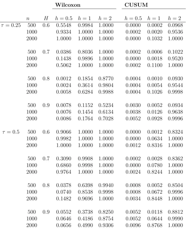
where σ2 = E(ψ2(X1)) = E(ε21exp(2Y1)) = E(exp(2Y1)) = exp(2). Hence, we expect long memory in the data not to influence the asymptotic behavior of the CUSUM statistic for testing change in the mean. In fact, our simulations confirm that the power of the CUSUM point test does not change significantly when different values forHare considered; see Table
1.
In order to compute the asymptotic distribution of the Wilcoxon test in the above situation, note that
J1(Ψx◦σ) = Z ∞ −∞ 1 σ(z) 0 fε x σ(z) ϕ(z)dz =− Z ∞ −∞ e−zϕ xe−z)ϕ(z)dz =− Z ∞ 0 ϕ(xz)ϕ(log(z))dz .
Obviously, the expression on the right-hand side does not equal 0 for anyx∈R. Therefore, we have 1 ndn,1 sup λ∈[0,1] Wn(λ)⇒ Z R J1(Ψx◦σ)dFX1(x) sup λ∈[0,1] |BH(λ)−λBH(1)| , where dn,1 ∼ √ c1n1− D 2L 1
2(n), c1 = 2((1−D)(2−D))−1. For fractional Gaussian noise,
L(n) ∼ (1−D)(22 −D) so that dn,1 ∼ n1−
D
Wilcoxon CUSUM n H h= 0.5 h= 1 h= 2 h= 0.5 h= 1 h= 2 τ = 0.25 500 0.6 0.5548 0.9984 1.0000 0.0000 0.0002 0.0968 1000 0.9334 1.0000 1.0000 0.0002 0.0020 0.9536 2000 1.0000 1.0000 1.0000 0.0000 0.1032 1.0000 500 0.7 0.0386 0.8036 1.0000 0.0002 0.0006 0.1022 1000 0.1438 0.9896 1.0000 0.0000 0.0018 0.9520 2000 0.5062 1.0000 1.0000 0.0002 0.1100 1.0000 500 0.8 0.0012 0.1854 0.8770 0.0004 0.0010 0.0930 1000 0.0024 0.3614 0.9804 0.0004 0.0054 0.9544 2000 0.0058 0.6284 0.9988 0.0004 0.1026 0.9998 500 0.9 0.0078 0.1152 0.5234 0.0030 0.0052 0.0934 1000 0.0076 0.1454 0.6134 0.0038 0.0126 0.9638 2000 0.0086 0.1764 0.7028 0.0052 0.0928 0.9996 τ = 0.5 500 0.6 0.9066 1.0000 1.0000 0.0000 0.0012 0.8324 1000 0.9982 1.0000 1.0000 0.0000 0.0634 1.0000 2000 1.0000 1.0000 1.0000 0.0012 0.8316 1.0000 500 0.7 0.3090 0.9908 1.0000 0.0002 0.0028 0.8362 1000 0.6860 0.9998 1.0000 0.0000 0.0780 1.0000 2000 0.9764 1.0000 1.0000 0.0024 0.8244 1.0000 500 0.8 0.0378 0.6398 0.9940 0.0008 0.0052 0.8504 1000 0.0740 0.8538 0.9998 0.0008 0.0672 0.9996 2000 0.1482 0.9696 1.0000 0.0034 0.8448 1.0000 500 0.9 0.0552 0.3738 0.8250 0.0052 0.0118 0.8812 1000 0.0646 0.4186 0.8754 0.0052 0.0644 0.9990 2000 0.0656 0.4990 0.9306 0.0096 0.8768 1.0000
Table 1: Rejection rates of the CUSUM and Wilcoxon change-point test for stochastic volatility time series of length n which satisfy (13). The calculations are based on 5,000 simulation runs.
that appears in the limit of the Wilcoxon test statistic, we have to determine the density fX of X1. It holds that fX(x) = Z 1 |t|fσ(Y1)(t)fε x t dt = Z 1 t2ϕ(log(t))ϕ x t dt= Z ∞ 0 ϕ(xt)ϕ(log(t))dt . As a result, we get Z R J1(Ψx◦σ)dFX1(x) = Z R G2(x)dx , where G(x) = Z ∞ 0 ϕ(xt)ϕ(log(t))dt .
Numerical integration yields R
RJ1(Ψx◦σ)dFX1(x)
≈0.2765841. Clearly, the asymptotic
behavior of the Wilcoxon statistic is influenced by the intensity of dependence in the data since the limit distribution depends on the Hurst parameterH. This observation is reflected in our simulation results in Table1: An increase of dependence in the data goes along with a significant loss of power. A natural explanation for this phenomenon is given by the fact that a growth of dependence (in H) in time series entails an increase of the variance, so that it becomes harder to detect a level shift of a fixed height.
6.2
Change in the tail
We will now investigate the finite sample performance of the CUSUM change-point test for detecting changes in the tail parameter α of LMSV time series {Xj, j ≥ 1}, i.e. we
choose ψ(x) = log(|x|) for the test statistic Cn as described in Section 3. In this case the
Hermite rank of Ψ equals m= 1, Jm(Ψ) = 1 and the normalization is dn,1. For the simulations we make the following specifications:
Xj =σ(Yj)εj, j ≥0, (14)
where
• {εj, j ≥1}are Pareto distributed with parameter α generated by the function rgpd
(fExtremes package inR);
• {Yj, j ≥ 1} is fractional Gaussian noise generated by the function fgnSim (fArma
package inR) with the Hurst parameter H (note that H and the memory parameter
D are linked by H = 1−D/2);
In order to determine the finite sample performance under the alternative, we simulate time series with a change-point of height h after τ percent of the data, i.e. we consider Pareto distributed random variables εj,j = 1, . . . , nwith parameters αj,j = 1. . . , n such
that αj =α forj = 1, . . . ,bnτc while αj =α+h for j =bnτc+ 1, . . . , n.
The simulation results in Table 2 show that, under the null hypothesis, the rejection rates of both testing procedures (the classical CUSUM and its self-normalized version) approach the significance level of 5% whenever α is not extremely small. If α = 0.25 or
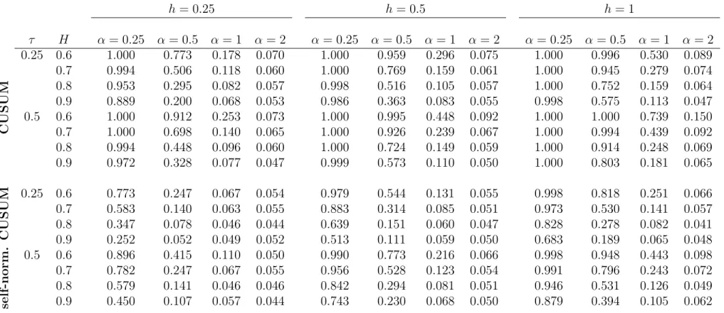
α= 0.05, the CUSUM test performs badly, while the self-normalized CUSUM works well. This is due to the fact that extremely large observations (due to small values of α) are misinterpreted as change-points. Furthermore, we can see from Table 3 that both tests detect change-points that are located in the middle of the sample with higher frequency than change-points that are located close to the boundary of the testing region. In the presence of a change in α, the number of test decisions in favor of the alternative increases as the height h of the level shift in the tail index increases. Moreover, it is notable that small values of α go along with a high number of rejections under the alternative as well. In particular, one can observe that the heavier the tails (i.e. the smaller α) the higher the rejection rate. This is very likely due to the aforementioned misinterpretation of the extremely large values as changes.
Comparing the rejection rates of the tests for different Hurst parameters, the follow-ing relation seems to hold: the bigger H, the smaller the number of rejections under the hypothesis and under the alternative. Under the alternative this may be due to the fact that the variance of the observations increases as the dependence, i.e. the values of the parameter H, increases (as suggested in Section 4.3). Therefore, it becomes harder to detect a level shift of a fixed height. The difference in rejection rates for differentH is less prominent in the self-normalized version of the test.
In general:
• The self-normalized test seems to be too conservative in the sense that the empirical size of the testing procedure is smaller than the significance level;
• The rejection rate of the classical CUSUM test is considerably higher than the nom-inal level of 5%.
• Under the alternative, the rejection rate of the classical CUSUM test is bigger than that of the self-normalized test for any choice of the parameters α and H.
As for the latter comment, in the context of change-point tests the so-called “better size but less power” phenomenon based on self-normalized statistics has been observed by [18], [19] and [4]. Moreover, it is consistent with observations made in [16] and [20]. It is important to note that the finite sample results are based on simulations which were executed under the assumption that the normalization dn,m, which depends on the parameters m, D and the
slowly varying functionL, and the coefficient Jm(Ψ) are known. For all practical purposes
this is not the case, so that both expressions have to be estimated. In contrast, the self-normalized test statistic can be computed from the given data while its limit depends on the parameters m and D only. For an adequate comparison of the testing procedures this has to be taken into consideration.
CUSUM self-normalized CUSUM n H α = 0.25 α = 0.5 α= 1 α = 2 α= 0.25 α= 0.5 α= 1 α= 2 50 0.6 0.961 0.567 0.168 0.065 0.024 0.031 0.032 0.041 0.7 0.902 0.428 0.126 0.060 0.012 0.019 0.030 0.045 0.8 0.849 0.343 0.115 0.060 0.005 0.010 0.024 0.042 0.9 0.847 0.340 0.099 0.058 0.005 0.004 0.021 0.039 100 0.6 0.971 0.544 0.156 0.066 0.022 0.031 0.037 0.045 0.7 0.880 0.366 0.107 0.060 0.019 0.024 0.035 0.047 0.8 0.754 0.248 0.097 0.060 0.007 0.015 0.030 0.043 0.9 0.701 0.223 0.083 0.057 0.005 0.009 0.028 0.042 200 0.6 0.969 0.510 0.148 0.068 0.024 0.029 0.038 0.047 0.7 0.819 0.296 0.096 0.060 0.016 0.026 0.041 0.052 0.8 0.605 0.191 0.074 0.056 0.008 0.020 0.037 0.042 0.9 0.492 0.146 0.075 0.053 0.007 0.021 0.044 0.047 300 0.6 0.964 0.486 0.146 0.067 0.0267 0.035 0.040 0.051 0.7 0.778 0.262 0.095 0.056 0.019 0.026 0.042 0.047 0.8 0.506 0.161 0.075 0.057 0.008 0.023 0.038 0.044 0.9 0.380 0.112 0.056 0.042 0.009 0.025 0.038 0.042 400 0.6 0.958 0.473 0.139 0.069 0.029 0.033 0.041 0.048 0.7 0.729 0.249 0.093 0.063 0.016 0.031 0.046 0.050 0.8 0.461 0.135 0.062 0.048 0.013 0.026 0.034 0.046 0.9 0.312 0.100 0.059 0.046 0.010 0.027 0.040 0.052 500 0.6 0.955 0.454 0.138 0.065 0.025 0.030 0.043 0.046 0.7 0.701 0.222 0.087 0.056 0.019 0.030 0.047 0.049 0.8 0.402 0.126 0.065 0.058 0.013 0.027 0.041 0.046 0.9 0.263 0.085 0.057 0.049 0.014 0.029 0.044 0.052 1000 0.6 0.937 0.424 0.125 0.065 0.032 0.037 0.041 0.047 0.7 0.595 0.179 0.073 0.056 0.022 0.032 0.046 0.046 0.8 0.295 0.100 0.063 0.054 0.016 0.037 0.045 0.045 0.9 0.171 0.079 0.052 0.047 0.020 0.043 0.049 0.048
Table 2: Rejection rates of the CUSUM change-point tests for stochastic volatility time series of lengthn which satisfy (14). The calculations are based on 5,000 simulation runs.
h= 0.25 h= 0.5 h= 1 τ H α = 0.25 α = 0.5 α= 1 α = 2 α= 0.25 α= 0.5 α= 1 α= 2 α = 0.25 α = 0.5 α= 1 α = 2 CUSUM 0.25 0.6 1.000 0.773 0.178 0.070 1.000 0.959 0.296 0.075 1.000 0.996 0.530 0.089 0.7 0.994 0.506 0.118 0.060 1.000 0.769 0.159 0.061 1.000 0.945 0.279 0.074 0.8 0.953 0.295 0.082 0.057 0.998 0.516 0.105 0.057 1.000 0.752 0.159 0.064 0.9 0.889 0.200 0.068 0.053 0.986 0.363 0.083 0.055 0.998 0.575 0.113 0.047 0.5 0.6 1.000 0.912 0.253 0.073 1.000 0.995 0.448 0.092 1.000 1.000 0.739 0.150 0.7 1.000 0.698 0.140 0.065 1.000 0.926 0.239 0.067 1.000 0.994 0.439 0.092 0.8 0.994 0.448 0.096 0.060 1.000 0.724 0.149 0.059 1.000 0.914 0.248 0.069 0.9 0.972 0.328 0.077 0.047 0.999 0.573 0.110 0.050 1.000 0.803 0.181 0.065 self-norm. CUSUM 0.25 0.6 0.773 0.247 0.067 0.054 0.979 0.544 0.131 0.055 0.998 0.818 0.251 0.066 0.7 0.583 0.140 0.063 0.055 0.883 0.314 0.085 0.051 0.973 0.530 0.141 0.057 0.8 0.347 0.078 0.046 0.044 0.639 0.151 0.060 0.047 0.828 0.278 0.082 0.041 0.9 0.252 0.052 0.049 0.052 0.513 0.111 0.059 0.050 0.683 0.189 0.065 0.048 0.5 0.6 0.896 0.415 0.110 0.050 0.990 0.773 0.216 0.066 0.998 0.948 0.443 0.098 0.7 0.782 0.247 0.067 0.055 0.956 0.528 0.123 0.054 0.991 0.796 0.243 0.072 0.8 0.579 0.141 0.046 0.046 0.842 0.294 0.081 0.051 0.946 0.531 0.126 0.049 0.9 0.450 0.107 0.057 0.044 0.743 0.230 0.068 0.050 0.879 0.394 0.105 0.062
Table 3: Rejection rates of the CUSUM change-point test for stochastic volatility time series of length n = 300 with Hurst parameter H and a change-point in the tail parameter α of height h after a proportion τ. The calculations are based on 5,000 simulation runs.
7
Appendix: Proof of Lemma
3.6
Prior to the proof of Lemma 3.6 we establish the following result:
Lemma 7.1. Let x < y and define
∆n(t;x, y) :=Mn(y, t)−Mn(x, t).
Then, E(Mn(x, t)) = 0, E(∆n(t;x, y)) = 0, and the following inequalities hold:
Var (Mn(x, t))≤ bntcFψ(X1)(x), Var (∆n(t;x, y))≤ bntc Fψ(X1)(y)−Fψ(X1)(x) . Proof. We have ∆n(t;x, y) = bntc X j=1 αj(x, y), where αj(x, y) := 1{x<ψ(Xj)≤y}−E 1{x<ψ(Xj)≤y}| Fj−1 . (15) Obviously, E bntc X j=1 αj(x, y) = 0. Furthermore, Var bntc X j=1 αj(x, y) = E bntc X j=1 αj(x, y) 2 = bntc X i=1 bntc X j=1 E (αi(x, y)αj(x, y)).
Note that for i < j we have E (αi(x, y)αj(x, y)) = E 1{x<ψ(Xi)≤y}−E 1{x<ψ(Xi)≤y}| Fi−1 1{x<ψ(Xj)≤y}−E 1{x<ψ(Xj)≤y}| Fj−1 = E 1{x<ψ(Xi)≤y}1{x<ψ(Xj)≤y} + E E 1{x<ψ(Xi)≤y}| Fi−1 E 1{x<ψ(Xj)≤y}| Fj−1 −E 1{x<ψ(Xi)≤y}E 1{x<ψ(Xj)≤y}| Fj−1 −E 1{x<ψ(Xj)≤y}E 1{x<ψ(Xi)≤y}| Fi−1 = E 1{x<ψ(Xi)≤y}1{x<ψ(Xj)≤y} + E E 1{x<ψ(Xj)≤y}E 1{x<ψ(Xi)≤y}| Fi−1 | Fj−1 −E E 1{x<ψ(Xi)≤y}1{x<ψ(Xj)≤y}| Fj−1 −E 1{x<ψ(Xj)≤y}E 1{x<ψ(Xi)≤y}| Fi−1 = E 1{x<ψ(Xi)≤y}1{x<ψ(Xj)≤y} + E 1{x<ψ(Xj)≤y}E 1{x<ψ(Xi)≤y}| Fi−1 −E 1{x<ψ(Xi)≤y}1{x<ψ(Xj)≤y} −E 1{x<ψ(Xj)≤y}E 1{x<ψ(Xi)≤y}| Fi−1 = 0.
Due to stationarity we have E α2i(x, y) = Eh 1{x<ψ(Xi)≤y} −E 1{x<ψ(Xi)≤y}| Fi−1 2i = E1{x<ψ(Xi)≤y} −E1{x<ψ(Xi)≤y}E 1{x<ψ(Xi)≤y}| Fi−1 ≤Fψ(X1)(y)−Fψ(X1)(x). It follows that Var bntc X j=1 αj(x, y) = bntc X j=1 E α2j(x, y) ≤ bntc Fψ(X1)(y)−Fψ(X1)(x) .
Proof of Lemma 3.6. In order to prove Lemma3.6we have to verify tightness inD([−∞,∞]×
[0,1]). For this we quote Theorem 3 in [14], adapted toD([−∞,∞]×[0,1]), i.e. we assume that the following theorem holds:
Theorem 7.2. Let Xn(x, t)be a sequence of random elements of D([−∞,∞]×[0,1]) and let Tk
n denote a natural k-stopping time for Xn(x, t). If Xn(x, t) is tight on the line for each (x, t) ∈ [−∞,∞]×[0,1] and if for all δn & 0, all C > 0 and all uniformly bounded
Tk n sup 0≤t≤1 Xn(Tnk+δn, t)−Xn(Tnk, t) P −→0, as n→ ∞, (16) sup −C≤x≤C Xn(x, Tnk+δn)−Xn(x, Tnk) P −→0, as n→ ∞, (17) then Xn is tight in D([−∞,∞]×[0,1]).
In the following we will show that the conditions of the theorem hold for Xn(x, t) :=
n−1/2M
n(x, t). Then, Lemma 3.6 immediately follows from an application of Theorem
7.2. Indeed, due to Lemma 3.5 n−1/2M
n(x, t) is tight for each (x, t) ∈ (−∞,∞)×[0,1].
Therefore, it remains to show (16) and (17). LetTk
n denote a natural, uniformly boundedk-stopping time forXn(x, t). Thus,|Tnk| ≤
M for some M >0 and for all n. Define τn :=bnTnkc.
Note that 1 √ nMn(x, T k n +δn)− 1 √ nMn(x, T k n) = 1 √ n τn+bnδnc X j=τn+1 ξj(x, ω) ,
where ξj(x, ω) := (ξj(x)) (ω). For C > 0 we have P ω : sup −C≤x≤C 1 √ n τn(ω)+bnδnc X j=τn(ω)+1 ξj(x, ω) > ε = M X m=0 P ω: sup −C≤x≤C 1 √ n τn(ω)+bnδnc X j=τn(ω)+1 ξj(x, ω) > ε ∩ {ω|τn(ω) =m} ≤ M X m=0 P ω: sup −C≤x≤C 1 √ n m+bnδnc X j=m+1 ξj(x, ω) > ε = M X m=0 P ω: sup −C≤x≤C 1 √ n bnδnc X j=1 ξj(x, ω) > ε = (M+ 1)P sup −C≤x≤C 1 √ nMn(x, δn) > ε .
Therefore, to show (17), it suffices to prove that sup −C≤x≤C ˜ Mn(x) P −→0, asn → ∞, (18) with ˜ Mn(x) := 1 √ nMn(x, δn).
Due to Lemma 7.1, E( ˜Mn(x)) = 0 and Var( ˜Mn(x)) ≤ δnFψ(X1)(x) −→ 0, hence ˜Mn(x)
converges to 0 in probability. This implies fidi-convergence of ˜Mn as a process with values
inD[−C, C]. In order to show tightness of ˜Mn, we adopt the argument that proves Theorem
15.6 in [5]. For any function v in D[−C, C] define the modulus ωv00(δ) by
ω00v(δ) = sup min{|v(t)−v(t1)|,|v(t2)−v(t)|}, where the supremum extends over t1, t, and t2 satisfying
t1 ≤t≤t2, t2 −t1 ≤δ.
Under the assumption of fidi-convergence it suffices to show that for each positive ε and
η, there exists a δ, 0< δ <1, and an integer n0 such that
Pn ω00M˜ n(δ)≥ε ≤η, n≥n0, (see Theorem 15.4 in [5]).
Define Mm00 := max 0≤i≤j≤k≤mmin{|Sj −Si|,|Sk−Sj|}, where Si = ˜Mn(τ + mi δ). By Theorem 12.5 in [5] P Mm00 ≥λ≤ K λ2(u1+. . .+um) 2 (19)
holds for all positive λ and some constant K, if
P({|Sj −Si| ≥λ,|Sk−Sj| ≥λ})≤ 1 λ2 X i<l≤k ul ! , 0≤i≤j ≤k≤m. Forx1 ≤x≤x2 we have ˜ Mn(x1)−M˜n(x) = 1 √ n bnδnc X j=1 αj(x1, x) , ˜ Mn(x)−M˜n(x2) = 1 √ n bnδnc X j=1 αj(x, x2)
with αj defined by (15). Because of the Cauchy - Schwarz inequality for expected values
and Lemma 7.1 it follows that E 1 √ n bnδnc X j=1 αj(x1, x) 1 √ n bnδnc X j=1 αj(x, x2) ≤ v u u u t 1 nE bnδnc X j=1 αj(x1, x) 2 1 nE bnδnc X j=1 αj(x, x2) 2 ≤δn Fψ(X1)(x2)−Fψ(X1)(x1) . (20) The Markov inequality yields
P (|Sj−Si| ≥λ,|Sk−Sj| ≥λ)≤P |Sj−Si| |Sk−Sj| ≥λ2
≤ 1
λ2 E|Sj −Si| |Sk−Sj|. Therefore, it follows by (20) that
P(|Sj −Si| ≥λ,|Sk−Sj| ≥λ)≤ 1 λ2 k X l=i+1 ul
with ul :=δn Fψ(X1) τ + l mδ −Fψ(X1) τ+ l−1 m δ . As a result, we have P Mm00 ≥ε≤ K ε2 m X l=1 ul = K ε2δn Fψ(X1)(τ +δ)−Fψ(X1)(τ) . Define ω00( ˜Mn,[τ, τ +δ]) := sup min n |M˜n(t)−M˜n(t1)|,|M˜n(t2)−M˜n(t)| o ,
where the supremum extends over t1, t, t2 satisfying τ ≤ t1 ≤ t ≤ t2 ≤ τ +δ. Letting
m−→ ∞ in (19) yields P ω00( ˜Mn,[τ, τ +δ])≥ε ≤ K ε2δn Fψ(X1)(τ+δ)−Fψ(X1)(τ) (21) due to right-continuity of ˜Mn. Suppose that δ= Cu for some integer u and assume that
ω00( ˜Mn,[−C+ 2iδ,−C+ (2i+ 2)δ])≤ε, 0≤i≤u−1, (22)
ω00( ˜Mn,[−C+ (2i+ 1)δ,−C+ (2i+ 3)δ])≤ε, 0≤i≤u−2. (23)
If t1 ≤ t ≤ t2 and t2 − t1 ≤ δ, then t1 and t2 both lie in one of the 2u−1 intervals [−C+ 2iδ,−C+ (2i+ 2)δ], 0≤i≤u−1, [−C+ (2i+ 1)δ,−C+ (2i+ 3)δ], 0≤i≤u−2, so that min n ˜ Mn(t)−M˜n(t1) , ˜ Mn(t2)−M˜n(t) o ≤ε.
Thus, (22) and (23) together imply ωM00˜
n(δ)≤ε. It now follows by (21) that
PωM00˜ n(δ)≥ε ≤ K ε2δn(Σ 0 + Σ00),
where each of Σ0 and Σ00 is a sum of the form
r X
k=1
Fψ(X1)(tk)−Fψ(X1)(tk−1)
with −C ≤t1 ≤. . .≤tr ≤C and tk−tk−1 ≤2δ. Hence, we may conclude that
P ωM00˜ n(δ)≥ε ≤ 2K ε2 δn Fψ(X1)(1)−Fψ(X1)(0) .
Thus, it remains to show (16). Note that sup 0≤t≤1 Xn(Tnk+δn, t)−Xn(Tnk, t) = sup 0≤t≤1 |Mn∗(t)| with Mn∗(t) := √1 n bntc X j=1 1{0≤ψ(Xj)≤δn}−E 1{0≤ψ(Xj)≤δn}| Fj−1 .
Lemma7.1yields E(Mn∗(t)) = 0 and Var(Mn∗(t))≤t Fψ(X1)(δn)−Fψ(X1)(0)
. Thus,Mn∗(t) converges to 0 in probability to continuity of Fψ(X1). This implies fidi-convergence of M
∗
n
as a process with values in D[0,1]. Again, we make use of Theorem 15.4 in [5], i.e. we verify that for each positive ε and η, there exists a δ, 0 < δ < 1, and an integer n0 such that Pn ω00M∗ n(δ)≥ε ≤η, n≥n0. Define Mm00 := max 0≤i≤j≤k≤mmin{|Sj −Si|,|Sk−Sj|}, where Si =Mn∗(τ + i mδ). We have |Mn∗(t1)−Mn∗(t)|= 1 √ n bntc X j=bnt1c+1 αj(0, δn) , |Mn∗(t)−Mn∗(t2)|= 1 √ n bnt2c X j=bntc+1 αj(0, δn) ,
where αj as defined before. The Cauchy-Schwarz inequality yields
E|Mn∗(t1)−Mn∗(t)| |M ∗ n(t)−M ∗ n(t2)| = E 1 √ n bntc X j=bnt1c+1 αj(x1, x) 1 √ n bnt2c X j=bntc+1 αj(x, x2) ≤p(t−t1)(t2−t) Fψ(X1)(δn)−Fψ(X1)(0) ≤(t2−t1) Fψ(X1)(δn)−Fψ(X1)(0) .
By the same argument as in the proof of (17) it follows that
P (|Sj−Si| ≥λ,|Sk−Sj| ≥λ)≤ 1 λ2 k X l=i+1 ul,
with ul := Fψ(X1)(δn)−Fψ(X1)(0)
1 mδ.
Therefore, Theorem 12.5 in [5] yields
P Mm00 ≥ε≤ K
ε2δ Fψ(X1)(δn)−Fψ(X1)(0)
.
Taking the right-continuity of Mn∗ into consideration, we may, as before, conclude that
P ωM00 ∗ n(δ)≥ε ≤ K ε2δ Fψ(X1)(δn)−Fψ(X1)(0) .
Due to continuity ofFψ(X1) the right-hand side of the above inequality vanishes as ntends
to∞. This concludes the proof of (16) as well as the proof of Lemma 3.6.
References
[1] Donald W. K. Andrews. Tests for parameter instability and structural change with unknown change point. Econometrica, 61:821–856, 1993.
[2] Jan Beran, Yuanhua Feng, Sucharita Ghosh, and Rafal Kulik.Long memory processes. Springer, 2013.
[3] I. Berkes, L. Horv´ath, P. Kokoszka, and Q.-M. Shao. On discriminating between long-range dependence and changes in mean. Annals of Statistics, 34(3):1140–1165, 2006.
[4] Annika Betken. Testing for change-points in long-range dependent time series by means of a self-normalized wilcoxon test. Journal of Time Series Analysis, 37(6):721– 864, 2016.
[5] Patrick Billingsley. Convergence of Probability Measures. John Wiley & Sons, Inc., 1968.
[6] Patrick Billingsley. Convergence of Probability Measures. John Wiley & Sons, Inc., 1999.
[7] F. Jay Breidt, Nuno Crato, and Pedro de Lima. The detection and estimation of long memory in stochastic volatility. Journal of Econometrics, 83(1-2):325–348, 1998. [8] M. Cs¨org¨o and L. Horvath. Limit Theorems in Change-Point Analysis. Wiley, New
York., 1997.
[9] Herold Dehling, Aeneas Rooch, and Murad S. Taqqu. Non-parametric change-point tests for long-range dependent data. Scandinavian Journal of Statistics, 40(1):153— 173, 2013.
[10] Herold Dehling and Murad Taqqu. The empirical process of some long-range de-pendent sequences with an application to U-statistics. The Annals of Statistics, 17(4):1767—1783, 1989.
[11] Aryeh Dvoretzky. Asymptotic normality for sums of dependent random variables. Pro-ceedings of the Sixth Berkeley Symposium on Mathematical Statistics and Probability, 2:513–535, 1972.
[12] Liudas Giraitis, Remigijus Leipus, and Donatas Surgailis. The change-point problem for dependent observations. Journal of Statistical Planning and Inference, 53:297 – 310, 1996.
[13] L. Horv´ath and P. Kokoszka. The effect of long-range dependence on change-point estimators. Journal of Statistical Planning and Inference, 64(1):57–81, 1997.
[14] Gail Ivanoff. Stopping times and tightness for multiparameter martingales. Statistics & probability letters, 28(2):111–114, 1996.
[15] Rafa l Kulik and Philippe Soulier. The tail empirical process for long memory stochastic volatility sequences. Stochastic Processes and their Applications, 121(1):109 – 134, 2011.
[16] Ignacio N. Lobato. Testing that a dependent process is uncorrelated. Journal of the American Statistical Association, 96:1066–1076, 2001.
[17] Sidney I. Resnick. Heavy-tail phenomena. Springer Series in Operations Research and Financial Engineering. Springer, New York, 2007. Probabilistic and statistical modeling.
[18] Xiaofeng Shao. A simple test of changes in mean in the possible presence of long-range dependence. Journal of Time Series Analysis, 32:598 – 606, 2011.
[19] Xiaofeng Shao and Xianyang Zhang. Testing for change points in time series. Journal of The American Statistical Association, 105:1228 – 1240, 2010.
[20] Yixiao Sun, Peter C. B. Phillips, and Sainan Jin. Optimal bandwidth selection in heteroskedasticity autocorrelation robust testing. Econometrica, 76:175–194, 2008. [21] Murad S. Taqqu. Convergence of integrated processes of arbitrary Hermite rank.
Zeitschrift f¨ur Wahrscheinlichkeitstheorie und Verwandte Gebiete, 50(1):53–83, 1979. [22] Johannes Tewes. Change-point tests under local alternatives for long-range dependent