Efficient Measurement of Data Flow
Enabling Communication-Aware Parallelisation
Peter Bertels
[email protected]
Wim Heirman
[email protected]
Dirk Stroobandt
[email protected]
Department of Electronics and Information Systems Ghent University, Sint-Pietersnieuwstraat 41, 9000 Gent, Belgium
ABSTRACT
As multicore chips scale to higher processor counts, commu-nication between cores becomes more and more important. Indeed, when a single application is split up among mul-tiple cores, which are connected through a relatively slow network, the amount of communication that is required will have an essential effect on performance. Therefore, if the application can be partitioned in such a way that commu-nication between threads is minimised, or that placement on non-uniform networks can be performed with regards to communication, a significant performance boost can be ob-tained. But to do this effectively, communication streams inside the application must be known. In this paper, we in-troduce a profiling tool for Java that can measure data flows between methods. It constructs a communication graph, which combines a traditional call graph with data flow in-formation.
The overhead of profiling is brought down by a factor of 15 through the use of reservoir sampling. We prove that this can be done with a limited decrease in accuracy.
This way, we can quickly estimate communication flows, which forms the critical information that allows an efficient communication-aware parallelisation to be made.
Categories and Subject Descriptors
D.4.8 [Software Engineering]: Performance—measurements, simulation, stochastic analysis
General Terms
Data-flow; profiling
1.
INTRODUCTION
As multicore chips scale to higher processor counts, com-munication between cores becomes more and more impor-tant. On a typical multicore architecture one can distin-guish several levels of communication, each with different
performance characteristics: threads executed on the same core communicate by means of shared memory in an on-chip cache or in in an off-chip memory only reachable through the network; threads executed on different cores can only use the relatively slow network connection. This essential difference between internal and external communication as well as the amount of inter-thread communication have a crucial impact on the final performance when a single ap-plication is split up among multiple cores. Therefore, if the application can be partitioned in such a way that commu-nication between threads is minimised, or that placement on non-uniform networks can be performed with regards to communication, a significant performance boost can be ob-tained. But to do this effectively, communication streams inside the application must be known.
In this paper, we introduce a profiling tool for Java that can measure data flows between methods. It constructs a com-munication graph, which combines a traditional call graph with data flow information. This combined view gives the programmer the basic information needed for the paralleli-sation process in which several methods in the application will be combined into threads: computational requirements, dependencies and data flow measurements.
Our main contribution is the communication graph: an ex-tension of a call graph with information on the inherent com-munication flow in the application, defined in Section 2. The weights of each node in our communication graph indicate the required computational power for this method; this in-formation is used by the programmer to constrain the num-ber of nodes put together in a single thread. The edges of the call graph represent dependencies which will determine the possible scheduling of the application on multiple cores. New in our approach is the effectively measured amount of communication between methods. This additional informa-tion enables a truly communicainforma-tion-aware parallelisainforma-tion.
The amount of communication within a program is indepen-dent of the implementation. Indeed, parallelisation does not change the inherent communication, it only influences the ratio of internal and external communication, which in turn, influences performance. Because of this implementation in-dependence, we can measure the inherent communication during the execution of the program on a simple, single core processor.
is well-suited for program analysis and for profiling. The multi-threaded nature of the language offers the opportunity to model concurrent behaviour. This gives us the opportu-nity to not only profile the original single-threaded applica-tion, but to also profile the application after (or even during) the parallelisation process. This way the programmer can have direct feedback on the reduction in communication cost he has realised by appropriately parallising the application. Section 3 explains how Java programs are profiled in order to build the communication graph. It should be mentioned that although the work in this paper is implemented com-pletely in Java, the underlying principles are portable to C as well. Changing the Java profiler to a native x86 profiling framework will do.
Profiling the Java program causes a huge increase in ex-ecution time due to the extensive bookkeeping: we have to keep track of every memory read or write. To reduce this overhead we implement reservoir sampling [5]. This sampling method enables communication estimation with a pre-specified accuracy and acceptable overhead. Section 4 introduces reservoir sampling and discusses its accuracy and practical limitations.
Our approach is evaluated on the SPECjvm98 benchmark suite [4]. Section 5 shows the most important properties of the resulting communication graphs. This section also shows how reservoir sampling could reduce the profiling overhead by a factor of 15 on average and we give experimental results for the obtained accuracy.
A comparison with related work is made in Section 6 and in Section 7, concluding remarks follow.
2.
COMMUNICATION GRAPH
Within programs, data flows from producers to consumers. That is, some methods in a program calculate values and store them in memory, i.e. these methods produce the data. Other methods need to use this data and read it from mem-ory. These methods are consumers. Each producer-consumer pair leads to communication in the final implementation. Therefore we will call this inherent communication. This communication will be measured and captured in a commu-nication graph.
We assume that this inherent communication, available in the original program, will remain in the final implementa-tion after parallelisaimplementa-tion. Methods in the executable speci-fication will be grouped into threads and mapped onto (dif-ferent) cores on the multicore architecture, but as long as the underlying algorithm remains, the communication be-tween methods will not change. Therefore our communica-tion graph will be completely implementacommunica-tion independent. When the programmer changes the program, e.g. while per-forming specific optimisations in order to further reduce the communication, the initial assumption does not hold any-more and the communication graph has to be rebuilt.
2.1
Example
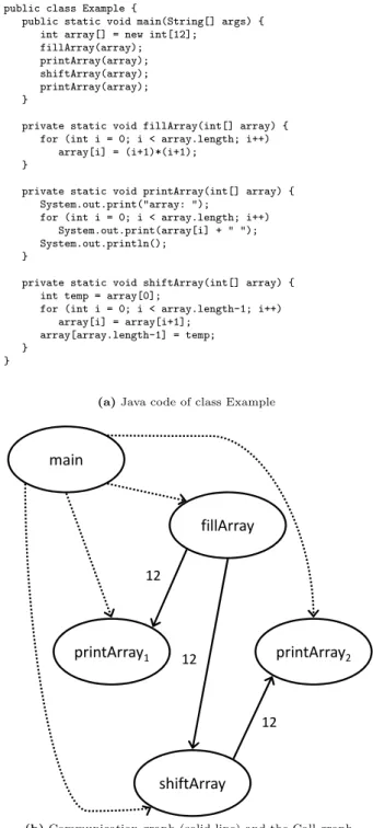
As an introduction, a simple example of a Java program and its communication graph is given in Figure 1. A rigorous definition follows in the next subsection.
public class Example {
public static void main(String[] args) { int array[] = new int[12];
fillArray(array); printArray(array); shiftArray(array); printArray(array); }
private static void fillArray(int[] array) { for (int i = 0; i < array.length; i++)
array[i] = (i+1)*(i+1); }
private static void printArray(int[] array) { System.out.print("array: ");
for (int i = 0; i < array.length; i++) System.out.print(array[i] + " "); System.out.println();
}
private static void shiftArray(int[] array) { int temp = array[0];
for (int i = 0; i < array.length-1; i++) array[i] = array[i+1];
array[array.length-1] = temp; }
}
(a)Java code of class Example
main
fillArray
12printArray
1printArray
2shiftArray
12 12(b)Communication graph (solid line) and the Call graph (dotted line)
array: 1 4 9 16 25 36 49 64 81 100 121 144 array: 4 9 16 25 36 49 64 81 100 121 144 1
(c)Console output
Themain method of theExample class creates an array of 12 integers, which is filled with 1,4,9,16, . . .byfillArray. When the printArray method is called for the first time to print these numbers to the console, method printAr-ray consumes the values which were produced by method
fillArray. This can be seen in the communication graph as a solid edge with label 12 from node fillArray to node
printArray1.
After filling and printing the array,maincalls the shiftAr-raymethod to shift the values in the array. The shifted array is then printed by a second call of printArray. This makes methodshiftArraya consumer of the values produced by
fillArray and a producer for the new values used by the
printArray method. The communication graph therefore
contains two more solid edges: an edge from fillArray to
shiftArray and another one fromshiftArray toprintArray2.
It should be noticed that the two calls to methodprintArray
are represented in the communication graph by two different nodes printArray1 and printArray2. As can be seen from
Figure 1 (b), our communication graph also contains a call graph. Edges of the call graph are represented as dotted lines.
2.2
Communication Graph
The communication graphGis a directed graph, defined by a set of nodesV and two sets of directed edges: E1 andE2.
The vertices inV representcommunicating partners. These communicating partners are producers and/or consumers of data. They form the finest granularity for our profiling. In the previous example, each method invocation introduced a new communicating partner in the graphG. Sometimes a coarser view of the execution is more appropriate. Sev-eral alternatives for grouping producers and consumers into communicating partners will be discussed in the next sub-section.
The edges in setE1are weighted edges. These edges
repre-sent the amount of data flowing between two communicating partners, measured in bytes of the complete the runtime of the application. The non-weighted edges inE2represent the
call graph of the program. Each edge points from a caller to a callee.
In this paper we present a methodology to build the com-munication graph during the execution of a program. It should be mentioned that this graph is a representation of the communication during this specific execution. For non-deterministic programs the result may vary from execution to execution.
This definition of a communication graph, brings us to a definition of producer-consumer pair. A pair of communi-cating partners (p, c) is a producer-consumer pair when: the producer p has written some data d in memory and later on the consumerc had read this same datad without any other communicating partner has written to d in between the production and the consumption.
This definition is useful for single-threaded applications as well as for multi-threaded applications in which the producer
and the consumer might be in different threads.
2.3
Practical Considerations
The communication graph is built by analysing the execu-tion of a Java program. In Java the producers and con-sumers of data are individual bytecode instructions, which are interpreted by the Java Virtual Machine. This enables us to measure local data flow between these bytecodes. This local information is neglected nevertheless, because global data flow between methods is more important for paralleli-sation than local data flow.
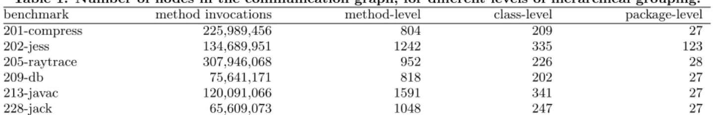
In order to capture global data flow in the communication graph, we decided to consider methods as the finest granu-larity for the profiling. This means that one communicat-ing partner surveys information about the data production and consumption of one invocation of a certain method. For small programs, as the above example, this may be a good choice, but for larger programs this granularity is too fine and this results in an unmanageable number of nodes. The number of method invocations in the programs of the SPECjvm98 benchmark suite can be found in Table 1.
To keep the communication graph manageable, we have to raise the abstraction level by reducing the number of nodes. This is done by grouping several nodes into bigger nodes. For this grouping we implemented various alternatives that are based on one of the following important properties of the Java language.
Hierarchy Java programs inherently have a hierarchical structure. Methods are declared within classes, which are part of packages. These abstraction levels can be used by our profiler too. As explained earlier the finest level is that where individual method invocations have their own node in the communication graph. At the method level, all invocations of the same method are grouped in one communicating partner. At class level even all methods declared in the same class are grouped. The abstraction can be raised further by grouping all methods declared in the same package. The resulting number of nodes in the entire communi-cation graph for these three abstraction levels (method-level, class-level and package-level) is shown in Table 1.
Call Tree Apart from the statical grouping using the Java class hierarchy, our profiler can also perform a dynamic grouping of nodes based on the call graph. Instead of creating a new node in the communication graph for each invocation of every method, the call tree mode of our profiler will group all method invocation with the same call stack in a single node.
Concurrency Java can express concurrent behaviour by implementing parallel threads. Our profiler is initially meant for profiling single-threaded applications, but it can also measure communication between different threads. Each thread is then considered as a communi-cating partner and has thus its own node in the com-munication graph. This gives us the opportunity to profile the application after (or even during) the paral-lelisation process. This way the programmer can have direct feedback on the reduction in communication
object field0 field1 field2 field3 global map shadow1 producer0 producer1 producer2 producer3 CommID1 CommID2 array a[0] shadow2 producer0 a[0] a[1] ... a[N] producer0 producer1 ... producerN CommID3
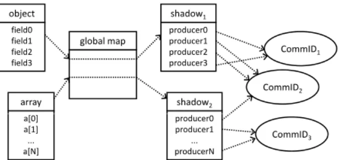
Figure 2: Objects and the corresponding shadow objects.
cost realised by performing communication-related op-timisations. Since the SPECjvm98 benchmark is single-threaded, this way of grouping is not included in Ta-ble 1.
It is also possible to extend these possible granularity levels to loop-level profiling where individual loops can be treated as communicating partners. Although it is a logical exten-sions, this loop-level profiling is not yet implemented.
3.
PROFILING THE JAVA PROGRAM
3.1
Basic Idea
We want to build the graph defined in the previous section while running a Java program. We do this by instrumenting the Java code in order to capture every single read or write operation and to perform special actions to build the graph.
The basic idea of our approach is that every data field for each object in the Java heap memory is annotated with a reference to the communicating partner which has written the current value of this field. Whenever a read operation occurs in the program (consumption of data) we need to add an edge in the communication graph. This edge connects the communicating partners of the producer and the consumer of the data. The consumer apparently is the method which performed the read operation; the producers can be quickly identified by means of the last-writer information which was annotated when the field was written.
Note that this approach requires us to instrument every write operation which causes a huge overhead in execution time. The annotations of the last writer to each data field in memory causes an overhead in memory consumption.
3.2
Data Structures Used for Profiling
Two important data structures are introduced to enable this profiling. First, there isCommIDobjects representing commu-nicating partners. Secondly, for each object or array in the Java Virtual Machine (JVM), a Shadow object is created. These shadow objects contain information about the pro-ducers of the data in every field in the object or every index in the array.
Figure 2 shows a concrete example with an object and an array. As can be seen in this figure, the profiler maintains a global map, which maps object or array references to their
corresponding shadow object. Every field in the shadow object links to a communicating partner represented by its
CommIDobject.
It should be mentioned that this CommID objects are also used as nodes in the final communication graph.
3.3
Instrumentation
In order to perform the profiling, special instrumentation code has to be inserted in the original Java program. We are instrumenting the Java code at runtime, which enables us to instrument the Java program as well as all standard libraries used by this program. This is an important advan-tage because methods in the standard libraries are respon-sible for a significant fraction of the total communication in the system.
Moreover our instrumentation is targeted directly on the Java bytecode, the lowest abstraction level within the JVM. Therefore not a single byte of communication in the pro-gram, is hidden for our profiler. Notwithstanding the low abstraction level, the Java bytecode still contains the high level structure of the program as well as type information for the data that is used.
4.
RESERVOIR SAMPLING
Every producer-consumer pair in the program has to be analysed by our profiler. Due to the large number of read and write operations this causes a huge overhead in execu-tion time as well as in memory consumpexecu-tion. By reducing the amount of producer-consumer pairs to be analysed, the overhead can be reduced considerably.
A read operation in the program directly leads to a producer-consumer pair. The aim of the sampling method is thus to select a limited number of read operations to be taken into account for building the communication graph with an ac-ceptable accuracy. In this paper we propose to apply reser-voir sampling [5] to achieve this aim. Section 4.1 explains the general principle of reservoir sampling as well as some important properties of this technique.
Although sampling reduces the overhead, it results in errors in the communication graph. Through the fact that reser-voir sampling selects a uniform random sample of producer-consumer pairs in the program, we can guarantee the error to be within a specified confidence interval. A statistical discussion is given in Section 4.2.
4.1
The Principle of Reservoir Sampling
The aim of reservoir sampling is to reduce the amount of measurement data by randomly selecting a limited number of samples from the original set, without the need to know the size of the data set beforehand.
Reservoir sampling works as follows: initially, the first n
samples of the original set are placed in the reservoir. Start-ing from sample n+ 1 every sample is evaluated one at a time. A random decision is made whether or not to add this samplemto the reservoir. If so, a random sample 06a < n
is chosen from the reservoir and this sample a is replaced by sample m. This algorithm leads to a set of exactly n
Table 1: Number of nodes in the communication graph, for different levels of hierarchical grouping.
benchmark method invocations method-level class-level package-level
201-compress 225,989,456 804 209 27 202-jess 134,689,951 1242 335 123 205-raytrace 307,946,068 952 226 28 209-db 75,641,171 818 202 27 213-javac 120,091,066 1591 341 27 228-jack 65,609,073 1048 247 27
samples, independent of the size of the data set. It can be proven [5] that thesensamples form a uniform and random sample set.
In the beginning most records are selected to be stored in the reservoir, but as the algorithm continues, more and more records are skipped, i.e. the probability of a record to be put in the reservoir decreases during the run of the algorithm. We implemented an extension to the basic principle, algo-rithm L described in [2]. Instead of randomly deciding, for each record individually, whether it should be added to the reservoir, algorithm L directly makes a random decision of the number of records to be skipped each time a record is selected. This enables speeding up the reservoir sampling process without sacrificing the statistical properties. Indeed, Li [2] proves that the probability distribution of algorithm L is the same as the original algorithm.
4.2
Statistical Discussion
The most important advantage of reservoir sampling over other techniques, is the fact that it provides a uniform ran-dom sample set. This allows following analysis.
The aim of our profiling is to estimate the amount of data flowing over every edge in the communication graph. In the non sampled version we can obtain absolute values, for the sampled version we want to estimate the relative importance of each edge, the fraction of the total communication which is going over this edge.
Let Fe be the fraction of communication going over edge
e. This fraction can be calculated asf /N, where f is the total number of producer-consumer relations on this edgee
andN is the total number of producer-consumer relations in the complete communication graphG. The estimation
ˆ
FeofFe will be calculated asc/n, wherecis the number of producer-consumer pairs on edge e in the sample set with sizen.
According to [6] the large sample confidence interval for ˆFe
is given by ˆ Fe±zα/2 s √ n, (1)
wheresis the sample standard deviation. The sample vari-ances2can be computed as
s2= n Pn i=1x 2 i− Pn i=1xi 2 n(n−1) . (2)
In our case xi are either 1 (producer-consumer relation is on edgee) or 0 (producer-consumer relation is on another
edge). Therefore our sample variances2 can be written as
s2= nc−c
2
n(n−1), (3)
which makes that
s √ n = r (c/n)(1−c/n) n−1 = s ˆ Fe(1−Feˆ) n−1 . (4)
The expected relative errorrfor a givenα% confidence in-terval can be defined as
r=zα/2
s
ˆ
Fe(1−Feˆ)
n−1 /Fe.ˆ (5)
This expression can be rearranged in order to calculate the number of samples n necessary to obtain a given relative errorr, for an expected accuracyFe. This results in:
n>zα/2
1−Fe
r2Fe . (6)
The following particular example illustrates this approach. In order to obtain, with 95% probability (zα/2 = 1.96), an
estimation that is accurate to within 5%, of the bandwidth for edges, representing a fraction of at least 0.1% of the total communication graph (Fe >0.1%), we need at least 1,535,048 samples.
It should be mentioned that this statistical discussion only covers important bandwidths in the system. Communica-tion over edges representing smaller bandwidths (Fe<0.1%) can only be estimated accurately when all producer-consumer pairs are taken into account. A sampled approach, reservoir sampling or any other sampling technique, cannot guaran-tee any accuracy at all for such small bandwidths. However, small bandwidths barely influence the communication cost so this approximation should have no effect on the overall system performance.
5.
RESULTS
We evaluated our approach with the SPECjvm98 benchmark suite. The six programs were run on an Opteron 242 with clock frequency 1.6 GHz and 4 GiB RAM memory.
In our first experiment we measured the communication graph for the SPECjvm98 programs. We did a full profiling with the finest granularity, i.e. every method invocation was measured separately. Table 1 illustrates the extensiveness of the resulting communication graphs.
1000 1200 1400 1600 1800 2000 sl o w d o w n f a ct o r samp1k samp10k samp100k samp1m 0 200 400 600 800 1000 0 5 10 15 20 25 sl o w d o w n f a ct o r
original execution time (s)
Figure 3: Relative slowdown factor in function of the original execution time
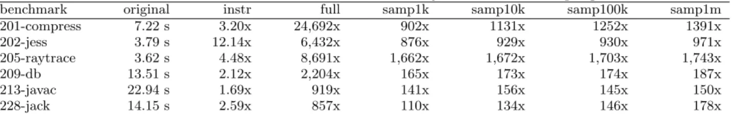
In a second experiment we used reservoir sampling for profil-ing the same communication graphs. We found that reser-voir sampling can drastically reduce the overhead in exe-cution time for the profiling: a reduction by factor of 15 on average. These results are shown in Table 2. Column
original in this table gives the original execution time for running the benchmarks. Columninstr shows the overhead introduced by the instrumentation framework, this is a rel-ative factor. For these instrumentation overhead results a Java agent was written that intercepts all classes, interpretes the bytecodes with ASM, and reassembles the classes with-out modification. The relative overhead in execution time for a full, non-sampled profiling is presented in the fourth columnfull. The next columns show the relative overhead for the reservoir sampled approach with different reservoir sizes: from 1000 samples in columnsamp1k up to 1 million samples in columnsamp1m.
Table 3 presents absolute figures for the total average mem-ory use of the original execution of the benchmarks. Rel-ative figures are included for the overhead introduced by the instrumentation, for the full profiling as well as for the reservoir sampled approach.
The sampled approach reduces the overhead drastically. The sampling overhead decreases as the program runs longer. Because each of the six benchmark programs has a different execution time, we can plot the slowdown factor in func-tion of the original execufunc-tion time in Figure 3. We did this for four different sizes of the sampling reservoir. The out-lier in this graph is the program 202-jess which has rela-tively more memory read/write operations than the other programs in the benchmark suite. Because of this, 202-jess benefits more from the ever increasing number of samples that can be skipped in the reservoir sampling algorithm.
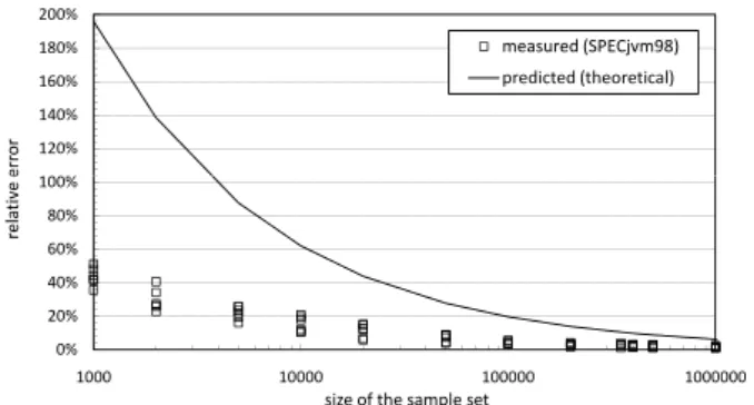
To conclude this section, we evaluated the accuracy of this sampling method. Figure 4 compares the measured rela-tive error (MRE) on the communication graph with the pre-dicted relative error obtained in Section 4.2. This measured relative error is defined as
MRE = v u u t 1 M M X i=1 ˆ Fe,i−Fe,iˆ Fe,i 2
,(7)where Fe,i is the actual relative weight of edge i in
100% 120% 140% 160% 180% 200% re la ti v e e rr o r measured (SPECjvm98) predicted (theoretical) 0% 20% 40% 60% 80% 100% 1000 10000 100000 1000000 re la ti v e e rr o r
size of the sample set
Figure 4: Relative error in function of the size of the sample set.
the communication graphG, ˆFe,i is the estimated relative weight of edge i in the sampled graph. Only theM most important edges wheree,i>0.1% are taken into account in
this equation.
This comparison proves that the predicted accuracy is also achieved in practice. The solid curve in this figure presents the predicted error for a 95% confidence interval, for band-widths representing more than 0.1% of the total bandwidth in the full communication graph. This explains the notice-able gap between the measured errors and the predicted er-ror. Most edges in the communication graph represent more than 0.1% of the total bandwidth and therefore they can be estimated more accurately.
6.
RELATED WORK
This section presents other graphs representing data flow in a program. Some of these represent a static view of the pro-gram, others depict information on the dynamic behaviour of the program. This distinction is crucial as it determines the possible use of the graphs.
Static Data Flow Graphs (SDFG), for instance, allow com-pilers to statically analyse data dependencies between state-ments in a code fragment. This static analysis enables the compiler to make sound decisions on, among other, the reg-ister allocation and optimisation. For concurrent Java code the Multithreaded Dependence Graph (MDG), an exten-sion of the SDFG, is introduced by Zhao who used the MDG for program slicing [7]. Although SDFGs could pos-sibly be used for parallelisation, they lack dynamic infor-mation on communication streams in the application, in contrast to our communication graph which truly facilitates communication-aware parallelisation.
Nethercote and Mycroft presented Redux [3], a profiling tool that builds a dynamic data flow graph while running a pro-gram. This is similar to our communication graph, but it dif-fers in the abstraction level: Redux measures data flow on a low abstraction level, namely between individual x86 assem-bly instructions. For communication estimation in the con-text of parallelisation, our intention, measuring at a higher abstraction level is more useful: the use of Java enables us to capture high level type information for the edges in the communication graph. This is impossible for Redux as this
Table 2: Overhead in execution time for SPECjvm98 benchmark programs
benchmark original instr full samp1k samp10k samp100k samp1m 201-compress 7.22 s 3.20x 24,692x 902x 1131x 1252x 1391x 202-jess 3.79 s 12.14x 6,432x 876x 929x 930x 971x 205-raytrace 3.62 s 4.48x 8,691x 1,662x 1,672x 1,703x 1,743x 209-db 13.51 s 2.12x 2,204x 165x 173x 174x 187x 213-javac 22.94 s 1.69x 919x 141x 156x 145x 150x 228-jack 14.15 s 2.59x 857x 110x 134x 146x 178x
Table 3: Overhead in memory use for SPECjvm98 benchmark programs
benchmark original instr full samp1k samp10k samp100k samp1m 201-compress 8,8 MiB 0.85x 8.16x 11.55x 10.51x 15.91x 21.42x 202-jess 10.1 MiB 0.89x 5.33x 33.72x 35.24x 35.83x 35.28x 205-raytrace 6.7 MiB 1.31x 13.77x 79.29x 75.08x 63.78x 69.63x 209-db 8.4 MiB 0.95x 14.68x 19.09x 12.31x 18.16x 25.51x 213-javac 8.1 MiB 1.10x 13.79x 50.72x 46.78x 50.14x 45.41x 228-jack 4.7 MiB 1.68x 10.59x 27.78x 29.37x 29.51x 36.93x
information is lost after compilation to x86 assembly. An-other difference between Redux and our profiler, is the fact that we are able to handle library functions as well.
The ATOMIUM profiling tool described in [1], is used to measure bandwidths to arrays. This information is used to explore a custom memory hierarchy for the system. ATOM-IUM works on x86 Linux programs; the target implemen-tation is an embedded system. Although this is similar to our profiler, there is a fundamental difference: the ATOM-IUM tools measure communication to memories but loose all information about the concrete relation between producing and consuming methods which are communication through these memories. This makes our communication graph more general: from our graph we can deduct all information con-tained in the ATOMIUM data flow graphs. . .
7.
CONCLUSIONS
On current multicore and future manycore platforms, the amount of inter-core communication that is required by an application will have an essential impact on the overall per-formance of the system. Communication-aware parallelisa-tion is necessary in order to minimise the communicaparallelisa-tion overhead.
In this paper we have proposed the communication graph as a valuable instrument which can help the programmer to perform such a communication-aware parallelisation. We have introduced a profiling tool for Java that can measure communication streams between methods. Our profiler con-structs the proposed communication graph, which combines a traditional call graph with data flow information. Exper-imental results show that such a communication graph is huge for real-world applications. We proposed several tech-niques for grouping nodes in this graph to make it smaller and therefore more comprehensible.
Profiling Java programs in order to construct the commu-nication graph incurs an overhead in execution time. We successfully brought down this overhead by a factor of 15
through the use of reservoir sampling. Moreover we could statistically prove that this can be done with a limited de-crease in accuracy.
This way, we can quickly estimate communication flows, which forms the critical information that allows an efficient communication-aware parallelisation to be made.
Acknowledgements.
This research has been supported by a PhD grant of the In-stitute for the Promotion of Innovation through Science and Technology in Flanders (IWT-Vlaanderen). This research was also morally supported by the FlexWare (IWT/060086) and OptiMMA (IWT/060831) projects.
8.
REFERENCES
[1] F. Catthoor, E. de Greef, and S. Wuytack.Custom Memory Management Methodology: Exploration of Memory Organisation for Embedded Multimedia System Design. Kluwer Academic Publishers, USA, 1998. [2] K.-H. Li. Reservoir-sampling algorithms of time
complexity O(n(1 + log(N/n))).ACM Transactions on Mathematical Software, 20(4):481–493, 1994.
[3] N. Nethercote and A. Mycroft. Redux: A dynamic dataflow tracer.Electronic Notes in Theoretical Computer Science, 89(2):1–22, October 2003. [4] SPEC JVM Client98 Suite. Industry-standard
benchmark for measuring Java Virtual Machine performance. Inhttp://www.spec.org/, USA, 1998. [5] J. S. Vitter. Random sampling with a reservoir.ACM
Transactions on Mathematical Software, 11(1):37–57, March 1985.
[6] R. E. Walpole and R. H. Myers.Probability and Statistics for Engineers and Scientists. Prentice Hall, 1993.
[7] J. Zhao. Multithreaded dependence graphs for
concurrent java program. InPDSE 1999: Proceedings of the International Symposium on Software Engineering for Parallel and Distributed Systems, page 13,