Mean Empirical Likelihood
Wei Liang,
School of Mathematical Sciences, Xiamen University, Xiamen, China.
Hongsheng Dai,
Department of Mathematical Sciences, University of Essex, Colchester, UK.
Shuyuan He,
School of Mathematical Sciences, Capital Normal University, Beijing, China.
Abstract
Empirical likelihood methods are widely used in different settings to construct the confidence regions for parameters which satisfy the moment constraints. However, the empirical likelihood ratio confidence regions may have poor ac-curacy, especially for small sample sizes and multi-dimensional situations. In this paper, we propose a novel Mean Empirical Likelihood (MEL) method. This new method constructs a new pseudo dataset using the means of observation values to define the empirical likelihood ratio and we prove that this MEL ratio satisfies the Wilks’ theorem. Simulations with different examples are given to assess its finite sample performance, which shows that the confidence regions constructed by Mean Empirical Likelihood is much more accurate than that of the other Empirical Likelihood methods.
Keywords: Confidence interval; Empirical likelihood; Exponentially tilted likelihood; Two sample comparison
1
Introduction
Empirical likelihood (EL) method proposed by Owen (1990) is a very powerful tool in non-parametric and semi-parametric statistics Qin and Lawless (1994); Newey and
Smith (2004). In particular, the confidence regions based on EL method are more appealing than those constructed based on asymptotic normality; not requiring the calculation of variance estimates, providing natural shape for the confidence regions and so on.
Suppose that we have independent and identically distributed random vectorsX1,
X2, · · · ,Xn, with an unknown distribution function F(x). We are interested in the
estimation problem for ad-dimensional parameterθ =θ(F). The true parameter value
θ0 is a unique solution of a system of equations Eg(X,θ) = 0for somed-dimensional function g. The original Empirical Likelihood (OEL) is defined as
RO(θ) = sup ( n Y i=1 npi n X i=1 pig(Xi,θ) = 0, n X i=1 pi = 1, pi ≥0, i= 1, 2, · · · , n ) . (1.1)
Assume g(X,θ0) has a finite covariance matrix of rank d > 0, Owen (1990) proved that
LO(θ
0) =−2 logRO(θ0)→χ2(d), in dist. (1.2) Therefore, the (1−α) confidence region can be constructed as IO = {θ : LO(θ) < χ2
α(d)},where χ2α(d) is such that P(χ2(d)≤χ2α(d)) = 1−α.
Although EL method has found its application in many statistical areas, its finite sample properties may not work well because of low precision of χ2 approximation. Hall and La Scala (1990), DiCiccio et al. (1991) and Tsao (2004) showed that empirical likelihood ratio confidence regions could have poor accuracy, especially in small sample and multi-dimensional situations. Many methods have been proposed to improve the performance of the EL approach in the literature. For parameters defined by standard estimating equations, the Bartlett correction Empirical Likelihood (BEL) (DiCiccio et al., 1991) achieves the second order accuracy, which is substantially more accurate than the original EL approach. An alternative method is to add a pseudo-observation to the sample. This leads to the adjusted Empirical Likelihood (AEL) (Chen et al., 2008) and it also achieves the second order accuracy. Recently, Tsao and Wu (2013) developed an extended Empirical Likelihood method (EEL), attaining the second order accuracy as well. However, all the above-mentioned methods require the calculation of the Bartlett correction constant, which has no analytical formula since it depends on the moments of
g(X,θ). In practice, using a√n-consistent estimator for Bartlett correction constant is feasible, but it may be difficult to calculate the estimator in certain practical scenarios (Liu and Chen, 2010). Apart from the practical estimation challenge for Bartlett correction constant, Jing (1996) proved that exponentially tilted likelihood is actually not Bartlett correctable and all existing methods only have the first order accuracy. Therefore, all the above practical and theoretical challenges motivate us to search new EL approaches.
In this paper, we will present a new method, named Mean Empirical Likelihood (MEL). It constructs an empirical likelihood function based on a set of pseudo data and it is easy to compute (not requiring the calculation of the Bartlett correction constant). The large sample properties of MEL are presented. This new MEL is particularly more important for exponentially tilted likelihood, where Bartlett correction is not available. In the simulation studies, we find that the confidence intervals constructed by MEL is much more accurate than those found by the other Empirical Likelihood methods with second order accuracy, such as BEL and AEL. In particular, MEL outperforms all other methods for heavy-tail or highly-skewed distributions and for exponentially tilted likelihood.
This paper is constructed as follows. In Section 2, we present the MEL methodolo-gies in different settings: standard estimating equation framework, two sample mean comparison problem, exponentially tilted likelihood and generalised empirical likeli-hood framework, with all theoretical proofs provided in Appendix. Simulation studies are presented in Section 3 and they demonstrate that MEL outperforms all other ex-isting methods. Section 4 provides a real data analysis and the paper concludes with a discussion in Section 5.
2
Methodology
2.1
Mean Empirical Likelihood for standard Estimating
Equa-tions
We here follow notations in the previous section and for simplicity we denoteVi(θ) =
g(Xi,θ), i= 1, 2, ..., n and further denote the pairwise-mean dataset as follows,
W = Vi(θ) +Vj(θ) 2 : 1≤i≤j ≤n , (2.1)
which can also be written asW ={W1(θ),W2(θ),· · · ,WN(θ)}withN =n(n+1)/2.
Based on this pairwise-mean dataset, the empirical likelihood ratio for θ is defined as
RM(θ) = sup ( N Y k=1 N pk N X k=1 pkWk(θ) = 0, N X k=1 pk = 1, pk ≥0, k = 1,2,· · · , N ) ,
which is named as mean empirical likelihood ratio. It follows that
RM(θ) = N Y k=1 N pk = N Y k=1 1 1 +λ0Wk(θ) , where λ satisfying 1 N N X k=1 Wk(θ) 1 +λ0Wk(θ) =0, and pk= 1 N(1 +λ0Wk(θ)) .
Denote θ0 as the unknown true parameter value. Then the mean empirical log-likelihood ratio is given by
LM(θ
0) = −2 logRM(θ0)/(n+ 1). Now we have the following main theorem.
Theorem 2.1.
Under the conditions that Cov(Vi(θ0)) =Σ exists and rank(Σ) =d, we have
LM(θ
Proof. See Appendix A.
Following Theorem 2.1, a confidence region for the parameter θ with asymptotic coverage probability 1−α can be defined as
IM ={θ:LM(θ)≤χ2
α(d)}.
2.2
Mean Empirical Likelihood for Two-Sample Comparison
In this section, we consider applying the Mean Empirical Likelihood idea to a two-sample problem. To be specific, letU1, U2, · · · , Un1 be ad-dimensional i.i.d. random
sample from distribution F, and V1, V2, · · · , Vn2 be a d-dimensional i.i.d. random
sample from distribution G. We want to construct confidence regions forθ ∈Rd,
θ =
Z
g(u) dF(u)−
Z
g(v) dG(v),
where g(·) is a known d-dimensional function. For instance, g(x) = x, then θ stands for the difference between two distributions.
Let θ0 be the true value, Xi = g(Ui) and Yi = g(Vi)− θ0. Denote the ele-ments in the dataset {(Xi+Xj)/2, 1≤i≤j ≤n1} byWX1 , W
X
2 , · · · , W
X
N1, where
N1 =n1(n1+ 1)/2, and the elements in the dataset{(Yi+Yj)/2, 1≤i≤j ≤n2}by
WY1, WY2, · · ·, WYN2, where N2 =n2(n2+ 1)/2. Then the mean empirical likelihood for θ, evaluated at θ0, is defined as
l2M(θ0) = sup nYN1 s=1 ps N2 Y t=1 qt N1 X s=1 ps WXs −µ =0, N2 X t=1 qt WYt −µ =0, N1 X s=1 ps = 1, N2 X t=1 qt= 1, ps ≥0, qt≥0 o ,
and the mean empirical likelihood ratio for θ0 is
RM2 (θ0) = l2M(θ0) lM 2 (ˆθ) , where lM 2 (ˆθ) =N −N1 1 N −N2 2 .
Let N =N1+N2, δ=N1/N. The Lagrange multiplier method leads to
ps= 1 N δ 1 1 +δ−1λ0 1(W X s −µ) , qt= 1 N(1−δ) 1 1 + (1−δ)−1λ0 2(W Y t −µ) ,
and the maximum log-likelihood ratio log(RM 2 (θ0)) =− "N 1 X s=1 ln (1 +δ−1λ01(WXs −µ)) + N2 X t=1 ln (1 + (1−δ)−1λ02(WYt −µ)) # ,
where (λ1, λ2, µ) satisfies the following equations 1 N δ N1 X s=1 WXs −µ 1 +δ−1λ0 1(W X s −µ) =0, 1 N(1−δ) N2 X t=1 WYt −µ 1 + (1−δ)−1λ0 2(W Y t −µ) =0, λ1+λ2 =0.
Thus the corresponding mean empirical log-likelihood ratio is defined as
LM
2 (θ0) = −2 log(RM2 (θ0))/n.
Theorem 2.2.
Let n = n1 + n2, ∆ = n1/n. Assume that ∆ → ∆0 ∈ (0, 1)as n → ∞, Cov(X) = ΣX and Cov(Y) = ΣY exist, and rank(ΣX) = rank(ΣY) = d. Then, mean empirical log-likelihood ratioLM
2 (θ0)converges in distribution to a weighted
sum of independent standard chi-square random variables, each with one degree of freedom and weight rk. That is
LM 2 (θ0)→ d X k=1 rkηk, in dist., ηk ∼χ2(1)
where rk are the eigenvalues of (RM)−1R,
R= 1 ∆0 ΣX + 1 1−∆0 ΣY, RM = 1 ∆2 0 ΣX + 1 (1−∆0)2 ΣY.
Proof. See Appendix B.
Theorem 2.2 is the MEL version of Wilks’ theorem in the two-sample problem. For computational simplicity, we can consider the following adjusted statistic in practice. Let r =d/tr((RM)−1R) with tr(·) denoting the trace operator. Then, following Rao and Scott (1981) and Xue and Wang (2012), the distribution of rPdk=1rkηk can be
Motivated by this approach, we now define an adjusted mean empirical log-likelihood ˆ
LM
2 (θ0) whose asymptotic distribution is approximately χ2(d), ˆ
LM
2 (θ0) = ˆrLM2 (θ0), (2.2)
where ˆr=d/tr(( ˆRM)−1Rˆ), ˆRM and ˆR are the estimators of RM and R, respectively. Hence, a simple approach to construct an α-level confidence region for θ, based on (2.2), is
I2M ={θ: ˆLM
2 (θ)≤χ 2
α(d)}.
2.3
Mean Empirical Likelihood for Exponentially Tilted
Like-lihood
Exponentially tilted (ET) likelihood is a useful nonparametric approach to evaluate es-timates and confidence regions of parametersθ. In this section, we develop a Mean ET likelihood procedure for parameter estimation, and prove this likelihood ratio statis-tic is asymptostatis-tically distributed as the chi-squared distribution (the Wilks’ theorem holds), which can be used to construct confidence regions of parameters of interest.
Suppose that X1,X2,· · · ,Xn are i.i.d. random vectors from an unknown
distri-bution F(x). Using the same notations as Section 2.1, i.e. Vi(θ) = g(Xi,θ), i =
1,2,· · · , n, the ET likelihood for θ∈Rd can be defined as
H(θ) = sup ( − n Y i=1 wilog(wi) : n X i=1 wiVi(θ) = 0, X i=1 wi = 1, wi ≥0, i= 1, 2,· · · , n ) , which is maximized at wi = exp{λ 0 Vi(θ)} Pn j=1exp{λ 0 Vj(θ)} .
Note that, the function−Qni=1wilog(wi) attains its maximum value log(n) at wi = n−1. Therefore existing methods use the empirical entropy difference
∆H(θ) = H(θ)−log(n)
to derive the empirical confidence regions. Newey and Smith (2004) and Jaynes (1982) proposed two adjusted empirical entropy differences, respectively, the adjusted Newey-Smith empirical entropy difference:
and the adjusted Jaynes empirical entropy difference:
T2(θ) = −2n∆H(θ).
Both T1(θ0) and T2(θ0) converge in distribution to a χ2(d) distribution.
We can also extend the above empirical entropy difference idea by using the mean exponentially tilted likelihood for θ, i.e.
HM(θ) = sup ( −Y i≤j wijlog(wij) : X i≤j wij(Vi(θ) +Vj(θ)) =0, X i≤j wij = 1, wij ≥0 ) .
Under some regularity conditions, it is easily to show that the mean empirical entropy difference can be expressed as
∆HM(θ) =HM(θ)−log(N) = log ( 1 N X i≤j exp{−λ0(Vi(θ) +Vj(θ))} ) ,
where N =n(n+ 1)/2 and λ satisfies 1
N X
i≤j
(Vi(θ) +Vj(θ)) exp{−λ0(Vi(θ) +Vj(θ))}=0.
By defining two adjusted mean empirical entropy differences
T1M(θ) = −2N{exp (∆HM(θ))−1}/(n+ 1),
T2M(θ) = −2N∆HM(θ)/(n+ 1),
we get the following theorem.
Theorem 2.3.
Assume Cov(V1(θ0)) = Σ exists, rank(Σ) = d. Then both meanempirical entropy differencesTM
1 (θ0) andT2M(θ0)are asymptotically a chi-square
ran-dom variable, that is
T1M(θ0)→χ2(d), in dist. T2M(θ0)→χ2(d), in dist.
Proof. The proof is similar to the proof of Theorem 2.1 and therefore it is omitted.
Based on Theorem 2.3, the α-level confidence region for θ can be constructed by
I4M,1 = θ: −n{exp (∆HM(θ))−1} ≤χ2
α(d) , I4M,2 = θ: −n∆HM(θ)≤χ2
2.4
Generalized Mean Empirical Likelihood
In this subsection, we make some further extensions to generalized empirical likeli-hood(GEL) inference. Suppose that we have d-dimensional independent and iden-tically distributed random vectors X1, X2, · · · ,Xn with an unknown distribution
function F(x). We are still interested in the estimation problem for a d-dimensional parameter θ =θ(F). The estimating equations for θ is Eg(X,θ) =0, where g is an
m-dimensional function with m≥d.
If we denoteh(p) as a convex function of a scalarp, the minimum discrepancy(MD) estimators, first discussed by Corcoran (1998), can be calculated as
ˆ θMD = argθ∈Θmin n X i=1 h(pi), subject to n X i=1 pig(Xi, θ) = 0, n X i=1 pi = 1.
Newey and Smith (2004) explained that for each MD estimators there is a dual GEL estimator whenh(p) is a member of Cressie and Read family of discrepancies in which
h(p) = (np)
γ+1−1
nγ(γ+ 1) .
With these notations, we can introduce the GEL estimators as follows. Let
ρ(v) = −(1 +γv)
(γ+1)/γ
γ+ 1
be a function of a scalarv that is concave on its domain V, an open interval containing 0. Let ˆΛn(θ) ={λ: λTg(Xi, θ)∈ V, i= 1, 2, · · · , n}, then
ˆ
θGEL= arg min
θ∈Θ sup λ∈Λˆn(θ) n X i=1 ρ(λTg(Xi, θ)).
From Theorem 2.2 in Newey and Smith (2004), ˆλGEL = arg supλ∈Λˆn(θ)Pni=1ρ(λTg(Xi, θ))
exists and ˆθMD = ˆθGEL.
EL is a special case withh(p) =−lnp, ρ(v) = ln(1−v), and ET is another special case when h(p) =plnp, ρ(v) = −ev.
Denote Vi(θ) = g(Xi,θ), i= 1,2,· · · , n, and denote the pairwise-mean equation
as Wk(θ) with k = 1, 2,· · · , N =n(n+ 1)/2. It is easy to see that
ˆ
Then the Generalized Mean Empirical Likelihood (GMEL) estimator can be defined as
ˆ
θGMEL = arg min
θ∈Θ sup λ∈Λˆn(θ) N X k=1 ρ(λTWk(θ)).
For simplicity, we denote ˆθGMEL as ˆθ, and the corresponding ˆλGMEL as ˆλ. Assume that θ0 is the true value of the parameterθ, and
Σ0 =E g(X, θ0)gT(X, θ0) , Γ0 =E ∂g(X, θ) ∂θT θ=θ0 .
Under the following assumptions we have the main result Theorem 2.4. A1. θ0 ∈Θis the unique solution to Eg(X, θ) = 0.
A2. Θis compact.
A3. g(x, θ) is continuous at each θ ∈ Θ, continuously differentiable in a neighbor-hood Nθ0 of θ0.
A4. For some α >2,
E sup θ∈Θ ||g(X, θ)||α <∞, E sup θ∈Nθ0 ||∂g(X, θ)/∂θT|| ! <∞.
A5. Σ0 is nonsingular and rank(Γ0) =d (definitions see (C.2)).
Theorem 2.4.
Under the assumptions A1-A5, let ρ0 =ρ(0), we haven 1 N N X k=1 ρ( ˆλTWk(ˆθ))−ρ0 ! →χ2(m−d), in dist.
Proof. See Appendix C.
If we consider ρ(v) = ln(1−v), then Theorem 2.4 is an MEL version of Corollary 4 in Qin and Lawless (1994).
3
Simulation
We present four simulation studies in this section, which correspond to the finite sam-ple performance of different MEL methods in Section 2. We will compare the MEL confidence regions with AEL and BEL results. For one dimensional estimating equa-tion g(X, θ), we use the theoretical Bartlett correction b and a=b/2 for constructing the BEL and AEL confidence regions, respectively. In Section 3.1 and 3.2, we will also compare our method with EEL confidence regions, which are built with the first order of EEL expansion factor Tsao and Wu (2013).
3.1
Example I: Single Parameter Model
Suppose thatg(x, θ) =x−θ is the estimating equation for θ. We aim to compare the different confidence intervals derived from MEL(IM), OEL(IO), BEL(IB), AEL(IA) and EEL(IE), for a given sample size n. We consider different scenarios by generate
observations X1, X2,· · · , Xn from Norm(0,1), t(5), χ2(1) and LogNorm(0,1),
respec-tively. Based on 10,000 replicates, the coverage proportions were calculated. The simulation results are summarized in Table 1.
We noticed that MEL confidence intervals are easy to calculate, just as the first order method of OEL. However, the second order methods BEL and AEL need to evaluate the theoretical Bartlett correction factors, which is difficult to estimate. The method EEL, the most accurate method in Tsao and Wu (2013), needs to solve an equation to obtain the extended parameter. Therefore, from the aspects of computa-tional efficiency, MEL method is recommended.
(1) Comparison for different sample sizes. For small sample sizen, MEL is much bet-ter than OEL, and it is a little betbet-ter than EEL. All of the coverage probabilities are close to the nominal levels when the sample size increase.
(2) Comparison for different methods. In fact, for most cases, MEL has the simi-lar coverage probabilities as EEL. However, BEL and AEL use the theoretical Bartlett correction factors, which is not available in practice. In practice, we have to estimate the Bartlett correction factor, therefore we cannot achieve such good performance for BEL and AEL.
Table 1: Coverage probabilities for the mean parameter.
OEL MEL BEL AEL EEL OEL MEL BEL AEL EEL
n 1−α Norm(0,1) t (5) 20 0.90 0.8805 0.9039 0.8935 0.8942 0.9018 0.8621 0.8883 0.9041 0.9109 0.8891 0.95 0.9327 0.9536 0.9430 0.9434 0.9538 0.9221 0.9419 0.9487 0.9556 0.9447 0.99 0.9804 0.9904 0.9834 0.9841 0.9912 0.9763 0.9881 0.9876 0.9953 0.9908 40 0.90 0.8908 0.9052 0.8979 0.8979 0.9025 0.8801 0.8957 0.9005 0.9005 0.8932 0.95 0.9433 0.9538 0.9476 0.9477 0.9526 0.9357 0.9472 0.9474 0.9474 0.9458 0.99 0.9858 0.9917 0.9872 0.9871 0.9917 0.9832 0.9895 0.9873 0.9873 0.9895 100 0.90 0.8969 0.9021 0.8998 0.8998 0.9017 0.8924 0.8975 0.9000 0.9000 0.8968 0.95 0.9481 0.9527 0.9501 0.9501 0.9524 0.9449 0.9501 0.9503 0.9503 0.9499 0.99 0.9900 0.9919 0.9906 0.9906 0.9915 0.9886 0.9918 0.9904 0.9904 0.9910 n 1−α χ2(5) LogNorm(0, 1) 20 0.90 0.8273 0.8538 0.8745 0.8840 0.8511 0.8064 0.8359 1.0000 1.0000 0.8323 0.95 0.8858 0.9156 0.9256 0.9359 0.9138 0.8680 0.8957 1.0000 1.0000 0.8941 0.99 0.9512 0.9692 0.9667 0.9841 0.9671 0.9373 0.9618 1.0000 1.0000 0.9599 40 0.90 0.8643 0.8828 0.8874 0.8890 0.8753 0.8489 0.8671 1.0000 1.0000 0.8601 0.95 0.9228 0.9397 0.9370 0.9383 0.9333 0.9027 0.9195 1.0000 1.0000 0.9153 0.99 0.9745 0.9852 0.9808 0.9818 0.9815 0.9615 0.9759 1.0000 1.0000 0.9712 100 0.90 0.8919 0.8988 0.8994 0.8995 0.8957 0.8695 0.8795 0.9413 0.9627 0.8755 0.95 0.9428 0.9502 0.9486 0.9491 0.9473 0.9231 0.9335 0.9728 0.9923 0.9292 0.99 0.9861 0.9913 0.9887 0.9889 0.9892 0.9784 0.9854 0.9948 1.0000 0.9819 The boldface results are the most accurate coverage probabilities among EL methods.
Table 2: Numerical characteristics of different EL methods.
t(5) LogNorm(0, 1)
n OEL MEL BEL AEL EEL OEL MEL BEL AEL EEL mean 20 1.2379 1.0670 0.7635 0.6381 1.0597 2.4854 1.8078 -1.8998 0.0062 1.5666 40 1.1074 1.0193 0.8952 0.8607 1.0288 1.5087 1.3013 0.1777 0.2345 1.3590 100 1.0577 1.0190 0.9766 0.9734 1.0264 1.2132 1.1301 0.7851 0.7008 1.1721 median 20 0.5410 0.5089 0.3337 0.3459 0.5269 0.6528 0.6078 -0.4990 0.0057 0.6310 40 0.4958 0.4803 0.4008 0.4036 0.4898 0.6135 0.5911 0.0723 0.1668 0.6046 100 0.4613 0.4553 0.4259 0.4262 0.4592 0.5334 0.5261 0.3452 0.3562 0.5307 variance 20 3.9691 2.4035 1.5098 0.5643 2.0427 314.4747 83.2156 187.7386 0.0000 6.6908 40 2.6470 1.9846 1.7298 1.3644 1.9754 7.0534 3.8520 0.0979 0.0492 4.3292 100 2.3290 2.0207 1.9856 1.9498 2.0743 3.2536 2.4522 1.3625 0.7679 2.8476
(3) Comparison for different distributions. Under Norm, t and χ2 distributions, about a third of the cases, MEL performs best among these five EL methods. Under logNorm distribution, AEL and BEL give coverage probabilities larger than nominal, but MEL and EEL perform much better. Note that for heavy tail distributions, the large kurtosis leads to a large negative theoretical Bartlett correction b and further leads to smaller values for LE(θ
0), thus the coverage probabilities of BEL is much larger than nominal levels. This explains, for log-normal distribution, why MEL is much better than other methods.
Table 2 shows the basic numerical characteristics of different log-EL ratio statistics, such as expectations, variances and medians. Since all these asymptotically equivalent statistics converges in distribution to χ2(1), the true mean and variance should be 1 and 2. From this table, we can see that
(1) Compared with other EL methods, OEL log-likelihood ratios are much larger. It leads to the lower coverage proportions showed in Table 1.
(2) The results of BEL and AEL are similar. BEL has some negative values while AEL has many 0s.
(3) MEL and EEL are similar. Meanwhile the mean and variance of MEL are closer to true values than those of EEL.
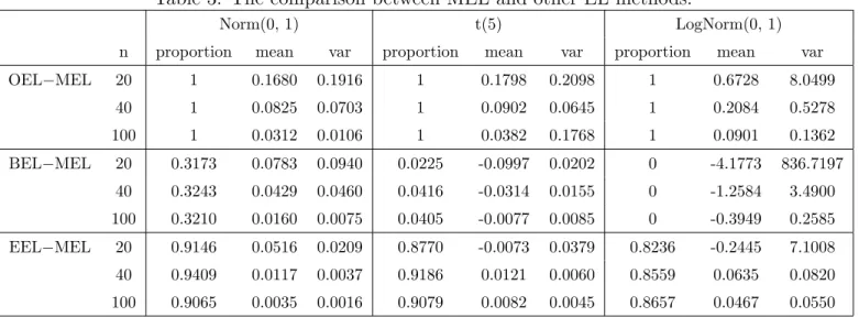
Table 3: The comparison between MEL and other EL methods.
Norm(0,1) t(5) LogNorm(0,1)
n proportion mean var proportion mean var proportion mean var
OEL−MEL 20 1 0.1680 0.1916 1 0.1798 0.2098 1 0.6728 8.0499 40 1 0.0825 0.0703 1 0.0902 0.0645 1 0.2084 0.5278 100 1 0.0312 0.0106 1 0.0382 0.1768 1 0.0901 0.1362 BEL−MEL 20 0.3173 0.0783 0.0940 0.0225 -0.0997 0.0202 0 -4.1773 836.7197 40 0.3243 0.0429 0.0460 0.0416 -0.0314 0.0155 0 -1.2584 3.4900 100 0.3210 0.0160 0.0075 0.0405 -0.0077 0.0085 0 -0.3949 0.2585 EEL−MEL 20 0.9146 0.0516 0.0209 0.8770 -0.0073 0.0379 0.8236 -0.2445 7.1008 40 0.9409 0.0117 0.0037 0.9186 0.0121 0.0060 0.8559 0.0635 0.0820 100 0.9065 0.0035 0.0016 0.9079 0.0082 0.0045 0.8657 0.0467 0.0550 The ”proportion” shows the proportion of positive difference. OEL is LO(θ
0), BEL isLB(θ0), MEL
isLM(θ
0) and EEL isLE(θ0)
For further study of the difference of these EL method, we get the following Table 3, which shows the difference of log-empirical likelihood ratio between MEL and other EL methods. From this table, we can further understand the reason why MEL performs similar as EEL. The difference, LE(θ
0)− LM(θ0), is very small (see the last row and the column ‘mean’ for all three distributions; the mean differences are very small). For the heavy tail distribution LogNorm(0,1), we clearly have (see the column ‘proportion - proportion of positive difference’)
LB(θ
0)<LM(θ0)<LO(θ0).
It implies that for large kurtosis, MEL will correct the empirical likelihood automati-cally, but BEL makes the empirical likelihood too small due to a large Bartlett correc-tion factor b.
3.2
Example II: Regression Models
In this section, we consider the linear regression modelYi =β0+β1xi+εi, whereεis are
independent random variables with mean zero and finite variance and the parameters of interest are (β0, β1). Therefore the estimating equations are
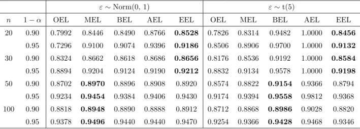
Table 4: Coverage probabilities for regression parameters with homoscedastic error ε.
ε∼Norm(0,1) ε∼t(5)
n 1−α OEL MEL BEL AEL EEL OEL MEL BEL AEL EEL 20 0.90 0.7992 0.8446 0.8490 0.8766 0.8528 0.7826 0.8314 0.9482 1.0000 0.8456 0.95 0.7296 0.9100 0.9074 0.9396 0.9186 0.8506 0.8906 0.9700 1.0000 0.9132 30 0.90 0.8324 0.8662 0.8618 0.8686 0.8656 0.8176 0.8536 0.9192 1.0000 0.8584 0.95 0.8894 0.9204 0.9124 0.9190 0.9212 0.8832 0.9134 0.9578 1.0000 0.9198 50 0.90 0.8702 0.8970 0.8896 0.8908 0.8920 0.8574 0.8822 0.9154 0.9366 0.8794 0.95 0.9234 0.9454 0.9384 0.9406 0.9430 0.9174 0.9394 0.9558 0.9812 0.9368 100 0.90 0.8818 0.8948 0.8890 0.8888 0.8912 0.8712 0.8868 0.8986 0.9028 0.8820 0.95 0.9378 0.9496 0.9440 0.9440 0.9470 0.9254 0.9366 0.9428 0.9468 0.9346
Two different scenarios are considered here: the homoscedastic case and the het-eroscedastic case.
SCENARIO 1: Homoscedasticity
The true parameter values are β0 = 1, β1 = 2 and x is generated from standard uniform distribution. We consider two different types of errors εi, one is drawn from
Norm(0, 1) and the other is a heavy tail distribution t(5). Table 4 shows the coverage probabilities of confidence intervals derived from MEL, OEL, BEL , AEL and EEL under different sample sizesn= 20, 30, 50. Each entry in the Table 4 is based on 5000 random replicates of size n.
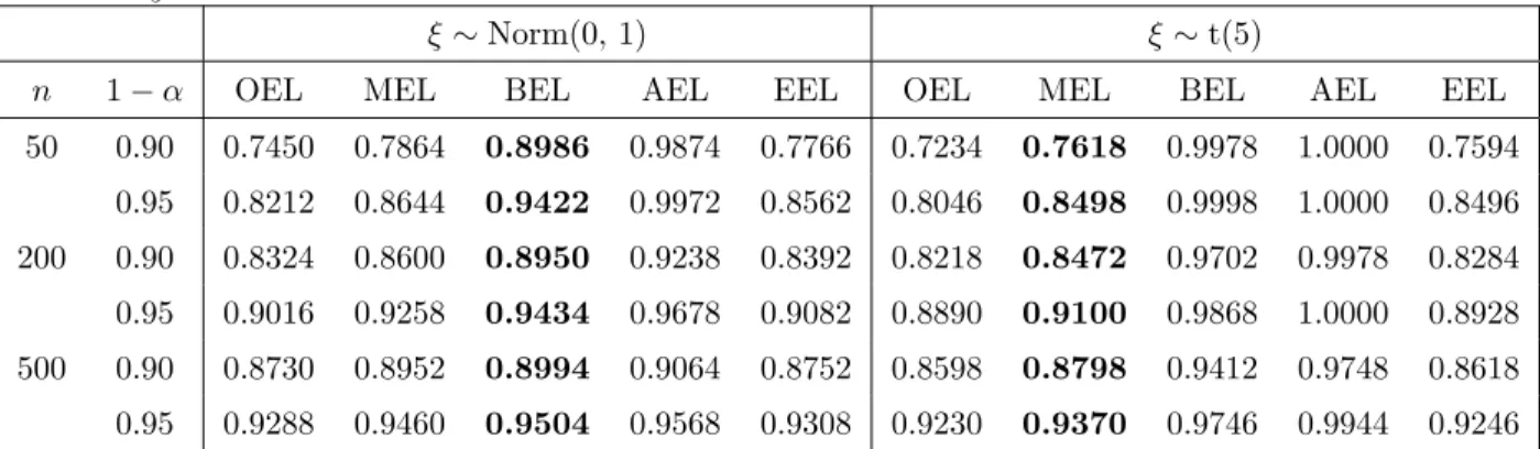
SCENARIO 2: Heteroscedasticity
In this scenario, we explore the performance of MEL ratio statistics under het-eroscedasticity. We choose the true parameter values β0 = 3, β1 = 2, and generate x from Norm(2,3) distribution. We set εi = x2i ∗ξi, and generate ξi from Norm(0,1)
and heavy tail distribution t(5), respectively. Similarly as Scenario 1, we still use the theoretical Bartlett correction constantb to construct confidence regions. In this simu-lation, we choosen = 50, 200, 500 respectively and all results are based on 5000 Monte Carlo replications. The simulation results are summarized in Table 5.
Apart from the similar observations as Example I, we can also get the following observations based on Table 4 and 5,
(1) Homo case: The AEL statistic suffers from a boundedness problem which may lead to 100% confidence regions. For the heavy tail distribution t(5), the BEL
Table 5: Coverage probabilities for regression parameters with heteroscedastic error
ε=x2ξ.
ξ∼Norm(0, 1) ξ∼t(5)
n 1−α OEL MEL BEL AEL EEL OEL MEL BEL AEL EEL 50 0.90 0.7450 0.7864 0.8986 0.9874 0.7766 0.7234 0.7618 0.9978 1.0000 0.7594 0.95 0.8212 0.8644 0.9422 0.9972 0.8562 0.8046 0.8498 0.9998 1.0000 0.8496 200 0.90 0.8324 0.8600 0.8950 0.9238 0.8392 0.8218 0.8472 0.9702 0.9978 0.8284 0.95 0.9016 0.9258 0.9434 0.9678 0.9082 0.8890 0.9100 0.9868 1.0000 0.8928 500 0.90 0.8730 0.8952 0.8994 0.9064 0.8752 0.8598 0.8798 0.9412 0.9748 0.8618 0.95 0.9288 0.9460 0.9504 0.9568 0.9308 0.9230 0.9370 0.9746 0.9944 0.9246
and AEL coverage probabilities are much larger than nominal levels when sample size is small. MEL has the similar performance as EEL, but the coverage errors of MEL is smaller than EEL when sample size increases to n = 50.
(2) Hetero case: All of the coverage probabilities slowly converge to the nominal levels. When sample size n = 500, the coverage probabilities of OEL are still smaller than nominal levels. Under Norm distribution, theoretical BEL performs best; but for the same reason as Example I, under t distribution, both BEL and AEL are much larger. In this case, MEL performs better than EEL uniformly, especially for t distribution.
3.3
Example III: Two Sample Comparison
In this section, we report a simulation study designed to evaluate the performance of the MEL confidence regions proposed in Section 2.2. For simplicity, we consider
d= 1 and g(x) =x. Simulated data sets of various n1 and n2 are generated under the following two scenarios: (1) X drawn from the standard exponential distribution and
Y from χ2(3) distribution; (2) X from t(5) distribution and Y from Log-Norm(0,1) distribution. The nominal coverage levels under consideration are α = 0.90, 0.95. Table 6 shows the coverage percentage comparisons for constructing the confidence intervals, where all results are based on 5000 Monte Carlo replicates. In all cases, the MEL works uniformly better than OEL, and it is much more accurate when sample sizes are small.
Table 6: Coverage probabilities for two sample comparison.
X ∼Exp(1), Y ∼χ2(3) X ∼t(5), Y ∼LogN(0,1)
0.90 0.95 0.90 0.95
(n1, n2) OEL MEL OEL MEL (n1, n2) OEL MEL OEL MEL
(10, 10) 0.8459 0.8836 0.8993 0.9356 (20, 20) 0.8586 0.8793 0.9238 0.9376 (10, 20) 0.8659 0.8835 0.9177 0.9357 (20, 50) 0.8670 0.9123 0.9270 0.9582 (10, 30) 0.8791 0.9074 0.9308 0.9580 (20, 100) 0.8799 0.9253 0.9219 0.9627 (20, 10) 0.8376 0.8903 0.8973 0.9440 (50, 20) 0.8417 0.8806 0.8988 0.9312 (20, 20) 0.8752 0.8976 0.9321 0.9491 (50, 50) 0.8490 0.8800 0.9120 0.9350 (20, 30) 0.8823 0.8936 0.9307 0.9429 (50, 100) 0.8810 0.8878 0.9330 0.9389 (30, 10) 0.8378 0.8921 0.8976 0.9432 (100, 20) 0.8298 0.8718 0.8859 0.9354 (30, 20) 0.8737 0.9023 0.9249 0.9454 (100, 50) 0.8430 0.8758 0.9050 0.9343 (30, 30) 0.8782 0.8942 0.9344 0.9466 (100, 100) 0.8770 0.8840 0.9310 0.9350 (50, 20) 0.8573 0.8931 0.9195 0.9458 (200, 50) 0.8450 0.8756 0.9050 0.9455 (50, 30) 0.8810 0.9030 0.9332 0.9513 (200, 100) 0.8860 0.9013 0.9470 0.9587 (50, 50) 0.8878 0.8987 0.9388 0.9479 (200, 200) 0.8970 0.8990 0.9490 0.9510
3.4
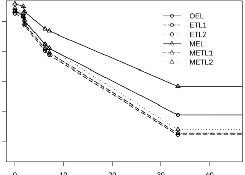
Example IV: Exponentially Tilted Empirical Likelihood
To assess the performance of MEL based on Theorem 2.3, we first carry out the fol-lowing simulation study. We fixed the nominal levelα= 0.95 and sample sizen = 100. The following distributions are considered, Normal(0,1), Weibull(2,1), Generalized Pareto(1/4,1,0) and LNi for LogNorm(0, i2/4), i = 1,2, 3. The skewnesses of these distributions are: 0, 2, 7.07, 1.75, 6.18 and 33.47. Under all these distributions, we implement the following six different methods, (1) OEL, (2) ETL-1: the Newey-Smith empirical entropy difference T1(θ), (3) ETL-2: Jaynes empirical entropy differenceT2(θ), (4) MEL, (5) METL-1: the Newey-Smith mean empirical entropy difference
TM
1 (θ) and (6) METL-2: the Jaynes mean empirical entropy difference T2M(θ).
The results of coverage probabilities based on 5000 Monte Carlo replicates are shown in Figure 3.4 (details can be found in the supplementary file). For all cases, the performance of MEL is the best. Also note that as the skewness increases, MEL becomes much better than other methods. Since Exponential Tilted EL is not Bartlett correctable, see Jing (1996). MEL provides a good way to improve the accuracy of coverage probabilities.
● ● ● ● ● ● 0 10 20 30 40 0.86 0.88 0.90 0.92 0.94 skewness Nominal le v el = 95% ● ● ● ● ● ● ● ● ● ● ● ● ● ● ● OEL ETL1 ETL2 MEL METL1 METL2
Figure 1: Coverage probabilities of mean under different distributions when sample size is 100. Notation ◦ stands for EL-type coverage probabilities and Mfor MEL-type coverage probabilities.
Table 7: Boston Housing Study: confidence intervals for the mean parameter
OEL ETL-1 ETL-2 MEL METL-1 METL-2
(2.9611, 4.4970) (2.9211, 4.4188) (2.9204, 4.4197) (2.9599, 4.5343) (2.9205, 4.4198) (2.9193, 4.4215)
4
Real Data Analysis
In this section, we compare our proposed methods with existing methods using a real dataset. This example is taken from the Boston Housing Study, to illustrate our proposed MEL for Exponentially Tilted Likelihood method in Section 2.3. The distribution of per capita crime rate by town (CRIM) in the dataset follows an unknown heavy-tailed distribution. The data set, which has even been analyzed by Harrison and Rubinfeld (1978), consists of 506 observations. We are interested in the mean of CRIM,
θ. A comparison of OEL, ETL-1, ETL-2, MEL, METL-1 and METL-2 was carried out. The 95% confidence intervals are list in Table 7., which show similar performance of our proposed methods and other existing methods.
5
Conclusion
This paper developed a mean empirical likelihood approach, which gives much more accurate confidence region estimates and coverage probabilities. We presented the method and proved its large sample properties under different application problems, regression models, two-sample comparisons and exponentially tilted likelihood. This new approach outperforms existing methods, in particular for heavy-tail or highly-skewed distributions.
The new method gains its advantage by using the pairwise-mean data and is equivalent to using each data point more than once. A well-known example is the Hodges-Lehmann sign-based estimator, see Hodges and Lehmann (1963), using a sim-ilar mean-pair data idea, which provides much more reliable nonparametric estimators than standard median estimator. Such mean-pair data approach will not be very useful for standard estimation approaches where observations have the same weights, how-ever, it brings new insights to the area of empirical likelihood which assigns different weights for observations. We are currently working on a more general approach of
con-structing such pseudo dataset, which can determine the percentage of pairwise mean data and the percentage of multiple mean data in the pseudo dataset and provide an optimum solution.
Note that Wood et al. (1996) proposed a novel sequential linearization method for empirical likelihood with nonlinear constraints, which can be applied to solve the U-statistics problem in OEL. But from the practical viewpoint, this method typically requires iterations to get satisfactory results. The Jackknife Empirical Likelihood(JEL) method (Jing et al., 2009) can improve the computational efficiency for the sequential linearization method in some degree, but it still needs bootstrap calibrations to improve the performance on coverage probabilities. Our MEL approach uses U-statistics as well, however, it is actually different from the sequential linearization method. In our MEL approach, each pair-wise mean data point Wk = (Vi +Vj)/2 corresponds to a weight pk, k = 1,· · ·, N. On the contrary, in the sequential linearization method, each
pair-wise mean data point (Vi+Vj)/2 corresponds to the productpipj, i, j = 1,· · · , n. This
is why the sequential linearization method has non-linear constraints and involves a heavier computational cost. It is interesting to study how well MEL performs for EL with non-linear constraints and we left this to future research.
A
Proof of Theorem 2.1
Denote Vi = Vi(θ0) and Wi = Wi(θ0). We shall introduce the following lemma, which is a key for the proof of Theorem 2.1.
Lemma A.1.
Under the condition Cov(V1) = Σ exists, rank(Σ) = d, we have(i) max 1≤k≤NkWkk=op(n 1/2), (ii) e0 1 N N X k=1 Wk !
=Op(n−1/2), where e is any unit vector in Rd,
(iii) 1 N N X k=1 WkW0k = 1 2Σ+op(1), (iv) 1 N N X k=1 W0kWk =Op(1).
Proof. (i) Since Cov(Vi) =Σexists, we immediately have maxikVik=op(n1/2) and max 1≤k≤NkWkk= maxi≤j Vi+Vj 2 ≤ 1 2 max i kVik+ maxj kVjk =op(n1/2). (ii) Noticing 1 N N X k=1 Wk = 1 2N n X i=1 n X j=1 Vi+Vj 2 + n X i=1 Vi ! = n+ 1 2N n X i=1 Vi = ¯Vn,
and following the assumption Cov(V1) =Σ, we can obtain e0V¯n = e0(1nPni=1Vi) = Op(n−1/2). Therefore e0 1 N N X k=1 Wk ! =Op(n−1/2). (iii) 1 N N X k=1 WkW0k = 1 2N n X i=1 n X j=1 Vi+Vj 2 Vi+Vj 2 0 + n X i=1 ViV0i ! = 1 2(n+ 1) 1 √ n n X i=1 Vi ! 1 √ n n X i=1 V0i ! + n+ 2 2(n+ 1) 1 n n X i=1 ViV0i ! = 1 2Σ+op(1). (iv) 1 N N X k=1 kWkk2 = n+ 2 2(n+ 1) 1 n n X i=1 V0iVi ! + 1 2(n+ 1) 1 √ n n X i=1 V0i ! 1 √ n n X i=1 Vi ! =Op(1).
Now we can prove Theorem 2.1.
Proof. According to Lemma 11.1 in Owen (2001), with probability tending to 1, 0 is inside the convex hull of Wk, k = 1,2,· · · , n. By using the Lagrange multiplier, we
have
pk=
1
N(1 +λ0Wk) >0,
where λ satisfies the equationP
pkWk = 1. Then applying Lemma A.1, we have
On the other hand, with following equation 0 = 1 N N X k=1 Wk 1 +λ0Wk = 1 N N X k=1 Wk− 1 N N X k=1 WkW0k ! λ+ 1 N N X k=1 Wk(λ0Wk)2 1 +λ0Wk ,
equation((A.1)) and Lemma A.1, we get
λ= N X k=1 WkW0k !−1 N X k=1 Wk ! +op(n−1/2).
Using Taylor’s expansion, we can write
LM(θ 0) = 2 n+ 1 N X k=1 log(1+λ0Wk) = 2 n+ 1 N X k=1 λ0Wk− 1 2(λ 0 Wk)2 + rN n+ 1, (A.2) where krNk ≤Ckλk3 max 1≤k≤NkWkk N X k=1 kWkk2 =Op(n−3/2)op(n1/2)Op(n2) =op(n).
Substitute λ into ((A.2)), we obtain
LM(θ 0) = 1 n+ 1 N X k=1 Wk ! N X k=1 WkW0k !−1 N X k=1 Wk ! +op(1) = 2N n+ 1 ¯ V0nΣ−1V¯n+op(1) =nV¯ 0 nΣ −1¯ Vn+op(1)→χ2(d), in dist.
B
Proof of Theorem 2.2
The notations follow that in Section 2.2. First we shall introduce the following Lemma giving the relation of λ1, λ2 and µ.
Lemma B.1.
Assume ΣX := Cov(X) and ΣY :=Cov(Y) exist and rank(ΣX) = rank(ΣY) =d. Denote µ0 as the mean of X andVX = 1 2δΣX, VY = 1 2(1−δ)ΣY, CX = 1 N δ N1 X s=1 (WXs −µ0), CY = 1 N(1−δ) N2 X t=1 (WYt −µ0). Then we have (i) λ1 = (VX)−1(CX −µ) +op(n−1/2), λ2 = (VY)−1(CY −µ) +op(n−1/2),
µ=VX (VX +VY) −1 VY V−X1CX +V−Y1CY =µ0+Op(n−1/2), (ii) SX = 1 N1 N1 X s=1 (WXs −µ)(WXs −µ)T = 1 2ΣX +op(1), SY = 1 N2 N2 X t=1 (WYt −µ)(WYt −µ)T = 1 2ΣY +op(1).
The proof of Lemma B.1 is similar to Liu et al. (2008) and is omitted here. Now we provide the proof of Theorem 2.2.
Proof. Using Taylor’s expansion, we can write
LM 2 (θ0) = 2 n N1 X s=1 log1 +δ−1λ01(WXs −µ)+ 2 n N2 X t=1 log1 + (1−δ)−1λ02(WYt −µ)+ rN n ,
With a similar argument as that in Theorem 2.1, we know thatrN is of orderop(n−1).
Therefore we have LM 2 (θ0) = 2 n N1 X s=1 δ−1λ01(WXs −µ)− 1 n N1 X s=1 δ−1λ01(WXs −µ)2 +2 n N2 X t=1 (1−δ)−1λ02(WYt −µ)− 1 n N2 X t=1 (1−δ)−1λ02(WYt −µ)2 +op(1) = 2N1 n δ −1λ0 1(CX +µ0−µ)− N1 n δ −1λ0 1SXδ−1λ1 +2N2 n (1−δ) −1 λ02(CY +µ0−µ)− N2 n (1−δ) −1 λ02SY(1−δ)−1λ2+op(1).
Substituting (λ1, λ2) intoLM2 (θ0) and with some simple calculations, we further obtain
LM
2 (θ0) = 2n−1N δ(CX −µ)0Σ−X1(CX −µ) + 2n−1N(1−δ)(CY −µ)0Σ−Y1(CY −µ)
+n−1N(CX −µ)0VX−1+ (CY −µ)0V−Y1
µ0+op(1).
Since (CX −µ)0V−X1+ (CY −µ)0V−Y1 = 0, we can rewrite the aboveLM2 (θ0) as
LM 2 (θ0) = 2n−1N δ(CX −µ)0Σ−X1(CX −µ) + 2n−1N(1−δ)(CY −µ)0Σ−Y1(CY −µ) +op(1) = n−1N(CX −CY)0(VX +VY)−1(CX −CY) +op(1) = n(CX −CY)0 1 ∆2ΣX + 1 (1−∆)2ΣY −1 (CX −CY) +op(1). (B.1)
Noting that CX −CY = ¯X −Y¯, we then apply the Central Limit Theorem and
have (CX −CY)0 1 n1 ΣX + 1 n2 ΣY −1 (CX −CY)
= n(CX −CY)0 1 ∆ΣX + 1 1−∆ΣY −1 (CX −CY)→χ2(d). (B.2)
The theorem is then proved by the fact that equations ((B.1)) and ((B.2)) together imply n−1LM2 (θ0)→ d X k=1 rkχ2k(1), in dist.
where χ2k(1) are standard χ2 distribution, and rk are the eigenvalues of (RM)−1R,
R= 1 ∆0 ΣX + 1 1−∆0 ΣY, RM = 1 ∆2 0 ΣX + 1 (1−∆0)2 ΣY.
C
Proof of Theorem 2.4
Proof. Denote ρ1 = dρ(v)/dv, ρ2 = d2ρ(v)/dv2, and Γk(θ) = ∂Wk(θ)/∂θ.
Under the assumptions A1-A5, similarly as proof of Theorem 2.2 and 3.1 in Newey and Smith (2004), GMEL estimator ˆθ and the corresponding ˆλ= ˆλ(ˆθ) satisfy
N X k=1 ρ1( ˆλ T Wk(ˆθ)) ∂Wk(θ) ∂θ θ=ˆθ T ˆ λ=0, N X k=1 ρ1( ˆλTWk(ˆθ))Wk(ˆθ) = 0, and ˆ θ→θ0, λˆ =Op(n−1/2).
By Taylor expansion for (ˆθT, λˆT)T at (θT
0, 0)T, 0 0 = 0 −1 N PN k=1Wk(θ0) +ΨN ˆ θ−θ0 ˆ λ−0 , (C.1) where ΨN is a (d+m)∗(d+m) matrix, ΨN = 1 N 0, PNk=1ρ1( ˜λ T Wk(˜θ))ΓTk(˜θ) PN k=1ρ1( ˜λ T Wk(˜θ))Γk(˜θ) PN k=1ρ2( ˜λ T Wk(˜θ))WTk(˜θ)Wk(˜θ) ,
˜
θ and ˜λ are vectors between (ˆθT, λˆT)T and (θT
0, 0)T. Since ρ1(0) =−1, ρ2(0) =−1, together with Lemma A1 in Newey and Smith (2004), we get
max k |ρ1( ˜λ T Wk(˜θ) + 1| →0, in pr. max k |ρ2( ˜λ T Wk(˜θ) + 1| →0, in pr.
Further, using the similar proof as Lemma A.1 in Appendix A, we have 1 N N X k=1 ρ1( ˜λ T Wk(˜θ))Γk(˜θ) =−Γ0+op(1), 1 N N X k=1 ρ2( ˜λ T Wk(˜θ))WTk(˜θ)Wk(˜θ) =− 1 2Σ0+op(1). (C.2) Hence ΨN →Ψ= 0, −ΓT 0 −Γ0 −12Σ0 , Ψ −1 = 1 2K, −L −LT −2H , where K = (ΓT0Σ−01Γ0)−1, L=KΓT0Σ −1 0 , H =Σ −1 0 −Σ −1 0 Γ0KΓT0Σ −1 0 . Denote ¯W(θ) = N−1PN k=1Wk(θ). Since ¯W(θ0) =n−1 Pn i=1Vi(θ0) = Op(n−1/2),
after solving equation (C.1), we get
√ n ˆ θ−θ0 ˆ λ−0 = −Ψ −1 N √ n 0 −W¯ (θ0) = Ψ −1 0 √ nW¯ (θ0) +op(1) = −L√nW¯ (θ0) −2H√nW¯ (θ0) +op(1). Therefore 1 N N X k=1 Wk(ˆθ) ! = 1 N N X k=1 Wk(θ0) ! − 1 N N X k=1 Γk(˜θ) ! (ˆθ−θ0) = (I−Γ0L) 1 N N X k=1 Wk(θ0) ! =−1 2Σ0λˆ+op(n −1/2). (C.3)
Using Taylor expansion, 1 N N X k=1 ρ( ˆλTWk(ˆθ)) = ρ0−λˆ T 1 N N X k=1 Wk(ˆθ) ! + 1 2 ˆ λT 1 N N X k=1 ρ2( ˜λ T Wk(ˆθ))Wk(ˆθ)WTk(ˆθ) ! ˆ λ
where ˜λ is between ˆλ and 0, and (C.2), we have 1 N N X k=1 ρ( ˆλTWk(ˆθ)) = ρ0−λˆ T ¯ W(ˆθ)−1 4 ˆ λTΣ0λˆ +op(n−1) = ρ0+ ¯W T (ˆθ)Σ−01W¯ (ˆθ) +op(n−1) = ρ0+ 1 n n X i=1 Vi(ˆθ) !T Σ−01 1 n n X i=1 Vi(ˆθ) ! +op(n−1).
It follows Newey and Smith (2004) that
n 1 n n X i=1 Vi(ˆθ) !T Σ−01 1 n n X i=1 Vi(ˆθ) ! →χ2(m−d), in dist. Hence n 1 N N X k=1 ρ( ˆλTWk(ˆθ))−ρ0 ! →χ2(m−d), in dist.
References
Chen, S. (1993). On the Accuracy of Empirical Likelihood Confidence Regions for
Linear Regression Model. Annals of the Institute of Statistical Mathematics. 45, 621–637.
Chen, J.,Variyath, A.M.&Abraham, B.(2008). Adjusted Empirical Likelihood
and its Properties. Journal of Computational Graphical Statistics. 17, 426–443.
Corcoran, S. A. (1998). Bartlett Adjustment of Empirical Discrepancy Statistics.
Biometrika. 85(4), 967–972.
DiCiccio, T., Hall, P. & Romano, J. (1991). Empirical Likelihood is
Bartlett-correctable. Annals of Statistics. 19, 1053–1061.
Hall, P. & La Scala, B. (1990). Methodology and Algorithm of Empirical
Likeli-hood. International Statistical Review. 58, 109–127.
Harrison, D.&Rubinfeld, D.L.(1978). Hedonic Prices and the Demand for Clean
Hodges, Jr. J.L.& Lehmann, E.L. (1963). Estimates of Location Based on Rank
Tests. The Annals of Mathematical Statistics.34, 598–611.
Jaynes, E.T. (1982). On the Rational of Maximum Entropy Methods. Proceedings
of IEEE International Conference.70, 939–952.
Jing B.Y.(1996). Exponential Empirical Likelihood is Not Bartlett Correctable.
An-nals of Statistics 24, 365–369.
Jing B.Y. Yuan J. & Zhou W.(2009). Jackknife Empirical Likelihood. Journal of
the American Statistical Association.104, 1224–1232.
Liu, Y.&Chen, J.(2010). Adjusted Empirical Likelihood with High-order Precision.
Annals of Statistics.38, 1341–1362.
Liu, Y., Zou, C. & Zhang, R. (2008). Empirical Likelihood for the Two-sample
Mean Problem. Statistics and Probability Letters. 78, 548–556.
Newey, W.K.&Smith, R.J.(2004). Higher Order Properties of GMM Generalized
Empirical Likelihood Estimators. Econometrica, 72, 219–255.
Owen, A. B. (1990). Empirical Likelihood Ratio Confidence Regions. Annals of
Statistics.18, 90–120.
Owen, A. B. (2001). Empirical Likelihood. Chapman and Hall, London.
Qin, J. & Lawless, L. (1994). Empirical Likelihood and General Estimating
Equa-tions. Annals of Statistics. 22, 300–325.
Rao J.N. K.&Scott A. J.(1981). The Analysis of Categorical Data from Complex
Sample Surveys: Chi-Squared Tests for Goodness of Fit and Independence in Two-Way Tables. Journal of the American Statistical Association.76, 221–230.
Tsao, M.(2004). Bounds on Coverage Probabilities of the Empirical Likelihood Ratio
Confidence Regions. Annals of Statistics.32, 1215–1221.
Tsao, M. & Wu, F. (2013). Empirical Likelihood on the Full Parameter Space.
Wood, A.T., Do, K.A.&Broom, B.M. (1996). Sequential linearization of
empiri-cal likelihood constraints with application to U-statistics. Journal of Computational and Graphical Statistics. 54, 365–85.
Xue L.G. & Wang Q.H.(2012). Empirical likelihood for single-index