Empirical Likelihood Methods for
Pretest-Posttest Studies
by
Min Chen
A thesis
presented to the University of Waterloo in fulfillment of the
thesis requirement for the degree of Doctor of Philosophy
in Statistics
Waterloo, Ontario, Canada, 2015
c
I hereby declare that I am the sole author of this thesis. This is a true copy of the thesis, including any required final revisions, as accepted by my examiners.
Abstract
Pretest-posttest trials are an important and popular method to assess treatment effects in many scientific fields. In a pretest-posttest study, subjects are randomized into two groups: treatment and control. Before the randomization, the pretest responses and other baseline covariates are recorded. After the randomization and a period of study time, the posttest responses are recorded. Existing methods for analyzing the treatment effect in pretest-posttest designs include the two-sample t-test using only the posttest responses, the paired t-test using the difference of the posttest and the pretest responses, and the analysis of covariance method which assumes a linear model between the posttest and the pretest responses. These methods are summarized and compared by Yang and Tsiatis (2001) under a general semiparametric model which only assumes that the first and second moments of the baseline and the follow-up response variable exist and are finite. Leon et al. (2003) considered a semiparametric model based on counterfactuals, and applied the theory of missing data and causal inference to develop a class of consistent estimator on the treatment effect and identified the most efficient one in the class. Huang et al. (2008) proposed a semiparametric estimation procedure based on empirical likelihood (EL) which incorporates the pretest responses as well as baseline covariates to improve the efficiency.
The EL approach proposed by Huang et al. (2008) (the HQF method), however, dealt with the mean responses of the control group and the treatment group separately, and the confidence intervals were constructed through a bootstrap procedure on the conven-tional normalized Z-statistic. In this thesis, we first explore alternative EL formulations that directly involve the parameter of interest, i.e., the difference of the mean responses between the treatment group and the control group, using an approach similar to Wu and Yan (2012). Pretest responses and other baseline covariates are incorporated to impute the potential posttest responses. We consider the regression imputation as well as the non-parametric kernel imputation. We develop asymptotic distributions of the empirical likelihood ratio statistic that are shown to be scaled chi-squares. The results are used to construct confidence intervals and to conduct statistical hypothesis tests. We also derive
the explicit asymptotic variance formula of the HQF estimator, and compare it to the asymptotic variance of the estimator based on our proposed method under several scenar-ios. We find that the estimator based on our proposed method is more efficient than the HQF estimator under a linear model without an intercept that links the posttest responses and the pretest responses. When there is an intercept, our proposed model is as efficient as the HQF method. When there is misspecification of the working models, our proposed method based on kernel imputation is most efficient.
While the treatment effect is of primary interest for the analysis of pretest-posttest sample data, testing the difference of the two distribution functions for the treatment and the control groups is also an important problem. For two independent samples, the non-parametric Mann-Whitney test has been a standard tool for testing the difference of two distribution functions. Owen (2001) presented an EL formulation of the Mann-Whitney test but the computational procedures are heavy due to the use of a U-statistic in the constraints. We develop empirical likelihood based methods for the Mann-Whitney test to incorporate the two unique features of pretest-posttest studies: (i) the availability of base-line information for both groups; and (ii) the missing by design structure of the data. Our proposed methods combine the standard Mann-Whitney test with the empirical likelihood method of Huang, Qin and Follmann (2008), the imputation-based empirical likelihood method of Chen, Wu and Thompson (2014a), and the jackknife empirical likelihood (JEL) method of Jing, Yuan and Zhou (2009). The JEL method provides a major relief on computational burdens with the constrained maximization problems. We also develop bootstrap calibration methods for the proposed EL-based Mann-Whitney test when the corresponding EL ratio statistic does not have a standard asymptotic chi-square distri-bution. We conduct simulation studies to compare the finite sample performances of the proposed methods. Our results show that the Mann-Whitney test based on the Huang, Qin and Follmann estimators and the test based on the two-sample JEL method perform very well. In addition, incorporating the baseline information for the test makes the test more powerful.
Finally, we consider the EL method for the pretest-posttest studies when the design and data collection involve complex surveys. We consider both stratification and inverse probability weighting via propensity scores to balance the distributions of the baseline covariates between two treatment groups. We use a pseudo empirical likelihood approach to make inference of the treatment effect. The proposed methods are illustrated through an application using data from the International Tobacco Control (ITC) Policy Evaluation Project Four Country (4C) Survey.
Acknowledgements
First and foremost, I would like to express my deep and sincere gratitude to my PhD supervisors, Dr. Mary E. Thompson and Dr. Changbao Wu, for their patience, kindness, enthusiasm, and immense knowledge. Without their guidance, continuous support and encouragement throughout my PhD study, it would not be possible for me to finish this thesis.
I would also like to thank the members of my thesis committee, Dr. Pengfei Li, Dr. Yingli Qin, Dr. Min Tsao (University of Victoria), and Dr. Suzanne Tyas (School of Public Health and Health Systems, University of Waterloo), for their insightful comments and inspiring questions.
Additionally I wish to thank the faculty members and staff of the Department of Statis-tics and Actuarial Science at the University of Waterloo. I am grateful to Dr. Christian Boudreau for his kind help on SAS programming. I thank Mary Lou Dufton for her will-ingness to help and her excellent administrative support.
I would like to acknowledge the International Tobacco Control Policy Evaluation Project 4 Country Survey team for permitting the access to the data, which is an important sta-tistical application in my thesis. I particularly thank Grace Li for addressing my many questions on the dataset.
I would like to thank my friends and fellow graduate students at Waterloo who gave me continued encouragement and made my life as a PhD student more joyful.
Last but not least, I want to give my very special thanks to Ying Yan for his love, understanding, and endless support.
Dedication
To my dearest parents who always believe in me, love me and support me uncondition-ally.
Contents
List of Tables xviii
List of Figures xix
1 Introduction 1
1.1 Overview . . . 1
1.2 Empirical Likelihood . . . 4
1.3 Empirical Likelihood for Two-Sample Problems . . . 6
1.4 Outline of the Thesis . . . 9
2 An Imputation Based Empirical Likelihood Approach to Pretest-Posttest Studies 11 2.1 Introduction . . . 11
2.2 Notations and the HQF Estimator . . . 12
2.3 Linear Regression Imputation-Based Empirical Likelihood Approach . . . 14
2.4 Kernel Regression Imputation-Based Empirical Likelihood Approach . . . 18
2.5 Efficiency Comparisons Among Alternative EL
Approaches . . . 20
2.6 Simulation Study . . . 23
2.7 A Real Data Analysis . . . 36
2.8 Concluding Remarks . . . 39
2.9 Proofs and Regularity Conditions . . . 40
2.9.1 Lemmas . . . 40
2.9.2 Proof of Theorem 1 . . . 43
2.9.3 Regularity Conditions for Theorem 2 . . . 47
2.9.4 Proof of Theorem 2 . . . 48
3 Mann-Whitney Test with Empirical Likelihood Methods for Pretest-Posttest Studies 51 3.1 Introduction . . . 51
3.2 Methods for Testing the Difference of Distributions of Two Independent Samples . . . 53
3.2.1 Standard Mann-Whitney Test . . . 53
3.2.2 Two-Sample Empirical Likelihood and Mann-Whitney Test . . . 55
3.2.3 Jackknife Empirical Likelihood for Two-Sample U-Statistics . . . . 58
3.2.4 Notations under the Setting of Pretest-Posttest Studies . . . 61
3.3 Adjusted Mann-Whitney Test Based on the HQF Estimators . . . 62
3.4 Empirical Likelihood Based Mann-Whitney Test with Imputation . . . 69
3.5 Two-sample Jackknife EL Method for Mann-Whitney Test . . . 74
3.6 Simulation Studies . . . 78
3.7 Concluding Remarks . . . 82
4 Empirical Likelihood Method for Pretest-Posttest Studies under Com-plex Survey Design 85 4.1 Introduction . . . 85
4.2 Estimator Based on Propensity Score Stratification and Its Variance Esti-mation . . . 89
4.2.1 The Propensity Score and Stratification . . . 89
4.2.2 Estimator of θ . . . 91
4.2.3 Variance Estimations . . . 93
4.3 Propensity Score Weighting and Two-Sample Pseudo EL Method . . . 100
4.4 Application to the ITC 4 Country Survey Data . . . 108
4.4.1 Variables and Data Management . . . 108
4.4.2 Propensity Score Model and Balance Diagnosis . . . 110
4.4.3 Data Analysis . . . 111
4.5 Two-Sample Pseudo EL Method with Imputation for Survey Data . . . 116
4.5.1 Notations . . . 116
4.5.2 Two-Sample Pseudo EL Method . . . 117
4.6 Concluding Remarks . . . 120
5 Summary and Future Research 121 5.1 Summary and Future Research Topics . . . 121
List of Tables
2.1 Inferences on θ under Model (I), ρ= 0.8,θ0 = 0.3 . . . 28
2.2 Inferences on θ under Model (I), ρ= 0.5,θ0 = 0.3 . . . 29
2.3 Inferences on θ under Model (I), ρ= 0.3,θ0 = 0.3 . . . 30
2.4 Inferences on θ under Model (II), ρ= 0.8, θ0 = 0.3 . . . 31
2.5 Inferences on θ under Model (II), ρ= 0.5, θ0 = 0.3 . . . 32
2.6 Inferences on θ under Model (II), ρ= 0.3, θ0 = 0.3 . . . 33
2.7 Comparisons with Model Misspecifications: (I) and (I*) . . . 34
2.8 Comparisons with Model Misspecifications: (II) and (II*) . . . 35
2.9 Treatment effect estimates for 20±5 weeks post randomization CD4 counts for ACTG 175 . . . 39
3.1 Scenario (A): Empirical Power of Testing H0 :F1 =F0 . . . 82
3.2 Scenario (B): Empirical Power of Testing H0 :F1 =F0 . . . 83
3.3 Scenario (C): Empirical Power of Testing H0 :F1 =F0 . . . 83
4.1 Email invited group, gDI503, before propensity score stratification . . . 113
4.2 Email invited group, gDI503, after propensity score stratification . . . 113
4.4 Email invited group, gFR245v, after propensity score stratification . . . 114 4.5 Data analyses separately for the email invitation group and the no email
invitation group . . . 114 4.6 Pseudo two-sample EL method (the email invitation group and the no email
List of Figures
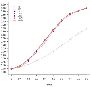
2.1 Power Function of Testing H0 :θ = 0 under Model (I), ρ = 0.8, (n1, n0) =
(50,50) . . . 36 2.2 Power Function of Testing H0 :θ = 0 under Model (II), ρ= 0.8, (n1, n0) =
(50,50) . . . 37 2.3 Power Function of Testing H0 :θ= 0 under Model (I*), (n1, n0) = (200,200) 37
2.4 Power Function of Testing H0 :θ = 0 under Model (II*), (n1, n0) = (200,200) 38
Chapter 1
Introduction
1.1
Overview
Pretest-posttest studies are an important and popular method for assessing treatment effects or the effectiveness of an intervention in many scientific fields, such as medicine, public health and social sciences. In one type of pretest-posttest studies, a random sample of subjects is selected from the target population, and certain baseline (pretest) information is collected for all subjects in the sample. The subjects are then randomly assigned to either the treatment group or the control group. The responses of interest are recorded after a prespecified follow-up time period (posttest) for both groups. The treatment effect is assessed by the difference of the (mean) responses between the two groups. For more traditional pretest-posttest study designs, the responses are measured to all units in the sample at two different time points, one before the treatment (pretest) and the other after the treatment and a prespecified follow-up time (posttest).
There exist several methods in the literature to evaluate the treatment effects in pretest-posttest studies. These methods include (i) the two-sample t-test which directly compares the posttest measurements of two groups ignoring information from the pretest
measure-ments; (ii) the paired t-test comparing the change between the pretest and posttest mea-sures of responses; (iii) the analysis of covariance procedures which impose a linear model on the posttest measures with the treatment indicator and the pretest responses only (ANCOVA I) or the treatment indicator and the pretest measures and their interaction (ANCOVA II) as covariates. Many researchers, such as Brogan and Kutner (1980), Laird (1983), Crager (1987), Stanek (1988), and Follmann (1991), among others, have discussed these approaches under different scenarios but often with specific model assumptions such as normality or equality of variance of pretest and posttest responses.
Yang and Tsiatis (2001) examined some of the above methods under general conditions. They assumed only that the first and second moments of pretest and posttest responses are finite; the conditional joint distribution of the pretest and posttest responses condi-tioning on treatment can be arbitrary. They compared the large sample properties of the treatment effect estimators based on these methods. They also proposed a generalized estimating equation (GEE) method which considers the pretest and posttest measures as a multivariate response, and assumes arbitrary mean and covariance matrix. They showed that all these methods yield consistent and asymptotically normal estimators, and the GEE estimator and the ANCOVA II estimator are asymptotically equivalent and most efficient. In Leon et al. (2003), the authors took a semiparametric perspective without any distributional assumptions, and exploited theory of missing data and causal inference to develop a class of consistent treatment effect estimators and identify the most efficient one in the class. Davidian et al. (2005) later considered the situation when there is missing data in the posttest response.
Huang et al. (2008) proposed a semi-parametric procedure based on the empirical like-lihood (EL) method to estimate the treatment effect in a pretest-posttest study. Their proposed strategy is to use the baseline information to form constraints when maximizing the EL function but estimation of the mean of the posttest response is handled separately for the treatment group and the control group. The treatment effect is then estimated by taking the difference between the two estimated means. They considered scenarios where
posttest responses are subject to missingness, and compared the EL based estimators to the ones in Leon et al. (2003) and to those in Davidian et al. (2005). They found that the EL based estimators achieve the semi-parametric efficiency lower bound under a cor-rectly specified working model which links the posttest response to the pretest response and other baseline covariates; the EL based estimators are more efficient in the semi-parametric sense when a misspecified working model is used to link the posttest response to the pretest response and other baseline covariates.
Although the EL approach proposed in Huang, Qin and Follmann (2008, hereafter referred to as HQF) looks appealing, it seems less natural to estimate the posttest response means for each group separately while the target parameter is actually the difference (i.e., treatment effect). In addition, empirical likelihood ratio confidence intervals or tests for the treatment effect cannot be constructed under the HQF approach. This motivates our proposed EL method for estimating the treatment effect in pretest-posttest studies. There have been considerable research efforts towards the problem of making inference of the treatment effect; however, testing the difference of distributions is rarely studied under the setting of pretest-posttest studies. In this thesis, we also propose the empirical likelihood based methods to test the difference of the distributions of the posttest responses from the treatment group and the control group. Furthermore, we extend our research to the complex survey context. We develop methods for estimating the treatment effect of pretest-posttest studies with observational survey data. Before we present our work, we provide a brief review of the empirical likelihood method in the remainder of this chapter.
The rest of this chapter is organized as follows. In Section 1.2, we briefly review the empirical likelihood (EL) method. In Section 1.3, we summarize the two-sample EL method proposed by Wu and Yan (2012). The outline of the thesis is given in Section 1.4.
1.2
Empirical Likelihood
The method of empirical likelihood (EL) was introduced by Owen (1988), Owen (1990), Owen (2001) for constructing confidence intervals (regions) in nonparametric settings for the mean or other functions of the distribution function. It has become one of the most popular methods in statistical inference over the last 20 years and has applications to many research areas. The empirical likelihood method has many advantages such as data-determined shapes for confidence intervals (regions), ease of incorporation of known con-straints on parameters, Bartlett correctability, and a natural method of combining data from multiple sources. The standard empirical likelihood method for the mean can be demonstrated through the following simple example.
Let {Y1,· · · , Yn} be independent and identically distributed real valued random
vari-ables having a common cumulative distribution functionF(y) with meanµ. Let{y1,· · · , yn}
be a realization of{Y1,· · · , Yn}. The empirical cumulative distribution function ofY1, ..., Yn
is defined as Fn(y) = 1 n n X i=1 I{Yi ≤y}.
It has been shown that Fn uniquely maximizes the nonparametric likelihood L=
Qn
i=1pi,
where pi = F(Yi)−F(Yi−), subject to the constraints
Pn
i=1pi = 1, pi ≥ 0. Moreover,
confidence intervals for µ = E(Y) can be obtained in the following procedure. For any fixedµ, suppose ˆp(µ) = (ˆp1(µ),· · · ,pˆn(µ)) maximizes L=Qni=1pi subject to constraints
n X i=1 pi = 1, pi ≥0, n X i=1 piyi =µ.
Using the Lagrange multiplier method, ˆpi(µ) is given by:
ˆ pi(µ) = 1 n 1 1 +λ(yi−µ) , where the Lagrange multiplierλ is determined by
1 n n X i=1 yi−µ 1 +λ(yi−µ) = 0.
The profile empirical log-likelihood of µis given by lp(µ) =− n X i=1 log{1 +λ(yi−µ)} −nlogn.
The maximum of lp(µ) is attained when µ = ˆµ = n−1Pni=1yi. The profile empirical
likelihood ratio function forµis defined as
R(µ) = max{ Qn i=1pi : Pn i=1pi = 1, Pn i=1piyi =µ, pi ≥0} max{Qn i=1pi : Pn i=1pi = 1, pi ≥0} = max{ n Y i=1 npi : n X i=1 pi = 1, pi ≥0, n X i=1 piyi =µ}. Thus, logR(µ) = lp(µ)−lp(ˆµ) = − n X i=1 log{1 +λ(yi−µ)}.
Owen (2001) proved that−2 logR(µ) has asymptotically aχ2 distribution with one degree
of freedom. This is an important result which is analogous to that for the likelihood ratio statistic under a parametric model, and can be used to test statistical hypotheses and construct confidence intervals for µ.
Since Owen’s pioneer work on empirical likelihood, many other researchers have ex-tended and applied EL to various kinds of statistical problems. Qin and Lawless (1994) linked empirical likelihood to estimating equations, especially when the number of unbiased estimating equations may be greater than the number of parameters. They demonstrated that the EL method can effectively combine unbiased estimating equations and lead to the most efficient estimator. In the context of survey sampling, the EL method has been applied to incorporate auxiliary covariate information to improve efficiency, for example, by Chen and Qin (1993), Wu and Sitter (2001) and Wu and Rao (2006). Recently, the empirical likelihood method has become popular in addressing general missing data problems. Some researchers, such as Wang and Rao (2002) and Liang et al. (2007), first imputed the missing data using a kernel regression function of the observed data and then applied an EL method
to do the statistical inference. For parameters estimation in estimating equations, Wang and Chen (2009) proposed an EL method with non-parametric imputation of missing data. Qin et al. (2009) explored the use of empirical likelihood to effectively combine unbiased estimating equations by separating the complete data unbiased estimating equations from the incomplete data unbiased estimating equations, and their proposed estimators achieve semi-parametric efficiency lower bound when correctly specifying the missing mechanism. Moreover, attention has also been focused on applying the EL to two-sample problems. Jing (1995) showed that the two-sample empirical likelihood for the difference of two pop-ulation means is Bartlett correctable. Qin and Zhang (1997) and Qin (1998) considered a calibration-type empirical likelihood method in the context of the estimation of a response mean in case-control studies. Chen et al. (2003) used a two-sample EL method to combine the complete and incomplete observations under missingness completely at random. Cao and van Keilegom (2009) used an EL-based test to examine whether two populations follow the same distribution. Wu and Yan (2012) developed the weighted EL method with great advantage in computation, a pseudo EL method for comparing two population means when the two samples are selected by complex surveys, a two-sample EL method with missing responses, and bootstrap calibration procedures for the proposed EL methods.
1.3
Empirical Likelihood for Two-Sample Problems
In this section, we review some of the main theories in Wu and Yan (2012). Suppose there are two independent and identically distributed samples{Y11,· · · , Y1n1}, and{Y21,· · · , Y2n2}
fromY1 and Y2 respectively, with E(Y1) =µ1, V ar(Y1) =σ21, and E(Y2) =µ2,V ar(Y2) =
σ22. Let n = n1 +n2. The parameter of interest is θ = µ1 −µ2. Wu and Yan (2012)
de-rived the asymptotic distribution of the standard two-sample empirical log-likelihood ratio statistic on θ. They also proposed the weighted two-sample empirical log-likelihood for-mulation and proved that the weighted two-sample empirical log-likelihood ratio statistic converges to a scaledχ21.
The standard two-sample empirical likelihood function is given by `(p1,p2) = n1 X j=1 log(p1j) + n2 X j=1 log(p2j),
wherep1 = (p11,· · · , p1n1) andp2 = (p21,· · · , p2n2) are the two sets of probability measure
imposed respectively over the two samples. For fixedθ, suppose ˆp1(θ) = (ˆp11(θ),· · · ,pˆ1n1(θ))
and ˆp2(θ) = (ˆp21(θ),· · · ,pˆ2n2(θ)) maximize `(p1,p2) subject to the following constraints:
n1 X j=1 p1j = 1, n2 X j=1 p2j = 1, (1.1) n1 X j=1 p1jY1j − n2 X j=1 p2jY2j =θ . (1.2)
The standard two-sample empirical log-likelihood ratio statistic on θ is defined as r(θ) = n1 X j=1 log(n1pˆ1j(θ)) + n2 X j=1 log(n2pˆ2j(θ)).
In Wu and Yan (2012), the authors showed that
−2r(θ)→−d χ21 as n→ ∞, (1.3)
where “−→d ” denotes convergence in distribution. In the proof of this result, they introduced a nuisance parameter µ0 = µ2 +Op(n−1/2) to facilitate the arguments and rewrote the
constraint (1.2) as n1 X j=1 p1jY1j =µ0+θ and n0 X j=1 p2jY2j =µ0.
The nuisance parameter µ0 serves as a bridge for computing the EL ratio statistic for
θ and will eventually be profiled. By (1.3), the (1− α)-level confidence interval on θ can be constructed as C1 = {θ| − 2r(θ) ≤ χ21(α)}, where χ21(α) is the upper (100α)%
for the Lagrange multiplier, which needs to be calculated based on two samples with an added nuisance parameter µ0. Such difficulty can be avoided through the weighted
empirical likelihood formulation, for which the computation procedures are much simpler and essentially identical to those for one-sample EL problems.
The weighted empirical log-likelihood function is defined as follows: `w(p1,p2) = w1 n1 n1 X j=1 log(p1j) + w2 n2 n2 X j=1 log(p2j),
where w1 = w2 = 1/2. The choice of w1 and w2 is to facilitate the reformulation of
constraints (1.1) and (1.2) into the following equivalent forms:
2 X i=1 wi ni X j=1 pij = 1, (1.4) 2 X i=1 wi ni X j=1 pijuij =0. (1.5)
whereuij =Zij−η,Z1j = (1, Y1j/w1)T,Z2j = (0,−Y2j/w2)T, and η= (w1, θ)T. Suppose
ˆ
pw1j and ˆpw2jmaximize`w(p1,p2) subject to constraints (1.4) and (1.5). Using the standard
Lagrange multiplier method, it can be shown: ˆ
pwij = 1/{ni(1 +λTuij)}, i= 1,2 and j = 1,· · · , ni,
and the Lagrange multiplier λ is the solution to
g(λ) = 2 X i=1 wi ni ni X j=1 uij 1 +λTu ij =0. (1.6)
The weighted two-sample empirical log-likelihood ratio statistic forθ is defined as:
rw(θ) =− 2 X i=1 wi ni ni X j=1 log(1 +λTuij).
Wu and Yan (2012) proved that
−2rw(θ)/c d
−
→χ21 as n→ ∞,
where c is a scaling constant. Based on this result, we can construct confidence intervals and conduct hypothesis testing for θ. The weighted two-sample EL formulation is compu-tationally friendly. It does not involve any nuisance parameters, and the equation (1.6) for the Lagrange multiplier can be solved using the one-sample EL algorithm by Wu (2004).
1.4
Outline of the Thesis
As we discussed in Section 1.1, the method proposed by Huang et al. (2008) for estimating the treatment effect handles the mean responses for the treatment group and the control group separately. Empirical likelihood ratio confidence intervals or tests for the treatment effect cannot be constructed under their approach. In Chapter 2, we propose an alterna-tive EL formulation which directly involves the parameter of interest, i.e., the treatment effect, and incorporates baseline information through an imputation approach. Our focus is to derive the empirical likelihood ratio confidence intervals and tests for the treatment effect under the proposed imputation-based framework. Theoretical results are developed, and finite sample performances of the proposed methods with comparison to existing ap-proaches are investigated through simulation studies. An application to a real data set is also presented.
While the treatment effect, measured as the difference between the two mean responses, is of primary interest, testing the difference of the two distribution functions for the treat-ment and the control groups is also an important problem. The Mann-Whitney test has been a standard tool for testing the difference of distribution functions with two inde-pendent samples. In Chapter 3, we develop empirical likelihood based methods for the Mann-Whitney test to incorporate the two unique features of pretest-posttest studies: (i) the availability of baseline information for both groups; and (ii) the structure of the data
with the missing by design property. Our proposed methods combine the standard Mann-Whitney test with the empirical likelihood method of Huang et al. (2008), the imputation-based empirical likelihood method we proposed in Chapter 2, and the jackknife empirical likelihood method of Jing et al. (2009). Theoretical results are presented and finite sample performances of proposed methods are evaluated through a simulation study.
In Chapter 4, we investigate the EL methods for estimating the treatment effect in pretest-posttest studies with observational survey data. Methods based on propensity score modelling are very popular for making causal inference with observation data. We develop methods based on propensity score stratification and propensity scores weighting for estimating the treatment effect while accommodating the complex survey design. We also study the theoretic properties of our proposed estimators. The proposed methods are illustrated through an application using the data from the International Tobacco Control Four Country Surveys (ITC 4C).
In Chapter 5, we summarize the thesis and discuss some possible future work for the topics that we have studied.
Chapter 2
An Imputation Based Empirical
Likelihood Approach to
Pretest-Posttest Studies
2.1
Introduction
In this chapter, we develop the empirical likelihood based method for making inference of the treatment effect in pretest-posttest studies. Our method has two distinct features: (i) The baseline pretest information is used through a direct model-based imputation proce-dure; and (ii) The EL formulation involves the parameter of interest directly, not the two separate means of responses for the treatment group and the control group. The impu-tation procedure effectively exploits the key feature of the pretest-posttest studies where the responses are missing by design. The EL estimation theory employs the framework of two-sample EL procedures proposed by Wu and Yan (2012) where the EL ratio statistic is formulated directly for the parameter of interest.
The rest of the chapter is organized as follows. In Section 2.2, we introduce some notation and summarize the EL method by Huang et al. (2008). In Section 2.3, we present
our proposed imputation-based two-sample EL estimator for the treatment effect, using a linear model. Our main result is on the asymptotic distribution of the empirical likelihood ratio statistic for the treatment effect. Section 2.4 extends the result when the linear imputation model is replaced by kernel regression. In Section 2.5, we make theoretical comparisons between the efficiencies of the HQF estimator and the imputation-based EL estimators under suitable conditions. Results from a limited simulation study are presented in Section 2.6. An application using a data set from the ACTG 175 study is reported in Section 2.7. Some concluding remarks are given in Section 2.8. Proofs of theoretical results and regularity conditions are given in Section 2.9.
2.2
Notations and the HQF Estimator
Suppose there aren subjects selected from the target population. Measurements on some baseline variables,Z, are taken for allnsubjects. Each subject is then randomly assigned to either the treatment group or the control group, with probabilitiesδand 1−δ respectively. Letn1 be the number of subjects in the treatment group, and n0 =n−n1 be the number
of subjects in the control group. LetRi = 1 if subjectiis assigned to the treatment group
andRi = 0 if subject iis assigned to the control group. Because of the randomization, the
marginal distribution of Z is assumed to be identical for the two groups. Let Y1 and Y0
be the potential posttest responses that a subject would have if assigned to the treatment group and the control group, respectively. Note thatY1will not be observed for any subjects
in the control group and Y0 will not be observed for any subjects in the treatment group.
Hence, the observed data for the treatment group are {(Ri = 1,zi, y1i) : i = 1,· · · , n1},
and the observed data for the control group are {(Ri = 0,zi, y0i) :i=n1+ 1,· · ·, n}. Let
µ1 =E(Y1) andµ0 =E(Y0). The parameter of interest is the treatment effectθ =µ1−µ0.
Huang et al. (2008) proposed to estimate the treatment effect using the empirical likelihood method. However, instead of estimating the treatment effect θ directly, the authors focused on estimatingµ1 andµ0 separately. The HQF estimator of µ1 is computed
as ˆµ1HQF =
Pn1
i=1pˆiy1i, where ˆpiare obtained through the following EL method. Letf(z, y1)
be the joint density function of (Z, Y1) related to the treatment group and f(z) be the
marginal density function of Z. Let pi = f(zi, y1i) for i = 1,· · · , n1 and ri = f(zi) for
i=n1+ 1,· · · , n. The log empirical likelihood function is given by
`= n1 X i=1 log(pi) + n X i=n1+1 log(ri). (2.1)
The ˆpi and ˆri are obtained by maximizing (2.1) subject to pi >0,ri >0 and the following
constraints: n1 X i=1 pi = 1, n X i=n1+1 ri = 1, (2.2) n1 X i=1 pia1(zi) = n X i=n1+1 ria1(zi), (2.3)
where a1(z) = E(Y1|Z = z). It is assumed that E[a1(Z)]2 < ∞. The constraint (2.3) is
the most crucial part for the HQF estimator, since it uses the baseline information from both the treatment group and the control group. The actual form of a1(z) is typically
unknown, but one could use a guessed form, with possible loss of efficiency for the final estimator. The solutions to this constrained maximization problem are given by
ˆ pi = 1 n1 1 1 +λ{a1(zi)−b} , i= 1,· · ·, n1 and ˆri = 1 n0 1 1 +τ{a1(zi)−b} , i=n1+ 1,· · · , n
for a fixed value of b =Pn1
i=1pia1(zi) =
Pn
i=n1+1ria1(zi). The Lagrange multipliers λ and
τ are determined by solving 1 n1 n1 X i=1 a1(zi)−b 1 +λ{a1(zi)−b} = 0 and 1 n0 n X i=n1+1 a1(zi)−b 1 +τ{a1(zi)−b} = 0.
The final value ofb used for computing the ˆpi can be obtained through profiling over the
log empirical likelihood function.
Huang et al. (2008) showed that ˆµ1HQF has the following asymptotic representation:
ˆ µ1HQF = 1 n n X i=1 Riy1i δ −E Y1ψ1(Z)T E ψ1(Z)ψ1(Z)T −1n1 n n X i=1 Ri−δ δ ψ1(zi) o +op n−1/2 ,
whereψ1(z) = (1, a1(z))T. The authors used this asymptotic representation to prove that,
under certain regularity conditions, √n(ˆµ1HQF−µ1)→N(0, σ21), where
σ12 =δ−1E(Y12)−µ21 −(1−δ)δ−1EY1ψ1(Z)T E
ψ1(Z)ψ1(Z)T
−1
EY1ψ1(Z) .
Moreover, the authors showed that ˆµ1HQF is as efficient as the estimator proposed in Leon
et al. (2003) when a1(z) = E(Y1|Z = z) is correctly specified for both methods but the
HQF estimator is more efficient when a misspecifieda1(z) is used for both cases.
Huang et al. (2008) proposed to use the same method to estimate µ0 by ˆµ0HQF, with
{y1i, i= 1,· · · , n1} replaced by{y0i, i=n1+ 1,· · · , n}. The same constraint (2.3) is used
where a1(z) is replaced by a0(z) = E(Y0|Z =z). The treatment effect is then estimated
as ˆθHQF = ˆµ1HQF −µˆ0HQF. For confidence intervals or hypothesis tests on θ, the authors
proposed to use a nonparametric bootstrap method to estimate the variance of ˆθHQF. In
Section 2.5, we will provide an explicit form of the asymptotic variance of ˆθHQF. It should
be noted that empirical likelihood ratio tests on the treatment effect θ are not available under the EL approach used by HQF.
An interesting and practically useful observation for the HQF estimator is that, if Z
is univariate and a1(z) = γ0 +γ1z for some unknown γ0 and γ1, the constraint (2.3) is
equivalent to Pn1
i=1pizi =
Pn
i=n1+1rizi under the normalization constraints
Pn1
i=1pi = 1
and Pn
i=n1+1ri = 1.
2.3
Linear Regression Imputation-Based Empirical
Likelihood Approach
In this section, we propose an alternative empirical likelihood approach to inferences for pretest-posttest studies. Our method effectively exploits the two distinct features of the problem: (i) availability of baseline information for all subjects in the studies, and (ii) response variables missing by design. Our formulation of the EL function involves directly
the parameter of interest,θ =µ1−µ0, not the two separate means of the post-test responses.
Our primary objective is to develop the empirical likelihood ratio test for the treatment effect θ.
The two features of pretest-posttest sample data can be better summarized through the following table:
i 1 2 · · · n1 n1+ 1 n1+ 2 · · · n
Z Z1 Z2 · · · Zn1 Zn1+1 Zn1+2 · · · Zn
Y1 Y11 Y12 · · · Y1n1 ∗ ∗ · · · ∗
Y0 ∗ ∗ · · · ∗ Y0(n1+1) Y0(n1+2) · · · Y0n
The complete observations of Z on all subjects provide an opportunity to impute the missing values “∗” of the response variables due to the unique design used for the studies. The imputation-based approach not only uses the baseline information in a more effective way but also produces two samples with enlarged sample sizes. We first consider the following linear regression models for the two response variables Y1 and Y0:
Y1i = ZTi β1+1i, i= 1,· · · , n , (2.4)
Y0i = ZTi β0+0i, i= 1,· · · , n , (2.5)
where β1 and β0 are respectively the regression parameters for the treatment and the control, and 1i’s and 0i’s are independent errors with zero mean and variance σ21 and
σ2
0, respectively. It is assumed for simplicity that both models (2.4) and (2.5) include an
intercept. The case where there is no intercept, discussed in Sections 2.5 and 2.6, can be handled similarly. The two assumed models imply that the missing responses in one group would follow the same model if the subjects were assigned to the other group.
We consider deterministic regression imputation for the missing responses. Let ˆ β1 = Xn i=1 RiZiZTi −1Xn i=1 RiZiY1i, ˆ β0 = n X i=1 (1−Ri)ZiZTi −1Xn i=1 (1−Ri)ZiY0i
be the ordinary least squares estimators forβ1 and β0. Let
Y1∗i =ZTi βˆ1, i=n1+ 1,· · · , n and Y0∗i =Z T
i βˆ0, i= 1,· · · , n1
be respectively the imputed values of Y1 for the subjects in the control group and the
imputed values of Y0 for the subjects in the treatment group. Note that E(ZTi βˆ1) =
E(Y1i) =µ1, andE(ZiTβˆ0) = E(Y0i) = µ0. After the imputation, we obtain two augmented
samples for the two posttest response variables given by
{Y˜1i =RiY1i+ (1−Ri)Y1∗i, i= 1,· · · , n} and {Y˜0i = (1−Ri)Y0i+RiY0∗i, i= 1,· · ·, n}.
We develop a two-sample empirical likelihood method for the parameter of interest θ=µ1−µ0 =E(Y1)−E(Y0), using the formulation described in Wu and Yan (2012). Our
primary objective is to construct an EL test on the treatment effectθ using the empirical likelihood ratio statistic. The log empirical likelihood function is given by
`(p,q) = n X i=1 log(pi) + n X i=1 log(qi), where p = (p1,· · · , pn)T, q = (q1,· · · , qn)T, pi = f(y1i), i = 1,· · · , n, qi = g(y0i), i =
1,· · · , n, and f(·) and g(·) are the marginal density functions for Y1 and Y0. For a fixed
value of θ, let p(θ) = (p1(θ),· · · , pn(θ))T and q(θ) = (q1(θ),· · · , qn(θ))T be the maximizer
of`(p,q) subject to pi >0, qi >0 and the constraints n X i=1 pi = 1, n X i=1 qi = 1, (2.6) n X i=1 piY˜1i− n X i=1 qiY˜0i =θ. (2.7)
There exists a computational algorithm for finding the solution to this constrained max-imization problem for a fixed θ without introducing any additional parameters. See Wu and Yan (2012) for further detail. The maximum EL estimator of θ under the assumed linear models is given by
ˆ θlinEL = 1 n n X i=1 ˜ Y1i− 1 n n X i=1 ˜ Y0i =Y¯˜1−Y¯˜0. (2.8)
We now present one of our major results on the EL ratio statistic on θ. Let ˆp(θ) = (ˆp1(θ),· · · ,pˆn(θ))T and ˆq(θ) = (ˆq1(θ),· · · ,qˆn(θ))T be the maximizer of `(p,q) under the
constraints (2.6) and (2.7) for a fixed θ. Let r(θ) = n X i=1 log (npˆi(θ)) + n X i=1 log (nqˆi(θ))
be the EL ratio statistic on θ. We have the following result regarding the asymptotic distribution ofr(θ).
Theorem 1. Suppose that E(kZk2) < ∞, σ2
1 < ∞, σ20 < ∞ and n1/n → δ ∈ (0,1) as n → ∞. Suppose also that models (2.4) and (2.5) hold. Then −2r(θ)/c1 converges in distribution to a χ2 random variable with one degree of freedom as n → ∞, where
θ =E(Y1)−E(Y0) = µ1 −µ0. The scaling constant c1 is given by c1 ={( ˜V1 + ˜V0)/V}−1, where V = (β1 −β0)TΣ Z(β1 −β0) +δ −1σ2 1 + (1−δ) −1σ2 0, V˜1 = n−1Pin=1( ˜Y1i −µ1)2, ˜
V0 =n−1Pni=1( ˜Y0i−µ0)2, and ΣZ is the variance-covariance matrix of Z.
From the proof of Theorem 1 presented in Section 2.9.2 we see thatV /n is the asymp-totic variance of ˆθELlin. Under the same conditions of the theorem, we have that
√
n(ˆθlinEL−θ)
converges in distribution to N(0, V). Results of Theorem 1 can be used to construct the (1− α)-level EL ratio confidence interval on θ: C1 = {θ | −2r(θ)/ˆc1 ≤ χ21(α)}, where
χ2
1(α) is the upper αquantile of the χ21 distribution and ˆc1 is a consistent estimator of the
scaling constant c1. It can be shown that if ˆc1 is a consistent estimator of c1 such that
ˆ
2.4
Kernel Regression Imputation-Based Empirical
Likelihood Approach
The results presented in Section 2.3 require the validity of the assumed linear regression models (2.4) and (2.5). In this section, we consider nonparametric kernel regression models as a robust alternative. Imputation for missing responses based on a kernel regression model was discussed in Cheng (1994). Wang and Rao (2002) considered the one-sample EL method with kernel regression imputation for missing values. Letm1(z) = E(Y1|Z =z)
and m0(z) = E(Y0|Z = z). We replace the linear regression imputed values Y1∗i =Z T iβˆ1
and Y0∗i = ZTiβˆ0 by kernel regression imputed values ˆm1(Zi) and ˆm0(Zi), respectively.
Cheng (1994) used the following kernel estimators for m1(z) and m0(z):
ˆ m1(z) = n X i=1 RiY1iK((z−Zi)/hn)/ n X i=1 RiK((z−Zi)/hn), (2.9) ˆ m0(z) = n X i=1 (1−Ri)Y0iK((z−Zi)/hn)/ n X i=1 (1−Ri)K((z−Zi)/hn), (2.10)
whereK(·) is a kernel function andhnis a bandwidth sequence which decreases to zero as
n goes to infinity. When the sample sizes are not large enough, neighbourhoods of certain values of z might contain very few observations, which might cause ˆm1(z) or ˆm1(z) to be
very unstable. Wang and Rao (2002) proposed to use the following modified versions of the kernel estimators by first defining
ˆ g1(z) = (nhn)−1 n X i=1 RiK((z−Zi)/hn) and ˆg1bn(z) = max{gˆ1(z), bn}, ˆ g0(z) = (nhn)−1 n X i=1 (1−Ri)K((z−Zi)/hn) and ˆg0bn(z) = max{ˆg0(z), bn}
for a suitably chosen sequencebn, and then replacing ˆm1(z) by ˆm1bn(z) = ˆm1(z)ˆg1(z)/ˆg1bn(z),
ˆ
m0(z) by ˆm0bn(z) = ˆm0(z)ˆg0(z)/ˆg0bn(z).
be imitated under kernel regression imputation if we simply define ˜
Y1keli = RiY1i + (1−Ri) ˆm1bn(Zi), i= 1,2,· · · , n ,
˜
Y0keli = (1−Ri)Y0i+Rimˆ0bn(Zi), i= 1,2,· · · , n .
The maximum EL estimator ofθ under the assumed kernel regression models is given by ˆ θELkel= 1 n n X i=1 ˜ Y1keli − 1 n n X i=1 ˜
Y0keli =Y¯˜1kel−Y¯˜0kel. (2.11)
Letrkel(θ) be defined in the same way as r(θ) is computed in Section 2.3, with ˜Y
1i and ˜Y0i
respectively being replaced by ˜Y1keli and ˜Y0keli .
Theorem 2. Under the conditions C1-C6 specified in Section 2.9.3, −2rkel(θ)/c2 converges in distribution to a χ2 random variable with one degree of freedom when n → ∞ and
θ=µ1−µ0. The scaling constant c2 is given by c2 =Vkel/( ˜V1kel+ ˜V0kel), where
˜ V1kel = n−1 n X i=1 ( ˜Y1keli −µ1)2, V˜0kel = n −1 n X i=1 ( ˜Y0keli −µ0)2, Vkel = V ar(m1(Z)−m0(Z)) +δ−1E(σ21(Z)) + (1−δ) −1E(σ2 0(Z)) with σ2 j(z) =V ar(Yj|Z =z) for j = 1,0.
From the proof of Theorem 2 presented in Section 2.9.4 we see that Vkel/n is the
asymptotic variance of the maximum EL estimator ˆθELkel and
√
n(ˆθELkel−θ) converges in
dis-tribution toN(0, Vkel). A (1−α)-level EL ratio confidence interval onθ can be constructed as C2 = {θ | −2rkel(θ)/ˆc2 ≤ χ21(α)}, where ˆc2 is a consistent estimator of c2 and χ21(α) is
the upperα% quantile of the χ2
1 distribution.
Two of the major issues with kernel regression modelling are the curse of dimensionality and bandwidth selection. The method presented in this section is most helpful when the linear regression models are questionable and the baseline variables Z are of low dimen-sion. In practice, the optimal bandwidth may be difficult to estimate, and the choice of
bandwidth can be determined by a data-dependent cross-validation method. The cross val-idated bandwidth minimizes the sum of squared errors between the data and the estimates from the kernel regression. The procedure of a K-fold cross validation (Hastie et al. (2001)) can be summarized as following: consider a possible set of bandwidths {h1,· · · , hp}. For
each hi, i= 1,· · · , p, we
1. randomly split the data into (roughly)K equal-sized parts for both treatment group and control group;
2. for the kth part (test), fit kernel regression with bandwidth h
i to the other K −1
parts of data (training), and calculate the sum of the squared errors of the fitted values and the true data of the kth part for both groups;
3. repeat number 2 fork= 1,· · ·, K, and then calculate the total sum of squared errors. Repeat the process for i= 1,· · · , p, then the cross-validated bandwidth h∗ is the one with the smallest total sum of squared errors.
2.5
Efficiency Comparisons Among Alternative EL
Approaches
Our proposed imputation-based EL approaches presented in Sections 2.3 and 2.4 focus on empirical likelihood ratio confidence intervals or tests for the treatment effect, i.e., θ = µ1 −µ0. The EL approach used by Huang et al. (2008), on the other hand, puts
major effort on the point estimation of µ1 andµ0 separately. EL ratio confidence intervals
on θ are not available in the latter case. In this section, we provide comparisons among the point estimators ˆθHQF, ˆθlinEL and ˆθ
kel
EL in terms of asymptotic variances. Some detailed
derivations are omitted, since they are similar to those appearing in the proofs of Theorems 1 and 2. We use AV(ˆθ) to denote the asymptotic variance of ˆθ.
We first derive the asymptotic variance of the HQF estimator ofθ. Recall thatψj(z) =
(1, aj(z))T, whereaj(z) =E(Yj|Z =z), j = 1,0. In Huang et al. (2008), the authors have
shown that the estimators ˆµ1HQF and ˆµ0HQF have the following asymptotic representations:
ˆ µ1HQF = 1 n n X i=1 Riy1i δ −E{Y1ψ1(Z) T}E{ψ 1(Z)ψ1(Z)T}−1 ×1 n n X i=1 nRi−δ δ ψ1(zi) o +op(n−1/2), ˆ µ0HQF = 1 n n X i=1 (1−Ri)y0i 1−δ −E{Y0ψ0(Z) T}E{ψ 0(Z)ψ0(Z)T}−1 ×1 n n X i=1 n(1−Ri)−(1−δ) 1−δ ψ0(zi) o +op(n−1/2).
To make the setting comparable to the kernel regression models used in Section 2.4, we assume thatσ2
j =V ar(Yj|Z =z) is dependent ofzforj = 1,0. It follows thatE[a1(Z)] =
µ1, E{Y1ψ1(Z)T}= (µ1, E[{a1(Z)}2]) and
E{Y1ψ1(Z)T}E{ψ1(Z)ψ1(Z)T}−1 = (0,1).
The asymptotic representation of ˆµ1HQF can be rewritten as
ˆ µ1HQF = 1 n n X i=1 nRiy1i δ − Ri−δ δ a1(zi) o +op(n−1/2).
With parallel development, we also have ˆ µ0HQF = 1 n n X i=1 n(1−Ri)y0i 1−δ − (1−Ri)−(1−δ) 1−δ a0(zi) o +op(n−1/2), Therefore, ˆ θHQF = µˆ1HQF −µˆ0HQF = 1 n n X i=1 nRiy1i δ − Ri −δ δ a1(zi) o − 1 n n X i=1 n(1−Ri)y0i 1−δ − (1−Ri)−(1−δ) 1−δ a0(zi) o +op(n−1/2).
Let σ2
1 and σ02 be the asymptotic variances of ˆµ1HQF and ˆµ0HQF, then from Huang et al.
(2008),σ2
1 = (1/δ)E(Y12)−µ12−[(1−δ)/δ]E{(a1(Z))2}and σ02 = [1/(1−δ)]E(Y02)−µ20−
[δ/(1−δ)]E{(a0(Z))2}. Therefore, the asymptotic variance of ˆθHQF is given by
AV(√nθˆHQF) = AV{ √ n(ˆµ1HQF−µˆ0HQF)} = n1 δE(Y 2 1)−µ 2 1 o + n 1 1−δE(Y 2 0)−µ 2 0 o − 1−δ δ E{(a1(Z)) 2} − δ 1−δE{(a0(Z)) 2} −2E{a 1(Z)a0(Z)}+ 2µ1µ0 = V ar{a1(Z)−a0(Z)}+δ−1σ21+ (1−δ) −1σ2 0.
It is now clear that, if the functions aj(z) = E(Yj|Z = z), j = 1,0 are correctly
specified, the HQF estimator ˆθHQF and the kernel imputation-based EL estimator ˆθ
kel
EL
have the same asymptotic variance, since AV(√nθˆkelEL) given in Theorem 2 is identical
to AV(√nθˆHQF), where mj(Z) = aj(Z) and σj2(Z) = σj2. Huang et al. (2008) showed
that, with correctly specified aj(z), the estimator ˆθHQF achieves the semiparametric
effi-ciency lower bound. It follows that the kernel imputation-based approach presented in Section 2.4 is efficient without the need to specify the mean function mj(z).
Under the two linear models (2.4) and (2.5), we have aj(Z) = ZTβj,j = 1,0 and
AV(√nθˆHQF) = (β1−β0)TΣZ(β1−β0) +δ−1σ21+ (1−δ)
−1σ2
0. (2.12)
If the models (2.4) and (2.5) both include an intercept, thenAV(√nθˆHQF) given by (2.12)
is identical to AV(√nθˆELlin) given in Theorem 1. A key result in the proof is that, if an
intercept is included in the two linear models, we have E(ZT){E(ZZT)}−1E(Z) = 1. In
this case our imputation-based EL approach has the same efficiency as the EL approach of Huang et al. (2008).
If an intercept is not part of the models (2.4) and (2.5), the asymptotic variance for-mulaAV(√nθˆHQF) given by (2.12) remains the same. For the imputation-based approach
presented in Section 2.3 under the assumed linear regression models, it can be shown that AV(√nθˆELlin) = (β1−β0)TΣZ(β1−β0) +δσ21+ (1−δ)σ
2
0+
where K(Z) = E(ZT){E(ZZT)}−1E(Z). It follows that AV(√nθˆlin
EL) ≤ AV(
√
nθˆHQF) if
K(Z)≤ 1. Suppose A is ak×k positive definite matrix, anda is a k×1 vector. It can be shown that
(A+aaT)−1 =A−1− A
−1aaTA−1
1 +aTA−1a.
LetA=V ar(Z) and a=E(Z), then we have K(Z) = aT(A+aaT)−1a=aT A−1− A −1aaTA−1 1 +aTA−1a a = aTA−1a− a TA−1aaTA−1a 1 +aTA−1a = aTA−1a 1 +aTA−1a = 1− 1 1 +aTA−1a ≤ 1.
Therefore, when the models (2.4) and (2.5) don’t have an intercept, ˆθlin
EL is more efficient
than ˆθHQF. A possible explanation for this phenomenon is that the HQF formulation
makes an inexplicit assumption that an intercept is always included in the model. For example, if we consider a univariate Z in the models, then the constraint (2.3) reduces to
Pn1
i=1pizi =
Pn
i=n1+1rizi with or without an intercept. Our imputation-based approach,
on the other hand, makes explicit use of the model structure and hence has one less model parameter to estimate if the intercept is not part of the models.
2.6
Simulation Study
In this section, we present the results from simulation studies to compare the performances of our proposed methods to existing ones. Point estimators, confidence intervals and hypothesis tests for the treatment effect θ are all considered. We first consider two linear regression models.
Model (I) involves a single pretest baseline variable Z without an intercept:
Y1i = β1Z1i+ε1i, i= 1,· · · , n1, (2.13)
Y0j = β0Z0j+ε0j, j = 1,· · ·, n0. (2.14)
The pretest responsesZ1 and Z0 are generated independently from a standard exponential
distribution with E(Z) = 1 and V ar(Z) = 1. The error terms ε1i and ε0j are generated
independently from normal distributions with mean 0, variance σe21 and σe20 respectively. The variances are chosen based on the correlation coefficient ρ between Y and Z, i.e., σ2
e1 = β12(1/ρ2 − 1) and σe20 = β02(1/ρ2 − 1). The true treatment effect is set as θ0 =
µ1−µ0 =β1−β0.
Model (II) has two baseline variables (X, Z) with an intercept:
Y1i = β10+β11X1i+β12Z1i+ε1i, i= 1,· · · , n1, (2.15)
Y0j = β00+β01X0j +β02Z0j +ε0j, j = 1,· · · , n0. (2.16)
The added covariate X follows a Bernoulli distribution with probability p = 0.5 (rep-resenting “gender” of the subjects). The Z variable and the error terms are similarly generated as in Model (I), with the error variances controlled by the correlation coeffi-cient ρ between Y and the linear predictor Z0iβ. The true treatment effect is given by θ0 =µ1−µ0 = (β10+β11/2 +β12)−(β00+β01/2 +β02).
For each model, we consider three values of the correlation coefficient ρ at 0.8, 0.5 and 0.3, representing strong, moderate and weak relations between the posttest variable Y and the set of pretest measures. We consider different combinations of sample sizes (n1, n0) = (30,30),(50,50),(100,100) and (50,100). For each simulated sample, we
com-pute three point estimates ofθ0: (i) the naive estimator ˆθ = ¯Y1−Y¯0 using only the posttest
observations Y1i and Y0j; (ii) the imputation-based method under the linear model, ˆθlinEL;
and (iii) the EL method of HQF, ˆθHQF. For confidence intervals onθ0, alternative methods
are considered for each of the three cases: (i) Confidence interval based on normal approx-imation to ˆθ, denoted as NB; the two-sample EL ratio confidence interval of Wu and Yan
(2012), denoted as WY. (ii) Three confidence intervals for the imputation-based approach, denoted as LM1, LM2 and LM3: The first is the EL ratio confidence interval based on the result of Theorem 1; the second replaces the scaled χ2 approximation used in LM1 by
a bootstrap calibration; the third uses a normal approximation to ˆθELlin. (iii) Two versions
of the confidence intervals based on ˆθHQF, denoted as HQF1 and HQF2: The first uses
bootstrap method to compute the variance of ˆθHQF, as suggested by Huang et al. (2008);
the second uses the asymptotic variance formula provided in Section 2.5. Both HQF1 and HQF2 use normal approximations.
Performances of point estimators are assessed by the simulated bias and mean squared error (MSE). Confidence intervals (CI) on θ are evaluated by the simulated coverage prob-ability (CP), lower and upper tail error rates (L and U) and average length (AL). We only consider 95% confidence intervals on θ. For bootstrap methods, the number of bootstrap samples used is 1000. The total number of simulation runs is 1000.
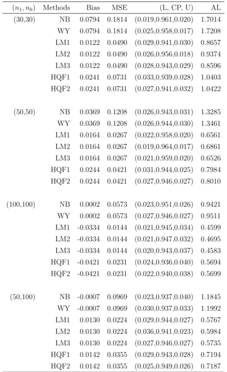
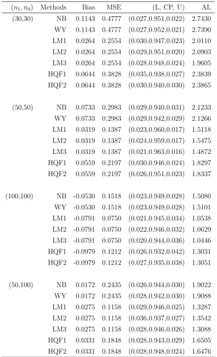
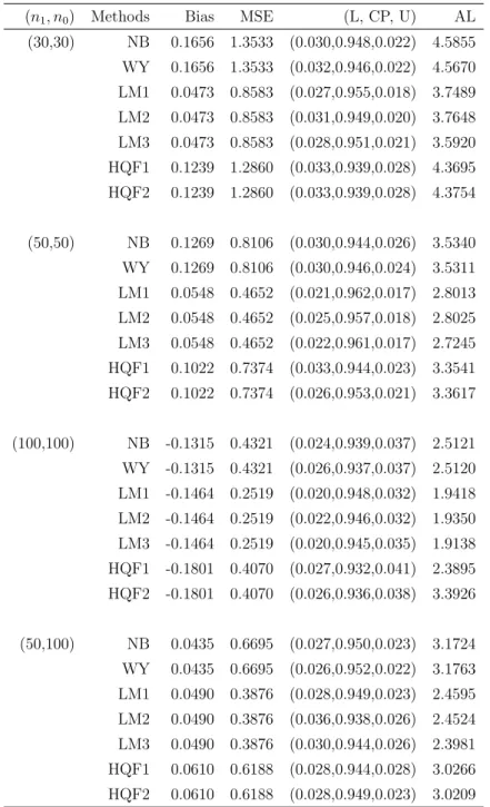
Simulation results under Model (I) are reported in Tables 2.1-2.3. Here are some key observations: (1) All point estimators have negligible bias, with the imputation-based estimator ˆθlin
EL having the smallest MSE; (2) The estimator ˆθ
lin
EL outperforms ˆθHQF in all
cases, with the largest gain of efficiency under strong correlation between Y and Z (i.e., ρ = 0.8); (3) Both ˆθlinEL and ˆθHQF perform significantly better than NB and WY for all
scenarios considered; (4) All confidence intervals have coverage probabilities very close to the nominal value, including the different versions of LM and HQF and the naive method NB and the EL method WY; (5) The three versions of LM confidence intervals are much shorter than other intervals; (6) All confidence intervals have balanced tail error rates under the simulation settings.
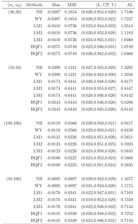
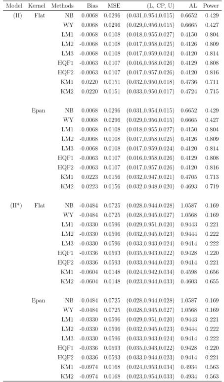
Results under Model (II) are summarized in Tables 2.4-2.6. Note that the model has two baseline variables and an intercept. The most striking observation is that both the LM approach and the HQF method perform well but the difference between the two disappears. This is consistent with the results of the theoretical comparisons discussed in Section 2.5. The second part of the simulation studies examines the effect of model misspecifications.
We include the kernel regression-based method presented in Section 2.4 as part of the comparisons. We consider two kernel functions: the flat kernel function K(u) = 1/2,
|u| ≤ 1, denoted as “Flat”, and the Epanechnikov kernel function K(u) = 3/4(1−u2),
|u| ≤ 1, denoted as “Epan”, for the case of univariate Z. For the case of two baseline variables, we use K(u1, u2) = K(u1)∗K(u2). The bandwidth hn for each simulation is
chosen by a 10-fold cross validation. In addition to the two linear models (I) and (II), we also consider two nonlinear models. Model (I*) involves a single Z variable:
Y1i = θ0+ 4 sin(Z1i) +ε1i, i= 1,· · · , n1,
Y0j = 4 sin(Z0j) +ε0j, j = 1,· · · , n0.
Model (II*) involves two baseline variables X and Z:
Y1i = θ0+ 4 sin(X1i+Z1i) +ε1i, i= 1,· · · , n1,
Y0j = 4 sin(X0j +Z0j) +ε0j, j = 1,· · · , n0.
The baseline variables are generated in the same way as in the two linear models. The error terms ε1i and ε0j are generated fromN(0,22). The parameter θ0 is the true value of
the treatment effect E(Y1)−E(Y0). We consider larger sample sizes n1 =n0 = 200 in this
case, due to the need for kernel smoothing. The truncation sequencebnis chosen as 0.0001
for Model (I*) and 0.05 for Model (II*). The point estimator under kernel regression is given by ˆθELker. Two confidence intervals on θ0 are constructed. The EL ratio confidence
interval based on Theorem 2 is denoted as KM1; the interval using the asymptotic variance and normal approximation is denoted as KM2.
The simulation results are reported in Table 2.7 for Models (I) and (I*) and in Table 2.8 for Models (II) and (II*). The value ofρis 0.80 for both Models (I) and (II). The true value of θ0 is set at 0.3. The last column of the two tables is the power for testing H0 :θ0 = 0.
The kernel regression method KM produces acceptable results under Models (I) and (II) but is less efficient than the LM method: bigger MSE, wider confidence intervals, and smaller power of the test. The kernel regression method, however, performs much better
under the two nonlinear models (I*) and (II*). The LM method fails completely under the Model (I*).
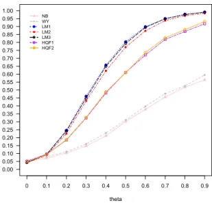
The last part of the simulation focuses on power functions, π(θ), of testing H0 :θ = 0
against H1 :θ 6= 0. The results are summarized by plots of the power functions presented
in Figures 2.1-2.4. Those plots reinforce what we have observed from the tables. Under Models (I) and (II), the three tests based on linear regression imputation are more powerful than all other tests. Under the two nonlinear Models (I*) and (II*), the two tests based on kernel regression imputation have much larger power. The comparisons are meaningful since all tests have similar size close to the nominal level 5%.
Table 2.1: Inferences on θ under Model (I), ρ= 0.8,θ0 = 0.3
(n1, n0) Methods Bias MSE (L, CP, U) AL
(30,30) NB 0.0794 0.1814 (0.019,0.961,0.020) 1.7014 WY 0.0794 0.1814 (0.025,0.958,0.017) 1.7208 LM1 0.0122 0.0490 (0.029,0.941,0.030) 0.8657 LM2 0.0122 0.0490 (0.026,0.956,0.018) 0.9374 LM3 0.0122 0.0490 (0.028,0.943,0.029) 0.8596 HQF1 0.0241 0.0731 (0.033,0.939,0.028) 1.0403 HQF2 0.0241 0.0731 (0.027,0.941,0.032) 1.0422 (50,50) NB 0.0369 0.1208 (0.026,0.943,0.031) 1.3285 WY 0.0369 0.1208 (0.026,0.944,0.030) 1.3461 LM1 0.0164 0.0267 (0.022,0.958,0.020) 0.6561 LM2 0.0164 0.0267 (0.019,0.964,0.017) 0.6861 LM3 0.0164 0.0267 (0.021,0.959,0.020) 0.6526 HQF1 0.0244 0.0421 (0.031,0.944,0.025) 0.7984 HQF2 0.0244 0.0421 (0.027,0.946,0.027) 0.8010 (100,100) NB 0.0002 0.0573 (0.023,0.951,0.026) 0.9421 WY 0.0002 0.0573 (0.027,0.946,0.027) 0.9511 LM1 -0.0334 0.0144 (0.021,0.945,0.034) 0.4599 LM2 -0.0334 0.0144 (0.021,0.947,0.032) 0.4695 LM3 -0.0334 0.0144 (0.020,0.943,0.037) 0.4583 HQF1 -0.0421 0.0231 (0.024,0.936,0.040) 0.5694 HQF2 -0.0421 0.0231 (0.022,0.940,0.038) 0.5699 (50,100) NB -0.0007 0.0969 (0.023,0.937,0.040) 1.1845 WY -0.0007 0.0969 (0.030,0.937,0.033) 1.1992 LM1 0.0130 0.0224 (0.029,0.944,0.027) 0.5767 LM2 0.0130 0.0224 (0.036,0.941,0.023) 0.5984 LM3 0.0130 0.0224 (0.027,0.946,0.027) 0.5735 HQF1 0.0142 0.0355 (0.029,0.943,0.028) 0.7194 HQF2 0.0142 0.0355 (0.025,0.949,0.026) 0.7187
Table 2.2: Inferences on θ under Model (I), ρ= 0.5,θ0 = 0.3
(n1, n0) Methods Bias MSE (L, CP, U) AL
(30,30) NB 0.1143 0.4777 (0.027,0.951,0.022) 2.7430 WY 0.1143 0.4777 (0.027,0.952,0.021) 2.7390 LM1 0.0264 0.2554 (0.030,0.947,0.023) 2.0110 LM2 0.0264 0.2554 (0.029,0.951,0.020) 2.0903 LM3 0.0264 0.2554 (0.028,0.948,0.024) 1.9605 HQF1 0.0644 0.3828 (0.035,0.938,0.027) 2.3839 HQF2 0.0644 0.3828 (0.030,0.940,0.030) 2.3865 (50,50) NB 0.0733 0.2983 (0.029,0.940,0.031) 2.1233 WY 0.0733 0.2983 (0.029,0.942,0.029) 2.1266 LM1 0.0319 0.1387 (0.023,0.960,0.017) 1.5118 LM2 0.0319 0.1387 (0.024,0.959,0.017) 1.5475 LM3 0.0319 0.1387 (0.021,0.963,0.016) 1.4872 HQF1 0.0559 0.2197 (0.030,0.946,0.024) 1.8297 HQF2 0.0559 0.2197 (0.026,0.951,0.023) 1.8337 (100,100) NB -0.0530 0.1518 (0.023,0.949,0.028) 1.5080 WY -0.0530 0.1518 (0.023,0.949,0.028) 1.5101 LM1 -0.0791 0.0750 (0.021,0.945,0.034) 1.0538 LM2 -0.0791 0.0750 (0.022,0.946,0.032) 1.0629 LM3 -0.0791 0.0750 (0.020,0.944,0.036) 1.0446 HQF1 -0.0979 0.1212 (0.026,0.932,0.042) 1.3031 HQF2 -0.0979 0.1212 (0.027,0.935,0.038) 1.3051 (50,100) NB 0.0172 0.2435 (0.026,0.944,0.030) 1.9022 WY 0.0172 0.2435 (0.028,0.942,0.030) 1.9088 LM1 0.0275 0.1158 (0.029,0.946,0.025) 1.3287 LM2 0.0275 0.1158 (0.036,0.937,0.027) 1.3542 LM3 0.0275 0.1158 (0.028,0.946,0.026) 1.3088 HQF1 0.0331 0.1848 (0.028,0.943,0.029) 1.6505 HQF2 0.0331 0.1848 (0.028,0.948,0.024) 1.6476
Table 2.3: Inferences on θ under Model (I), ρ= 0.3,θ0 = 0.3
(n1, n0) Methods Bias MSE (L, CP, U) AL
(30,30) NB 0.1656 1.3533 (0.030,0.948,0.022) 4.5855 WY 0.1656 1.3533 (0.032,0.946,0.022) 4.5670 LM1 0.0473 0.8583 (0.027,0.955,0.018) 3.7489 LM2 0.0473 0.8583 (0.031,0.949,0.020) 3.7648 LM3 0.0473 0.8583 (0.028,0.951,0.021) 3.5920 HQF1 0.1239 1.2860 (0.033,0.939,0.028) 4.3695 HQF2 0.1239 1.2860 (0.033,0.939,0.028) 4.3754 (50,50) NB 0.1269 0.8106 (0.030,0.944,0.026) 3.5340 WY 0.1269 0.8106 (0.030,0.946,0.024) 3.5311 LM1 0.0548 0.4652 (0.021,0.962,0.017) 2.8013 LM2 0.0548 0.4652 (0.025,0.957,0.018) 2.8025 LM3 0.0548 0.4652 (0.022,0.961,0.017) 2.7245 HQF1 0.1022 0.7374 (0.033,0.944,0.023) 3.3541 HQF2 0.1022 0.7374 (0.026,0.953,0.021) 3.3617 (100,100) NB -0.1315 0.4321 (0.024,0.939,0.037) 2.5121 WY -0.1315 0.4321 (0.026,0.937,0.037) 2.5120 LM1 -0.1464 0.2519 (0.020,0.948,0.032) 1.9418 LM2 -0.1464 0.2519 (0.022,0.946,0.032) 1.9350 LM3 -0.1464 0.2519 (0.020,0.945,0.035) 1.9138 HQF1 -0.1801 0.4070 (0.027,0.932,0.041) 2.3895 HQF2 -0.1801 0.4070 (0.026,0.936,0.038) 3.3926 (50,100) NB 0.0435 0.6695 (0.027,0.950,0.023) 3.1724 WY 0.0435 0.6695 (0.026,0.952,0.022) 3.1763 LM1 0.0490 0.3876 (0.028,0.949,0.023) 2.4595 LM2 0.0490 0.3876 (0.036,0.938,0.026) 2.4524 LM3 0.0490 0.3876 (0.030,0.944,0.026) 2.3981 HQF1 0.0610 0.6188 (0.028,0.944,0.028) 3.0266 HQF2 0.0610 0.6188 (0.028,0.949,0.023) 3.0209
Table 2.4: Inferences onθ under Model (II), ρ= 0.8, θ0 = 0.3
(n1, n0) Methods Bias MSE (L, CP, U) AL
(30,30) NB -0.0387 0.1854 (0.026,0.954,0.020) 1.7186 WY -0.0387 0.1854 (0.026,0.952,0.022) 1.7227 LM1 -0.0410 0.0736 (0.023,0.944,0.033) 1.0514 LM2 -0.0410 0.0736 (0.020,0.952,0.028) 1.1183 LM3 -0.0410 0.0736 (0.024,0.945,0.031) 1.0460 HQF1 -0.0275 0.0749 (0.023,0.946,0.031) 1.0749 HQF2 -0.0275 0.0749 (0.026,0.942,0.032) 1.0460 (50,50) NB 0.0399 0.1221 (0.027,0.945,0.028) 1.3295 WY 0.0399 0.1221 (0.028,0.942,0.030) 1.3356 LM1 0.0174 0.0441 (0.026,0.948,0.026) 0.8177 LM2 0.0174 0.0441 (0.018,0.955,0.027) 0.8447 LM3 0.0174 0.0441 (0.028,0.946,0.026) 0.8142 HQF1 0.0243 0.0443 (0.028,0.946,0.026) 0.8286 HQF2 0.0243 0.0443 (0.029,0.945,0.026) 0.8142 (100,100) NB -0.0119 0.0566 (0.029,0.950,0.021) 0.9417 WY -0.0119 0.0566 (0.029,0.950,0.021) 0.9450 LM1 -0.0123 0.0226 (0.023,0.951,0.026) 0.5851 LM2 -0.0123 0.0226 (0.024,0.951,0.025) 0.5923 LM3 -0.0123 0.0226 (0.024,0.950,0.026) 0.5835 HQF1 -0.0100 0.0225 (0.024,0.952,0.024) 0.5868 HQF2 -0.0100 0.0225 (0.025,0.951,0.024) 0.5835 (50,100) NB -0.0005 0.0897 (0.029,0.942,0.029) 1.1677 WY -0.0005 0.0897 (0.031,0.943,0.026) 1.1715 LM1 -0.0176 0.0341 (0.022,0.947,0.031) 0.7163 LM2 -0.0176 0.0341 (0.019,0.952,0.029) 0.7359 LM3 -0.0176 0.0341 (0.022,0.946,0.032) 0.7134 HQF1 -0.0145 0.0339 (0.020,0.948,0.032) 0.7252 HQF2 -0.0145 0.0339 (0.023,0.946,0.031) 0.7134
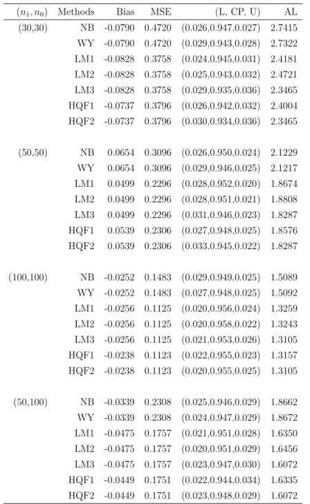
Table 2.5: Inferences onθ under Model (II), ρ= 0.5, θ0 = 0.3
(n1, n0) Methods Bias MSE (L, CP, U) AL
(30,30) NB -0.0790 0.4720 (0.026,0.947,0.027) 2.7415 WY -0.0790 0.4720 (0.029,0.943,0.028) 2.7322 LM1 -0.0828 0.3758 (0.024,0.945,0.031) 2.4181 LM2 -0.0828 0.3758 (0.025,0.943,0.032) 2.4721 LM3 -0.0828 0.3758 (0.029,0.935,0.036) 2.3465 HQF1 -0.0737 0.3796 (0.026,0.942,0.032) 2.4004 HQF2 -0.0737 0.3796 (0.030,0.934,0.036) 2.3465 (50,50) NB 0.0654 0.3096 (0.026,0.950,0.024) 2.1229 WY 0.0654 0.3096 (0.029,0.946,0.025) 2.1217 LM1 0.0499 0.2296 (0.028,0.952,0.020) 1.8674 LM2 0.0499 0.2296 (0.028,0.951,0.021) 1.8808 LM3 0.0499 0.2296 (0.031,0.946,0.023) 1.8287 HQF1 0.0539 0.2306 (0.027,0.948,0.025) 1.8576 HQF2 0.0539 0.2306 (0.033,0.945,0.022) 1.8287 (100,100) NB -0.0252 0.1483 (0.029,0.949,0.025) 1.5089 WY -0.0252 0.1483 (0.027,0.948,0.025) 1.5092 LM1 -0.0256 0.1125 (0.020,0.956,0.024) 1.3259 LM2 -0.0256 0.1125 (0.020,0.958,0.022) 1.3243 LM3 -0.0256 0.1125 (0.021,0.953,0.026) 1.3105 HQF1 -0.0238 0.1123 (0.022,0.955,0.023) 1.3157 HQF2 -0.0238 0.1123 (0.020,0.955,0.025) 1.3105 (50,100) NB -0.0339 0.2308 (0.025,0.946,0.029) 1.8662 WY -0.0339 0.2308 (0.024,0.947,0.029) 1.8672 LM1 -0.0475 0.1757 (0.021,0.951,0.028) 1.6350 LM2 -0.0475 0.1757 (0.020,0.951,0.029) 1.6456 LM3 -0.0475 0.1757 (0.023,0.947,0.030) 1.6072 HQF1 -0.0449 0.1751 (0.022,0.944,0.034) 1.6335 HQF2 -0.0449 0.1751 (0.023,0.948,0.029) 1.6072
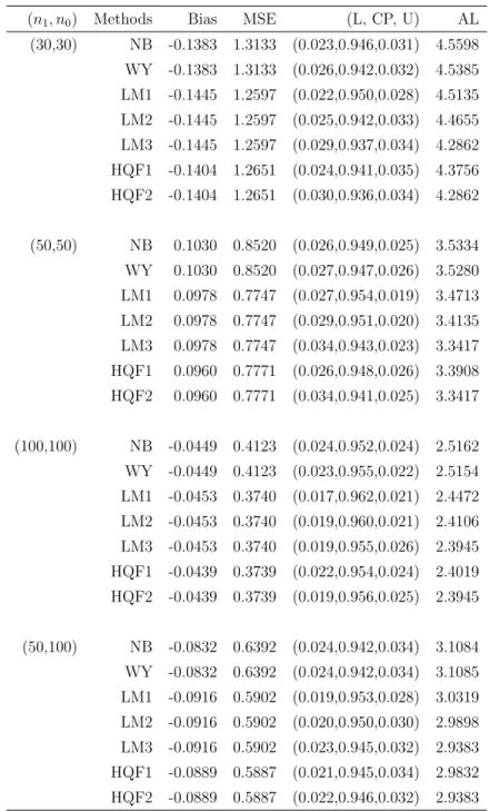
Table 2.6: Inferences onθ under Model (II), ρ= 0.3, θ0 = 0.3
(n1, n0) Methods Bias MSE (L, CP, U) AL
(30,30) NB -0.1383 1.3133 (0.023,0.946,0.031) 4.5598 WY -0.1383 1.3133 (0.026,0.942,0.032) 4.5385 LM1 -0.1445 1.2597 (0.022,0.950,0.028) 4.5135 LM2 -0.1445 1.2597 (0.025,0.942,0.033) 4.4655 LM3 -0.1445 1.2597 (0.029,0.937,0.034) 4.2862 HQF1 -0.1404 1.2651 (0.024,0.941,0.035) 4.3756 HQF2 -0.1404 1.2651 (0.030,0.936,0.034) 4.2862 (50,50) NB 0.1030 0.8520 (0.026,0.949,0.025) 3.5334 WY 0.1030 0.8520 (0.027,0.947,0.026) 3.5280 LM1 0.0978 0.7747 (0.027,0.954,0.019) 3.4713 LM2 0.0978 0.7747 (0.029,0.951,0.020) 3.4135 LM3 0.0978 0.7747 (0.034,0.943,0.023) 3.3417 HQF1 0.0960 0.7771 (0.026,0.948,0.026) 3.3908 HQF2 0.0960 0.7771 (0.034,0.941,0.025) 3.3417 (100,100) NB -0.0449 0.4123 (0.024,0.952,0.024) 2.5162 WY -0.0449 0.4123 (0.023,0.955,0.022) 2.5154 LM1 -0.0453 0.3740 (0.017,0.962,0.021) 2.4472 LM2 -0.0453 0.3740 (0.019,0.960,0.021) 2.4106 LM3 -0.0453 0.3740 (0.019,0.955,0.026) 2.3945 HQF1 -0.0439 0.3739 (0.022,0.954,0.024) 2.4019 HQF2 -0.0439 0.3739 (0.019,0.956,0.025) 2.3945 (50,100) NB -0.0832 0.6392 (0.024,0.942,0.034) 3.1084 WY -0.0832 0.6392 (0.024,0.942,0.034) 3.1085 LM1 -0.0916 0.5902 (0.019,0.953,0.028) 3.0319 LM2 -0.0916 0.5902 (0.020,0.950,0.030) 2.9898 LM3 -0.0916 0.5902 (0.023,0.945,0.032) 2.9383 HQF1 -0.0889 0.5887 (0.021,0.945,0.034) 2.9832 HQF2 -0.0889 0.5887 (0.022,0.946,0.032) 2.9383
Table 2.7: Comparisons with Model Misspecifications: (I) and (I*)
Model Kernel Methods Bias MSE (L, CP, U) AL Power
(I) Flat NB -0.0010 0.0312 (0.030,0.940,0.030) 0.6648 0.432 WY -0.0010 0.0312 (0.032,0.940,0.028) 0.6684 0.436 LM1 0.0096 0.0064 (0.021,0.958,0.021) 0.3262 0.953 LM2 0.0096 0.0064 (0.018,0.961,0.021) 0.3234 0.956 LM3 0.0096 0.0064 (0.017,0.958,0.025) 0.3228 0.955 HQF1 0.0122 0.0101 (0.022,0.955,0.023) 0.4026 0.828 HQF2 0.0122 0.0101 (0.020,0.958,0.022) 0.4033 0.831 KM1 -0.0126 0.0124 (0.029,0.948,0.023) 0.4239 0.780 KM2 -0.0126 0.0124 (0.028,0.945,0.027) 0.4217 0.776 Epan NB -0.0010 0.0312 (0.030,0.940,0.030) 0.6648 0.432 WY -0.0010 0.0312 (0.032,0.940,0.028) 0.6684 0.436 LM1 0.0096 0.0064 (0.021,0.958,0.021) 0.3262 0.953 LM2 0.0096 0.0064 (0.018,0.961,0.021) 0.3234 0.956 LM3 0.0096 0.0064 (0.017,0.958,0.025) 0.3228 0.955 HQF1 0.0122 0.0101 (0.022,0.955,0.023) 0.4026 0.828 HQF2 0.0122 0.0101 (0.020,0.958,0.022) 0.4033 0.831 KM1 -0.0096 0.0120 (0.029,0.947,0.024) 0.4170 0.794 KM2 -0.0096 0.0120 (0.027,0.948,0.025) 0.4152 0.788 (I*) Flat NB 0.0111 0.0743 (0.026,0.956,0.018) 1.1015 0.182 WY 0.0111 0.0743 (0.026,0.957,0.017) 1.0987 0.184 LM1 -0.5028 0.0278 (0.000,0.458,0.542) 0.2841 0.546 LM2 -0.5028 0.0278 (0.000,0.446,0.554) 0.2812 0.554 LM3 -0.5028 0.0278 (0.000,0.447,0.553) 0.2815 0.553 HQF1 -0.0080 0.0198 (0.024,0.944,0.032) 0.5567 0.549 HQF2 -0.0080 0.0198 (0.025,0.945,0.030) 0.5554 0.566 KM1 -0.0040 0.0102 (0.028,0.949,0.023) 0.3907 0.840 KM2 -0.0040 0.0102 (0.028,0.949,0.023) 0.3912 0.839 Epan NB 0.0111 0.0743 (0.026,0.956,0.018) 1.1015 0.182 WY 0.0111 0.0743 (0.026,0.957,0.017) 1.0987 0.184 LM1 -0.5028 0.0278 (0.000,0.458,0.542) 0.2841 0.546 LM2 -0.5028 0.0278 (0.000,0.446,0.554) 0.2812 0.554 LM3 -0.5028 0.0278 (0.000,0.447,0.553) 0.2815 0.553 HQF1 -0.0080 0.0198 (0.024,0.944,0.032) 0.5567 0.549 HQF2 -0.0080 0.0198 (0.025,0.945,0.030) 0.5554 0.566 KM1 -0.0028 0.0101 (0.027,0.950,0.023) 0.3876 0.841 KM2 -0.0028 0.0101 (0.027,0.950,0.023) 0.3881 0.840
Table 2.8: Comparisons with Model Misspecifications: (II) and (II*)
Model Kernel Methods Bias MSE (L, CP, U) AL Power
(II) Flat NB 0.0068 0.0296 (0.031,0.954,0.015) 0.6652 0.429 WY 0.0068 0.0296 (0.029,0.956,0.015) 0.6665 0.427 LM1 -0.0068 0.0108 (0.018,0.955,0.027) 0.4150 0.804 LM2 -0.0068 0.0108 (0.017,0.958,0.025) 0.4126 0.809 LM3 -0.0068 0.0108 (0.017,0.959,0.024) 0.4120 0.814 HQF1 -0.0063 0.0107 (0.016,0.958,0.026) 0.4129 0.808 HQF2 -0.0063 0.0107 (0.017,0.957,0.026) 0.4120 0.816 KM1 0.0220 0.0151 (0.032,0.950,0.018) 0.4736 0.711 KM2 0.0220 0.0151 (0.033,0.950,0.017) 0.4724 0.715 Epan NB 0.0068 0.0296 (0.031,0.954,0.015) 0.6652 0.429 WY 0.0068 0.0296 (0.029,0.956,0.015) 0.6665 0.427 LM1 -0.0068 0.0108 (0.018,0.955,0.027) 0.4150 0.804 LM2 -0.0068 0.0108 (0.017,0.958,0.025) 0.4126 0.809 LM3 -0.0068 0.0108 (0.017,0.959,0.024) 0.4120 0.814 HQF1 -0.0063 0.0107 (0.016,0.958,0.026) 0.4129 0.808 HQF2 -0.0063 0.0107 (0.017,0.957,0.026) 0.4120 0.816 KM1 0.0223 0.0156 (0.032,0.947,0.021) 0.4705 0.713 KM2 0.0223 0.0156 (0.032,0.948,0.020) 0.4693 0.719 (II*) Flat NB -0.0484 0.0725 (0.028,0.944,0.028) 1.0