Predicting Head Pose from Speech with a
Conditional Variational Autoencoder
David Greenwood, Stephen Laycock, Iain Matthews
School of Computing Sciences
University of East Anglia
United Kingdom
[email protected], [email protected], [email protected]
Abstract
Natural movement plays a significant role in realistic speech an-imation. Numerous studies have demonstrated the contribution visual cues make to the degree we, as human observers, find an animation acceptable.
Rigid head motion is one visual mode that universally co-occurs with speech, and so it is a reasonable strategy to seek a transformation from the speech mode to predict the head pose. Several previous authors have shown that prediction is possi-ble, but experiments are typically confined to rigidly produced dialogue. Natural, expressive, emotive and prosodic speech ex-hibit motion patterns that are far more difficult to predict with considerable variation in expected head pose.
Recently, Long Short Term Memory (LSTM) networks have become an important tool for modelling speech and nat-ural language tasks. We employ Deep Bi-Directional LSTMs (BLSTM) capable of learning long-term structure in language, to model the relationship that speech has with rigid head tion. We then extend our model by conditioning with prior mo-tion. Finally, we introduce a generative head motion model, conditioned on audio features using a Conditional Variational Autoencoder (CVAE). Each approach mitigates the problems of the one to many mapping that a speech to head pose model must accommodate.
Index Terms: speech animation, head motion synthesis, visual prosody, generative models, BLSTM, CVAE
1. Introduction
Speech animation involves transforming and deforming a char-acter model, temporally synchronised to an audible utterance to give the appearance that the model is speaking. Given the close relationship between speech and gesture, the problem is challenging, as human viewers are very sensitive to natural hu-man movement. Practical applications of speech animation, for example computer games and animated films, often rely on mo-tion capture devices or hand keyed animamo-tion. Demand for re-alistic animation within these domains is high and both of these approaches are expensive and time consuming, providing con-siderable motivation for automation of the process.
Human discourse essentially flows in two modes: the ex-plicit mode of audible speech that carries the semantic meaning of some utterance, and a more supportive visual mode where non-verbal gestures complement and enhance the audible mode. Research suggests that speech and gesture stem from the same internal process and share the same semantic meaning [1, 2].
Speaker head motion is a rather interesting aspect of visual speech. Head motion has been shown to contribute to speech
comprehension [3], yet unlike the articulators, it is under inde-pendent control. As the audio channel contains the most com-plete information stream in an utterance, it is a reasonable strat-egy to seek a mapping from within this stream that might enable plausible predictions of head pose. Indeed, there is significant measurable correlation between speech and head motion [4, 5]. When we speak, we encapsulate the semantics of our utter-ance in the words of our language. We have already stated that rigid head motion is strongly tied to speech, but consider how that occurs. For example, if we are expressing agreement, nod-ding the head is a common gestural supplement. However, just considering that simple gesture, speaking the same utterance at another time could well have the nodding action at a different phase or frequency. In considering just that simple case, we can appreciate that head pose should be considered as a one to many mapping. And yet there is more to it. When we speak naturally, we do not issue a monotone dialogue, our voices are highly
an-imated. We use expression, emphasis, intonation orprosodyto
make speech much more than merely words. With that in mind, we must now consider that speech to head motion has a very diverse expectation.
There have been a number of researchers interested in pre-dicting head motion from speech in recent years. Initial stud-ies took the approach of clustering head motion patterns and giving class labels [6, 7, 5]. Hidden Markov Models (HMMs) were trained for each cluster, modelling the relation between the speech features and head motion. Hofer [4, 8] observes the limitations of the frame wise approach of his predecessors, and proposes a trajectory based model. More recently Ben-Youssef [9] proposed an improved clustering for motion. All of these approaches rely on a suitable labelling of motion units, either manually or automatically, which is a challenging problem in itself.
Recently, the Graphics Processor Unit (GPU) has enabled efficient training of Deep Neural Networks (DNNs), and within many aspects of speech and language processing, DNNs are now state of the art [10, 11, 12]. DNNs were proposed as a
modelling strategy for head motion prediction by Ding et al.
[13]. Using a deep Feed-Forward Neural Network (FFN) re-gression model to predict Euler angles of nod, yaw and roll, they were able to report advantages over the previous HMM based approaches and were able to avoid the problem of clus-tering motion. Although deep FFNs are a powerful modelling tool, capable of learning complex non-linear mappings, they are limited in their ability to model long term temporal data.
The Long Short Term Memory (LSTM), introduced by Hochreiter [14] and further investigated by Gers [15], has been used to great effect in many domains arguably related to the speech to head pose problem. Graves [16], demonstrated the
ability of LSTM networks to model long term structure by pre-dicting discrete text values, and by prepre-dicting the real values
of hand-writing trajectories. Another example by Sutskeveret
al. [17] reports state of the art performance for the language
translation task. Ding et al. [18] introduced Bi-Directional
Long Short Term Memory (BLSTM) networks to the head mo-tion task, noting improvements over their own earlier work [13]. More recently Haag [19] uses BLSTMs and Bottleneck features [20] and noted a subtle improvement.
In the past few years, generative models [21, 22], train-able with back propagation [23] have taken an important step in learning, with models that can perform probabilistic inference
and make diverse predictions. Bowmanet al. [24] employed
a Variational Autoencoder (VAE) for natural language
gener-ation. Walker et al. [25] used a Conditional Variational
Au-toencoder (CVAE) to predict video motion vectors conditioned by a single image. To our knowledge, generative models have not yet been used for head motion prediction so we introduce a CVAE to the head motion synthesis task here.
2. Corpus
Recent head motion prediction studies use data that is not widely available. In fact there are few significant corpora freely available that are suitable for modelling any rigid gesture with speech. For our own research we collected data as described in this section.
2.1. Data Collection
We invited two actors, one female (speaker A), one male (speaker B) to recite from a scripted set of short conversa-tional scenarios. The actors were encouraged to speak emo-tively and emphatically in order to provide natural, expressive and prosodic speech. In all, 3600 utterances were captured, giv-ing a total of around six hours of speech.
We used six cameras to record with synchronised frame timing, with three cameras aimed at each actor. Recording frequency was 59.94 Frames per Second (FPS) and resolution
1280×720pixels (720p). Audio was recorded simultaneously
at 48 kHz and later down sampled to 16 kHz.
Each actor had 62 landmarks distributed about the face, which along with 58 natural feature landmarks such as eyes and lip edges, were tracked with Active Appearance Models (AAMs) [26]. With the cameras arranged such that left and right stereo pairs were formed on each actor, we were able to derive 3D models. The 3D models were stabilised by selecting the least deformed points and, using Procrustes analysis [27], rigid motion was separated from deformation. The rotations are about the X,Y and Z axes of a right handed coordinate system, with Y pointing up.
2.2. Feature Extraction
We used a sliding frame over the time domain audio signal of
2/59.94swith an overlap of1/59.94s, matching the sampling
rate of our motion data. Following convention, each frame was multiplied by a Hamming window. Although we have experi-mented with many audio features, for this report we use the log
of the filter bank values as described by Denget al.in [11].
Un-der this scenario we have a feature vector of 40 audio samples temporally aligned with the 3 Euler angles: nod (x), yaw (y) and roll (z). We normalise all our data to have unit variance and zero mean.
3. Model Topology
All of our modelling strategies feature LSTM networks, al-though there are many variations to consider, we describe the
LSTM,H, in the equations (1) - (6): it=σ(Wixt+Uiht−1+bi) (1) ˜ Ct=tanh(Wcxt+Ucht−1+bc) (2) ft=σ(Wfxt+Ufht−1+bf) (3) Ct=it∗C˜t+ft∗Ct−1 (4) ot=σ(Woxt+Uoht−1+bo) (5) ht=ot∗tanh(Ct) (6)
whereσis a sigmoid function andi, o, f, Care the input
gate, output gate, forget gate and memory cell respectively.
3.1. Bi-Directional Long Short Term Memory (BLSTM)
Our application of the BLSTM differs from Dinget al. [18].
Instead of predicting one motion coefficient at each time step,
we predict a short span:1≤k ≤29. This allows observation
of frame-wise variation in prediction and permits options on re-combining each frame. For this report we simply take the mean at each predicted time step. Notably, we do not apply any post process to the prediction. We observed distinct motion events in
our data>500msand to ensure capturing these events the
re-ceptive field was29≤n≤129time steps,n/59.94s. Figure
1 illustrates the topology of our deep BLSTM showing that for each time step of audio features, we predict the corresponding time step of head motion.
t1 F t3 F tn F t2 F F F F F h1 F h3 F hn F h2 F
predicted motion output
speech features input
Figure 1:BLSTM network predicts one motion time step at each
speech time step.
3.2. BLSTM with Prior Motion Conditioning
Recall that we regard head motion as having many possible pre-dictions for an utterance. One approach to mitigate this situa-tion, that we present now, is to provide a prior motion hint to our model. Head motion is constrained by anatomy and kinematics. If we establish the dynamic state of head pose at the start of the event we wish to predict, we reduce the range of possible outcomes, particularly in the near term. The concept is
some-what related to the work by Chenet al. in [28], however their
work involves the use of recurrent decision trees to predict tele-vision camera motion at sporting events. We show the topology of this network in Figure 2. We accommodate the difference in time steps by emitting from the final state of our motion input BLSTM, and repeating to match the output duration.
x1 F xn F x2 F x1 F x3 F xn F x2 F F F F F F F F C C C C h1 F h3 F hn F h2 F
prior motion input audio features input predicted motion output
F C BLSTM concatenation vector input vector output
Figure 2:Adding a kinetic constraint with prior motion. During
prediction, the output is recursively fed to the motion input.
3.3. Conditional Variational Autoencoder (CVAE)
A Variational Autoencoder (VAE) comprises an encoder and a
decoder. The encoder,Qθ(z|x), seeks to represent input datax
in a latent spacezwith weights and biasesθ, where the encoder
outputs the parameters of a Gaussian probability density. The
decoder, Pφ(x|z), with weights and biasesφ, transforms the
parameters to the distribution of the original data. The CVAE adds a conditioning element to the VAE, such that the encoder
becomesQθ(z|x, c), and the decoder isPφ(x, c|z). Figure 3
shows the topology of our CVAE, using BLSTMs as the encoder and decoder. t1 t 2 t 3 t n BL ST M BL ST M BL ST M BL ST M t1 t 2 t 3 t n encoder decoder
head motion conditioning audio
Figure 3: By sampling from a Gaussian the CVAE model can
predict a range of expected motion.
4. Model Training
We trained the networks on our data, split 80% for training, 10% for validation and 10% for testing. Our objective function is Mean Squared Error (MSE), except for the CVAE model which has a custom objective function: the sum of the reconstruction loss and the Kullback-Leibler divergence [21]. Our
optimis-ing function isRMSprop[29], we set an initial learning rate of
10−3. Training continues until no further improvement on the
validation set, with a patience of 5 epochs. Model weights are saved at each epoch. We reload the best weights, decrement the
learning rate by a factor of 10 until10−5
, finally stopping at the best validation error. We then select the model with the low-est overall validation error. For this report, we present models trained on a single speaker, speaker A from our corpus. The total number of examples presented to the network at training
time depends somewhat on the value of spankand time steps
n, and is approximately7×104to3×105.
5. Results
To make comparison between each modelling scenario we plot some results from a highly expressive utterance made by speaker A. This example has not been part of the training or validation regime and is randomly selected:
“ I can’t breathe, because you smell like garbage juice, or rotten meat or something...”
Reconstruction simply involves presenting a test utterance and forward propagating through each network. Each resulting
motion coefficient has1tokvalues, of which we take the mean.
5.1. BLSTM
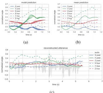
We examine the results from our first network variation in Fig-ure 4. FigFig-ure 4a shows the values directly returned from our model. Each frame-wise span is shown, and we can observe how coherently the model predicts each time step. We notice some variation at each step, and when we take the mean at each motion coefficient, the plot in Figure 4b shows some smoothing as a result. We rebuild the entire utterance in Figure 4c, which shows head motion over the audio waveform. We can observe that our prediction responds to the audio and matches a number of significant events in the ground truth. Note, we do not expect the prediction to closely match the ground truth, as the speech to head pose mapping is diverse. The ground truth however, does provide a good visual comparison to where we expect motion events to occur. 0.0 0.2 0.4 0.6 0.8 1.0 1.2 time (s) 0.1 0.0 0.1 0.2 0.3 0.4 0.5 0.6 0.7 normalised angle model prediction X pred Y pred Z pred X true Y true Z true (a) 0.0 0.2 0.4 0.6 0.8 1.0 1.2 time (s) 0.1 0.0 0.1 0.2 0.3 0.4 0.5 0.6 0.7 normalised angle mean prediction X pred Y pred Z pred X true Y true Z true (b) 0 1 2 3 4 5 6 7 time (s) 0.6 0.4 0.2 0.0 0.2 0.4 0.6 0.8 normalised angle reconstructed utterance audio X pred Y pred Z pred X true Y true Z true (c)
Figure 4: Predicted head motion from BLSTM, (a) is the
pre-diction directly from the model, showing frame-wise span, (b) shows the mean at each time step. Figure (c) shows reconstruc-tion of the example utterance. The result is plotted over the au-dio waveform to show the alignment of key events in the speech.
5.2. Motion Prior
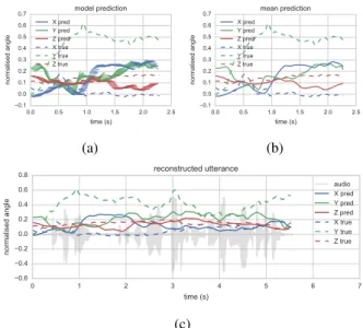
We show the reconstruction from our second model in Figure 5. Similarly, Figure 5a shows the direct output of our model, and Figure 5b shows the mean at each motion coefficient. This
example shows an extended duration,n= 129time steps. The model is provided with a motion hint of the first part of the ground truth of 45 time steps, leaving the remaining period un-seeded. Notice the model does not simply learn the identity for the seeded period. This model exhibits lower variance at each time step, and we find this is consistent throughout our exper-iments with this architecture. Figure 5c shows the reconstruc-tion of the entire utterance. We can rebuild an utterance from this model by recursively applying the prediction as the motion seed value. We observe that this model adheres more closely to the ground truth for the entire utterance. Although again, we do not expect exact matching, but when the prediction arrives at a value close to the ground truth the mapping space for future prediction is much smaller.
0.0 0.5 1.0 1.5 2.0 2.5 time (s) 0.1 0.0 0.1 0.2 0.3 0.4 0.5 0.6 0.7
normalised angle unseeded
model prediction X pred Y pred Z pred X true Y true Z true (a) 0.0 0.5 1.0 1.5 2.0 2.5 time (s) 0.1 0.0 0.1 0.2 0.3 0.4 0.5 0.6 0.7
normalised angle unseeded
mean prediction X pred Y pred Z pred X true Y true Z true (b) 0 1 2 3 4 5 6 7 time (s) 0.6 0.4 0.2 0.0 0.2 0.4 0.6 0.8 normalised angle reconstructed utterance audio X pred Y pred Z pred X true Y true Z true (c)
Figure 5: Prior motion model. Figure (a) shows model output
and (b) shows point-wise mean. The full utterance reconstruc-tion shows how the model is guided by the moreconstruc-tion seed.
5.3. CVAE
Figure 6 shows the reconstruction of our example utterance us-ing our CVAE generative model. We make predictions from this model by sampling from the unit Gaussian space and con-ditioning with our example audio features. A parameter for this model, not present in the earlier models, is the size of the latent
space. For this report we show a model withzin 3 dimensions,
which we found to have no disadvantage to larger space. When predicting from this model we see variance at each time step, shown in Figure 6a, resulting in smoothing in our reconstruc-tion process. When we reconstruct the entire utterance, shown in Figure 6c, we can observe the prediction responds very well to the audio, matching key prosodic events of this very expres-sive utterance. One very interesting feature of this model is the ability to generate variations of each prediction by taking further Gaussian samples, but retaining the conditioning audio features.
6. Discussion
A number of previous authors evaluate results with a correlation measure or some other point-wise comparison. We strongly reject this method for the following reasons: We do not
ex-0.0 0.5 1.0 1.5 2.0 2.5 time (s) 0.1 0.0 0.1 0.2 0.3 0.4 0.5 0.6 0.7 normalised angle model prediction X pred Y pred Z pred X true Y true Z true (a) 0.0 0.5 1.0 1.5 2.0 2.5 time (s) 0.1 0.0 0.1 0.2 0.3 0.4 0.5 0.6 0.7 normalised angle mean prediction X pred Y pred Z pred X true Y true Z true (b) 0 1 2 3 4 5 6 7 time (s) 0.6 0.4 0.2 0.0 0.2 0.4 0.6 0.8 normalised angle reconstructed utterance audio X pred Y pred Z pred X true Y true Z true (c)
Figure 6: CVAE model, (a) shows model output, (b) shows
point-wise mean. The full reconstruction in (c) shows how well this model aligns motion events with audio events. In addition, we can predict alternative motion from the same audio.
pect a prediction to closely match the ground truth, rather, each should be one example of many appropriate trajectories. Further, head motion is quasi-periodic; one could easily mea-sure quite high correlation without necessarily having appro-priate motion. Much of the research predicting head motion from speech has been data driven. Many of the previous au-thors mentioned in this paper have accumulated their own data, and without standard corpora and reliable empirical measure-ment, comparison with prior work is problematic. Some au-thors have offered subjective tests, yet the scale of the tests are often small and so statistically unreliable. The question of what represents appropriate or plausible head motion during speech is unclear. Subjectively, we have observed certain key events support viewer acceptance, but we have not yet been able to identify exactly why this is the case. We do know however, that it is important to have correct motion [3], and also that we can identify when it’s not correct [30]. Developing a measurement of correct head motion, or indeed more broadly gesture, is an open and difficult problem, and we are actively pursuing this goal.
Our most interesting results come from the CVAE model, that solves the one to many mapping problem. We can predict a number of plausible motion trajectories by choosing new
val-ues forz, but with the same audio features. Quicktime movie
files are provided in the supplementary material showing further examples from all our models.
7. Conclusions
In this paper we have presented our work on predicting head pose from audio. We describe our corpora, and present mod-elling strategies that offer diverse but plausible outcomes for audio input. The LSTM has been a powerful tool in speech and language modelling, and as the encoder-decoder in our CVAE has shown great utility. We feel that generative models offer great promise to this field and we continue working in this area.
8. References
[1] D. McNeill,Hand and mind: What gestures reveal about thought. University of Chicago Press, 1992.
[2] J. Cassell, D. McNeill, and K.-E. McCullough, “Speech-gesture mismatches: Evidence for one underlying representation of lin-guistic and nonlinlin-guistic information,”Pragmatics & cognition, vol. 7, no. 1, pp. 1–34, 1999.
[3] K. G. Munhall, J. A. Jones, D. E. Callan, T. Kuratate, and E. Vatikiotis-Bateson, “Visual prosody and speech intelligibility: head movement improves auditory speech perception.” Psycho-logical science : A journal of the American PsychoPsycho-logical Society / APS, vol. 15, no. 2, pp. 133–137, 2004.
[4] G. Hofer and H. Shimodaira, “Automatic head motion prediction from speech data,” inEighth Annual Conference of the Interna-tional Speech Communication Association, 2007.
[5] C. Busso, Z. Deng, M. Grimm, U. Neumann, and S. Narayanan, “Rigid head motion in expressive speech animation: Analysis and synthesis,”IEEE Transactions on Audio, Speech, and Language Processing, vol. 15, no. 3, pp. 1075–1086, 2007.
[6] Z. Deng, S. Narayanan, C. Busso, and U. Neumann, “Audio-based head motion synthesis for avatar-based telepresence systems,” in Proceedings of the 2004 ACM SIGMM workshop on Effective telepresence. ACM, 2004, pp. 24–30.
[7] C. Busso, Z. Deng, U. Neumann, and S. Narayanan, “Natural head motion synthesis driven by acoustic prosodic features,”Journal of Visualization and Computer Animation, vol. 16, no. 3-4, pp. 283– 290, 2005.
[8] G. Hofer, H. Shimodaira, and J. Yamagishi, “Speech driven head motion synthesis based on a trajectory model,” in ACM SIG-GRAPH 2007 posters. ACM, 2007, p. 86.
[9] A. Ben Youssef, H. Shimodaira, and D. A. Braude, “Articulatory features for speech-driven head motion synthesis,”Proceedings of Interspeech, Lyon, France, 2013.
[10] J.-T. Huang, J. Li, and Y. Gong, “An analysis of convolutional neural networks for speech recognition,” in2015 IEEE Interna-tional Conference on Acoustics, Speech and Signal Processing (ICASSP). IEEE, 2015, pp. 4989–4993.
[11] L. Deng, J. Li, J.-T. Huang, K. Yao, D. Yu, F. Seide, M. Seltzer, G. Zweig, X. He, J. Williamset al., “Recent advances in deep learning for speech research at Microsoft,” inAcoustics, Speech and Signal Processing (ICASSP), 2013 IEEE International Con-ference on. IEEE, 2013, pp. 8604–8608.
[12] L. Deng, G. Hinton, and B. Kingsbury, “New types of deep neural network learning for speech recognition and related applications: An overview,” in2013 IEEE International Conference on Acous-tics, Speech and Signal Processing. IEEE, 2013, pp. 8599–8603. [13] C. Ding, L. Xie, and P. Zhu, “Head motion synthesis from speech using deep neural networks,”Multimedia Tools and Applications, pp. 1–18, 2014.
[14] S. Hochreiter and J. Schmidhuber, “Long short-term memory,” Neural computation, vol. 9, no. 8, pp. 1735–1780, 1997. [15] F. Gers, “Long short-term memory in recurrent neural networks,”
Ph.D. dissertation, Universit¨at Hannover, 2001.
[16] A. Graves, “Generating sequences with recurrent neural net-works,” CoRR, vol. abs/1308.0850, 2013. [Online]. Available: http://arxiv.org/abs/1308.0850
[17] I. Sutskever, O. Vinyals, and Q. V. Le, “Sequence to sequence learning with neural networks,” inAdvances in neural information processing systems, 2014, pp. 3104–3112.
[18] C. Ding, P. Zhu, and L. Xie, “Blstm neural networks for speech driven head motion synthesis,” inSixteenth Annual Conference of the International Speech Communication Association, 2015. [19] K. Haag and H. Shimodaira, “Bidirectional lstm networks
em-ploying stacked bottleneck features for expressive speech-driven head motion synthesis,” inInternational Conference on Intelligent Virtual Agents. Springer, 2016, pp. 198–207.
[20] J. Gehring, Y. Miao, F. Metze, and A. Waibel, “Extracting deep bottleneck features using stacked auto-encoders,” inAcoustics, Speech and Signal Processing (ICASSP), 2013 IEEE Interna-tional Conference on. IEEE, 2013, pp. 3377–3381.
[21] D. P. Kingma, S. Mohamed, D. J. Rezende, and M. Welling, “Semi-supervised learning with deep generative models,” in Ad-vances in Neural Information Processing Systems, 2014, pp. 3581–3589.
[22] D. J. Rezende, S. Mohamed, and D. Wierstra, “Stochastic back-propagation and approximate inference in deep generative mod-els,” inProceedings of The 31st International Conference on Ma-chine Learning, 2014, pp. 1278–1286.
[23] Y. Bengio, E. Laufer, G. Alain, and J. Yosinski, “Deep generative stochastic networks trainable by backprop,” inProceedings of The 31st International Conference on Machine Learning, 2014, pp. 226–234.
[24] S. R. Bowman, L. Vilnis, O. Vinyals, A. M. Dai, R. Jozefowicz, and S. Bengio, “Generating sentences from a continuous space,” CoNLL 2016, p. 10, 2016.
[25] J. Walker, C. Doersch, A. Gupta, and M. Hebert, “An uncertain future: Forecasting from static images using variational autoen-coders,” inEuropean Conference on Computer Vision. Springer, 2016, pp. 835–851.
[26] I. Matthews and S. Baker, “Active appearance models revisited,” International Journal of Computer Vision, vol. 60, no. 2, pp. 135– 164, 2004.
[27] J. C. Gower, “Generalized procrustes analysis,”Psychometrika, vol. 40, no. 1, pp. 33–51, 1975.
[28] J. Chen, H. M. Le, P. Carr, Y. Yue, and J. J. Little, “Learning online smooth predictors for realtime camera planning using re-current decision trees,” inProceedings of the IEEE Conference on Computer Vision and Pattern Recognition, 2016, pp. 4688–4696. [29] T. Tieleman and G. Hinton, “Lecture 6.5-rmsprop: Divide the gra-dient by a running average of its recent magnitude,”COURSERA: Neural networks for machine learning, vol. 4, no. 2, 2012. [30] M. Mori, “The uncanny valley,”Energy, vol. 7, no. 4, pp. 33–35,