TR
OP
E
R
HC
RA
ES
E
R
PAI
D
I
INVESTIGATION OF KNN CLASSIFIER ON
POSTERIOR FEATURES TOWARDS
APPLICATION IN AUTOMATIC SPEECH
RECOGNITION
Afsaneh Asaei Hervé Bourlard Benjamin Picart
Idiap-RR-11-2010
JUNE 2010
Centre du Parc, Rue Marconi 19, P.O. Box 592, CH - 1920 Martigny
1
INVESTIGATION OF KNN CLASSIFIER ON POSTERIOR
FEATURES TOWARDS APPLICATION IN AUTOMATIC SPEECH
RECOGNITION
Afsaneh Asaei1,2, Hervé Bourlard1,2, Benjamin Picart1,3
1IDIAP Research Institute, Martigny, Switzerland
2Ecole Polytechnique Fédérale de Lausanne (EPFL), Switzerland 3Faculté Polytechnique de Mons, (FPMs), Belgium
[email protected], [email protected], [email protected]
Abstract
Class posterior distributions can be used to classify or as intermediate features, which can be further exploited in different classifiers (e.g., Gaussian Mixture Models, GMM) towards improving speech recognition performance. In this paper we examine the possibility to use kNN classifier to perform local phonetic classification of class posterior distribution extracted from acoustic vectors. In that framework, we also propose and evaluate a new kNN metric based on the relative angle between feature vectors to define the nearest neighbors. This idea is inspired by the orthogonality characteristic of the posterior features. To fully exploit this attribute, kNN is used in two main steps: (1) the distance is computed as the cosine function of the relative angle between the test vector and the training vector and (2) the nearest neighbors are defined as the samples within a specific relative angle to the test data and the test samples which do not have enough labels in such a hyper-cone are considered as uncertainties and left undecided. This approach is evaluated on TIMIT database and compared to other metrics already used in literature for measuring the similarity between posterior probabilities. Based on our experiments, the proposed approach yield 78.48% frame level accuracy while specifying 15.17% uncertainties in the feature space.
1. Introduction
Posterior probabilities are currently often used as powerful features to improve automatic speech recognition (ASR) systems. The interesting ideas behind posterior probabilities are that they could be provided by discriminant training while accommodating acoustic context. This idea was first used in the development of the successful hybrid HMM/ANN system which initiated extensive use of posteriors in speech recognition systems. In this approach, emission probabilities required in HMM system is provided by a posteriori probabilities computed by an Artificial Neural Network (ANN), and more specifically by MLP [1]. Hence, in HMM/ANN the posterior probabilities are used as local classifiers. This application of posteriors as local measures was later explored in several other speech recognition purposes such as word lattice rescoring [2], beam search pruning [3] and confidence measures estimation [4]. On the other hand, posterior probabilities could be used as acoustic features. This approach was proposed and implemented in the state-of-the-art Tandem speech recognition system where posterior probabilities are used as the most discriminant and informative features. We further explain this system in the next section which goes through the details of posterior features.
In both main applications of posterior probabilities, either as local classifiers or as features, the system efficacy strongly depends on the quality of the estimated posteriors and compatibility of the
2
models and similarity measures used. To boost the quality of the posteriors, another classifier is often used, as a hierarchy, after the initial MLP in order to capture more phonetic and contextual information of the speech signal; whereas for model compatibility, posteriors are gaussianized and decorrelated to form the Tandem features and fed into the standard HMM/GMM or in KL-HMM, their distribution is directly used in HMM model where the similarity measure is modified to Kullback-Leibler divergence for better realization of posterior characteristics [ 5].
In this paper we examine the possibility of using kNN classifier to perform local phonetic classification of class posterior distribution. Figure 1 presents our model for this investigation. The crucial function which affects the performance of this classifier is the distance metric. Therefore, we have explored the functions that are already referenced in previous studies (Euclidian distance, Bhattacharyya distance and Kullback-Leibler divergence) and we have proposed to use the cosine function as a distance metric to exploit the orthogonality characteristic of posterior feature space.
PLP Features
Figure 1. Phoneme Classification by kNN Classifier
This paper is organized as follows: Section 2 explains posterior features. Starting with the idea of state-of-the art Tandem speech recognition, we go through the details of characteristics which make posteriors powerful features for speech recognition. In Section 3 we give a brief overview of the Nearest Neighbor classifier and the reasons why we selected this classifier for our investigation. Later in the sub-section 3.1, we propose a new approach for classification of the posterior features based on a geometric look into the posterior space. In Section 4 our experiments setup and results are given and finally we conclude at Section 5.
The notation used in this paper will be the following:
• , , … , , … , , an acoustic observation sequence
• , , … , , … , , the set of training posterior feature vectors
• , , … , , … , , the set of test posterior feature vectors
where posterior feature vector is a phone/class posterior distribution, e. g.:
, , … , , … , , where T stands for the transpose
operation, is the number of phone classes or cardinality of the set of all possible classes
, , … , , … , .
When referring to the feature vectors: represent the element of the training feature vector whereas represents the element of the test vector.
2. Posterior features
Posterior features were initially motivated as a simple scheme to take the advantage of both HMM/ANN and HMM/GMM speech recognition frameworks [ 6]. These features are extracted by an MLP using spectral-based features such as MFCC or PLP as input. In this approach, each output unit of the MLP is associated with a particular phoneme of the set of possible classes and it is trained to generate a posteriori probabilities of the output classes conditioned on the input acoustic observation sequence ( ), i.e. . While allowing for discriminant training, such an approach also has the advantage of possibly accommodating acoustic context by providing several frames at the MLP input, thus estimating , where is the length of the context window (typically equal to 4). However, context up to 50 has also been successfully used [ 7].
These MLP-generated phoneme posterior probabilities could be fed (after some transformation) as input acoustic feature vector into the standard HMM recognizer. Tandem has been the most
MLP
Transformation ClassificationkNN
3
successful system which made this scheme possible [ 8]. In this approach, the MLP posterior probability estimates are roughly gaussianized by computing the logarithm of the MLP output (a static nonlinearity) and whitened by the Karhunen-Loeve transform (KLT) derived from the training data. Such gaussianized and whitened posterior probabilities form the feature vector for the subsequent HMM/GMM recognizer. Thus, the conventional features derived from short-term spectrum representing the spectral envelope of the signal are replaced by the transformed posteriors of acoustic events (in the original concept the events were context-independent phonemes).
Input to Tandem can be any data that are believed to provide a relevant evidence for the classification. In its simplest form, Tandem takes as an input a superframe of typical conventional speech features such as 9 frames of concatenated PLP static and dynamic features. Usually, Tandem inputs are concatenated outputs from other sub-band classifiers (TRAP [ 7] or HATS [ 9]). TRAP has been also reported to be efficient in combining different features and for alleviating irrelevant information [ 10] [ 11].
In several aspects, posterior features posses important advantages compared to spectrum-based acoustic features:
1. The purpose of feature extraction is mainly to reduce the dimensionality of the speech signal while preserving (or enhancing) the discriminant information of the data. In this process, the irrelevant variability should be reduced while the relevant variability should be preserved. Following this direction, nonlinear discriminant analysis of MLP while accommodating acoustic context alleviate many vulnerabilities of the short-term spectral envelope of speech. Thus, each feature vector carries most of the available information about the underlying phoneme which makes it naturally independent of the speaker and environment. On the other hand, assuming that words are formed by phonemes, these features carry only the linguistic information and thus could be considered as optimal phone detectors [12] compared to the other acoustic speech features which also make them a very convenient set of features for speech recognition systems.
2. The posterior feature estimator is learned from a training dataset. In other words, the MLP acts as a data-driven feature extractor. This contrasts with the extraction process of standard spectral-based features, which is based on a transformation mainly inspired from perceptual models. The criteria for estimating these data-driven methods can then be specific to improve the ASR accuracy [13]. It also eliminates the need for stationarity assumption to extract short term spectral-based features and makes posteriors highly rich in contextual and phonetic information since this information is usually spanned in a long temporal interval [ 14].
3. The MLP in the case of posterior features performs a nonlinear discriminant analysis to project the input feature space onto a nonlinear sub-space of maximum possible sound class discriminatory information. Such a projection is expected to keep only the information along that space and all other information are either reduced or removed completely. Thus the transformation by the MLP is expected to improve the noise robustness if the noise related information in the feature space is not along the subspace of class discriminatory information. A simple analysis and experimental results [15] show that this is indeed the case.
4. While discovering a compact representation of high-dimensional data is a challenging problem in many applications [ 16], to ensure Bayes error of the classification, at least L-1
features are required for discrimination among L classes (see [17], p. 444). Techniques that can satisfy this requirement based on optimal rotation of feature space such as linear discriminant analysis (LDA) has been used in feature extraction in ASR for quite some time, e.g., [18]. Nonlinear alternative for such data-guided feature extraction is using an MLP to derive a vector of posterior probabilities of sub-word speech events. In this technique, the
4
MLP could be considered as an “optimal” transformation of feature space which consider a high dimensional temporal context and estimates the smallest set of features to ensure Bayes error. Posteriors of classes form a particularly convenient set of features since the highest posterior determines the class assignment.
These appealing characteristics make posterior probabilities powerful features for ASR systems. In this paper we investigate the possibility to use kNN classifier to do phone classification using posterior features. Since kNN is a non-parametric classifier, there is no need to assume any knowledge about the underlying statistical distribution and given enough training data and a proper metric, a posteriori distribution of the nearest neighbor converge to the a posteriori distribution given the acoustic vector. This makes kNN classifier a good candidate to deal with posterior features. In the next section we go through the details about this classifier including the basic issues and what we are concerned in posterior feature space.
3. kNN classifier
The nearest neighbor classification rule is a simple but effective classifier which associates a sample with a posteriori distribution of its nearest classes. The algorithm is summarized as follows:
Given an unknown feature vector , and a distance function ( ), then:
• Out of the training vectors, identify the k nearest neighbors;
• Out of these nearest neighbors, identify the number of vectors that belong to class ,
out of , , … , , … , . Obviously, ∑ ;
• Assign to the class with the maximum number of samples.
This method was first introduced by Fix and Hodges [19], [20] and later studied by Cover and Hart [21]. Cover and Hart [21] have statistically justified that kNN approaches the optimal Bayes classifier as the number of samples and both tend to infinity in such a way that ⁄ which
also states that the density estimates will converge to the optimal densities. The error in that case is the Bayes error, the smallest achievable error given the underlying distribution. Beyond this remarkable property, the kNN owes much of its popularity in the Pattern Recognition community due to its good performance in practical applications where it can be very competitive with the state-of-the-art classification methods [22], [23].
Besides the attractive properties of kNN such as no need for a priori knowledge about the probability distribution of the classification problem, it also does not need any training which is necessary for other methods like MLP for estimation of posteriors. Moreover, it can optimally estimate a posteriori probabilities by knowing a large number of correctly classified patterns. Furthermore, nonlinear transformation performed by MLP which converts PLP to posterior features is a kind of discriminant projection which makes posteriors more stable [ 6] and more robust to noise [24]. This transformation could also increase the efficiency of kNN classifier for classifying phonemes. Thus, it is important to evaluate the possibility of using kNN with posterior features to perform local phonetic classification but we have to address the kNN main issues in posterior space. Since kNN is a non-parametric classifier, posteriors could be used directly without any a priori assumption about their distribution. On the other hand, according to the nearest neighbor rules, the samples which fall close together in feature space are likely either to belong to the same class or to have the same a posteriori distributions of their respective classes [25]. The few theoretical restrictions that we have to impose are merely intended to guarantee the convergence of the nearest neighbor to the true density as the number of training samples grows arbitrarily large. This convergence for the finite-sample considerations in a d-dimensional Euclidean space, is guaranteed under assumptions regarding the distance metric. This also brings the idea that kNN serves as a perfect vehicle through which new distance functions could be tested and evaluated. The number k should also be small in order that all k-NN to the test sample be contained in a small neighborhood.
5
Furthermore, it is shown that the optimal value of is case specific and depends on the observation to be classified [26]. We have addressed these issues by proposing a new approach for investigation of the posterior feature space.
From our discussion above, using a metric which respects the inherent characteristics and boundaries of the features is a key to the kNN performance. Thus, we have explored different distance functions that could be used in posterior feature space. The Euclidean distance function is probably the most commonly used in any distance-based algorithm. We have tested kNN with Euclidean distance as a baseline for our experiments, where the distance between two vectors is defined as
, ∑ (1) Previous studies have shown that Kullback-Leibler (KL) divergence is an appropriate measure of similarity in posterior feature space considering the boundaries and characteristics of the posterior probabilities [13]. We have used a symmetric version of KL which satisfies the triangular inequality and is defined by
, ∑ log ∑ log 2 (2) Bhattacharyya distance has been also used as a measure of similarity of two discrete probability distributions [17]. This distance function is defined as
, log ∑ (3)
The most successful metrics in dealing with posteriors are based on their probability characteristics. As a new view point, we have geometrically investigated orthogonality properties of posteriors and we have proposed to use the cosine function as a distance metric to exploit this attribute. This approach is explained in the following subsection.
3.1. Geometric Nearest Neighbor Classifier
In this section, we propose a scheme to investigate orthogonality of the data space by nearest neighbor classifier. First, we show that in posterior feature space there is a tendency to orthogonality. In other words, most of the posterior features associated to a class are nearly orthogonal to any given posterior feature belonging to the other classes. While in an optimal case posteriors are binary vectors, in real scenarios, it is not the case. However, if we keep processing posteriors through hierarchical structures, adding temporal context and phonetic and lexical knowledge, those distributions become more informative, closer to be binary and thus orthogonal [27]. To investigate the orthogonality property, we started by measuring the relative angle between class representatives. This could also give an intuition of the class posterior sparse distribution in a high dimensional space. First, the mean of all feature vectors belonging to the class is computed and introduced as the representative feature vector of that class. Then the relative angle between the two classes and ′, is computed between their respective representative posterior feature
vectors, and ′, by
, ′ cos
∑ . ′
∑ ∑ ′
(4)
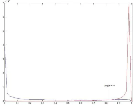
The distribution of the relative angles between posterior feature vectors belonging to the same class and the feature vectors belonging to the different classes is given in Figure 2. This distribution is approximated by the histogram of the cosine value of the relative angle between two feature
6
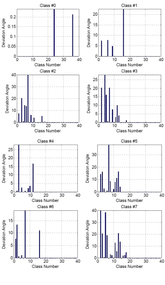
vectors. The intersection of the distribution of the same-class relative angles (left, blue plot) and different-class relative angles (right, red plot) is the optimal point above which features could be considered to belong to the different classes or to beg orthogonal. We could see that this intersection corresponds to the angle equal to 801. Hence, we defined a deviation angle from orthogonality as (80 – relative-angle) between the representatives. The results of this initial test to examine the characteristic of orthogonality are illustrated in Figure 3 for 4 of the classes. Complete results are given in appendix I. Since each class representative has a 0 relative angle with itself, the deviation angle is 80. Thus, the class with itself is excluded for plotting the figure in order to make it more illustrative. As it could be seen, the deviation angle in most of the cases is 0 or very small.
Finally, we defined a deviation angle from orthogonality as 80 – relative-angle between the representatives.
Figure 2. Histogram of the relative angle between same-class posterior feature vectors (left, blue line) and different-class (right, red line) posterior feature vectors
7
Figure 3. Initial test of orthogonality for classes 24-27. Each bar shows the deviation angle between the representative of the specified class and all other classes. The deviation angle for the specified class with itself is excluded to make the
figure more illustrative
To exploit this property we have to use a distance metric which has a geometric look into the posterior space. Therefore, the relative angle of the test sample with the training data is computed and the cosine function between these vectors is used as a distance measure. The nearest neighbors are then defined as the samples which lie in a hyper-cone with a specified angle originated from the test data. This angle could be interpreted as a look angle into the space. Then classification is done based on voting to find the dominating labels of training data which are geometrically in the nearby. By specifying the look angle, we have fixed the maximum value for the relative angle up to which the labels will be counted in kNN majority voting. This procedure eliminates the need to find the optimizing k value by cross-validation. Instead, the look angle is specified based on how restricting the orthogonality assumption is employed. For some of the vectors, there are not enough neighbors around when the look angle is fixed. These features are specified as uncertainties and are left undecided. We call this extension of the NN classifier as the Geometric Nearest Neighbor classifier or GNN.
Given the look angle by equation (4), the distance metric is the cosine function and corresponds to taking the scalar product of the vectors and then dividing by their norms as defined by
, cos ∑ .
∑ ∑
(5)
4. Experiments
4.1. Data and Features
Experiments are performed on TIMIT database, excluding the ‘sa’ dialect sentences. The training data consists of 3000 utterances from 375 speakers, cross-validation data set consists of 696 utterances from 87 speakers and the test data set consists of 1344 utterances from 168 speakers. The TIMIT database, which is hand labeled using 61 labels is mapped to the standard set of 39 phonemes as explained in [29], except in the way the closures are handled. In our case, when a
8
closure occurs before its own burst, the closure and the burst are merged (e.g. /tcl t/ → /t/). On the other hand, if a closure precedes any phoneme other than its own burst, the closure is mapped to its burst (e.g. /pcl t/ → /p t/). The speech signal is processed in blocks of 25 ms with a shift of 10 ms to extract 13 Perceptual Linear Prediction (PLP) cepstral coefficients every frame. These coefficients after cepstral mean/variance normalization are appended to their delta and delta-delta derivatives to obtain a 39 dimensional feature vector for every 10 ms of speech. A three layered MLP is used to estimate the phoneme posterior probabilities. The network is trained using the standard back propagation algorithm with cross entropy error criteria. The learning rate and stopping criterion are controlled by the frame classification rate on the cross validation data. In the basic system, the MLP has 351 input nodes corresponding to the concatenation of nine frames of 39 dimensional acoustic vectors, one hidden layer with 2000 units, and 40 output units (with softmax nonlinearity) in the output layer, each of them corresponding to different Phonemes.
4.2. Results and Discussion
In our experiments, the results of classification for kNN-KL, kNN-Euclidean, kNN-Bhattacharya and GNN are reported. Table 1 presents the best results achieved with kNN and the corresponding k values for each distance function. Table 2 gives the GNN classification rate for different look angles. Complete results for all look angles are given in appendix II. Results of the kNN with PLP features and Euclidean distance is 49.88% on the test set.
Table1. Local phoneme classification of posterior features with kNN and different distance functions KL Bhattacharyya Euclidean
68.51% 68.49% 68.34% k=200 k=150 k=260
Table 2. GNN classification rate for different look angles and the corresponding percentage of undecided samples Look_angle (deg.) %Classification Accuracy %Undecided Samples
0.5 79.7591 31.0083
1 76.4085 21.6652
1.5 74.5167 16.3881
2 73.2321 12.8594
We can improve the classification accuracy and determine the label for some of the GNN undecided samples by a method which we call it smoothing. In this method, each test sample after the initial kNN classification is looked in a window of a specified size with the test sample in the middle. The majority of the labels in this window is selected as the test sample new label. This is also a kind of post processing after kNN just to make the labels smoothed. Empirically, we selected the size of this window to be 5. However, larger windows up to 9 is successfully employed. Tables 3 and 4 give the performance of kNN after smoothing for all variations of distance metric. While improving the accuracy, the effectiveness of this method to reduce the percentage of undecided samples is quite noticeable.
Table3. Local phoneme classification of posterior features with kNN and different distance functions after smoothing KL Bhattacharyya Euclidean
68.82% 68.79% 68.6%
9
Table 4. GNN classification rate for different look angles and the corresponding percentage of undecided samples after smoothing
Look_angle (deg.) %Classification Accuracy %Undecided Samples
0.5 82.29 22.03 1 78.48 15.17 1.5 76.24 11.48
2 74.71 9.04
Comparing the results, the GNN approach which is based on a geometric look into the space and using the cosine function of the relative angle as the distance measure performs a high classification rate while specifying the uncertainties in data and leaving them to be undecided. The threshold for the number of neighbors is empirically decided. Based on our experiments, the accuracy rate improves exponentially as k increases from 1 to 40, then it becomes flat and no improvement will be obtained afterwards. Thus, we selected this threshold to be 40 with an interpretation of convergence of our classifier.
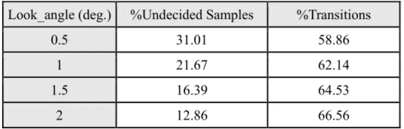
We are interested to examine closely where the uncertainties happen. An initial guess is that these features could be due to the side effect of coarticulation at transitions. We have tested this idea by determining the ratio of transition features between the undecided samples. The duration of transition is assumed to be 4 frames, 2 frames from each side. In general, this duration depends on the identity of the phoneme in the context and has to be estimated for each phoneme based on the training data in order to make the results more precise. Table 5 gives the ratio of transition in the uncertainties for different look angles.
Table 5. Ratio of transitions in the undecided samples Look_angle (deg.) %Undecided Samples %Transitions
0.5 31.01 58.86 1 21.67 62.14 1.5 16.39 64.53
2 12.86 66.56
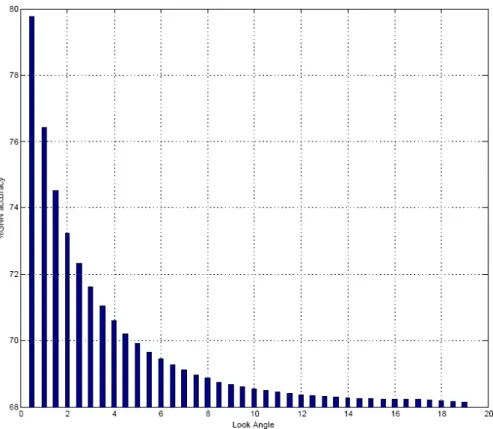
The evolution of the classification rate when the orthogonality assumption is relaxed is illustrated in Figure 3. As it can be seen, the accuracy decreases exponentially by increasing the look angle.
10
Figure 4. GNN performance for different look angles
Numerically, we can see that for the undecided samples the classification rate is always below 50%. This investigation strengthen the reliability and validity of our criteria for specifying the uncertainty in the given data.
kNN offers no obvious way to cope with uncertainty or imprecision in the data. This limitation has been already addressed as a major practicality problem in some applications (e.g. diagnostic) [30]. In the field of speech recognition, there are many sources which cause this ambiguity in features (e.g. co-articulation and pronunciation variation). Furthermore, the majority voting of kNN is sensitive to the phoneme distribution (i.e. a priori probabilities). The proposed approach provides a criteria to distinguish and specify ambiguous features which have to be dealt with by the higher level information modeled by the speech recognizer.
To closely see the classification performance for each phonemes, the confusion matrix is computed. Figure 4 shows this confusion matrix for the GNN classifier.
We have also compared the computational complexity of the proposed method with kNN using other distance metrics. We could see that GNN is the fastest. It is more than 10 times faster than kNN-KL and slightly faster than kNN-Euclidean and kNN-Bhattacharyya.
11
Figure 5. Confusion Matrix for GNN phoneme classification (angle=1)
As the final experiment, we investigated the empirical relationship between maximum-posterior probability and the percentage of frames correctly classified by GNN [1]. Figure 5 presents this plot for two of the angles. Roughly speaking, a linear relationship holds between maximum posterior probability (MAP) and the classification rate of GNN. This also shows how close is the performance of our method to the optimal Bayesian classifier.
Figure 6. Empirical relationship between maximum-posterior probability at the output of an MLP and the percentage of frames correctly classified by GNN (red stars). The plot is for an MLP trained on clean PLP features. As it can be seen,
12
5. Conclusion
In this paper we have investigated the use of kNN classifier for classification of local phonemes by posterior features. In this framework, we have used the cosine function between the feature vectors as a distance metric and we have proposed a new approach of classification based on NN rule. This idea is motivated by orthogonality characteristic of posterior features. Thus, the nearest neighbors are defined as the samples within a specific relative angle to the test data. Based on our experiments, the proposed approach yield 78.48% frame level accuracy while specifying 15.17% of features as uncertainties. Close examination of uncertainties reveals that many of them happen due to the phoneme transitions in speech signal which should be dealt with by higher level information modeled at the recognizer. They could be also considered to introduce new features which bring us closer to the orthogonality assumption and hence optimal posteriors.
6. References
1. Bourlard, H. and Morgan, N., Connectionist Speech Recognition – A Hybrid Approach, Kluwer Academic Publishers, 1994.
2. Mangu, L., Brill, E., and Stolcke, A., “Finding consensus in speech recognition: word error minimization and other applications of confusion networks”, Computer, Speech and Language, Vol. 14, pp. 373-400, 2000.
3. Abdou, S. and Scordilis, M.S., “Beam search pruning in speech recognition using a posterior-based confidence measure”, Speech Communication, Vol. 42, pp. 409-428, 2004.
4. Bernardis, G. and Bourlard, H., “Improving posterior confidence measures in hybrid HMM/ANN speech recognition system”, Proceedings of the Intl. Conference on Spoken Language Processing (Sydney, Australia), pp. 775-778, 1998.
5. Aradilla, G., Vepa, J., Bourlard, H., “An Acoustic Model Based on Kullback-Leibler Divergence for Posterior Features”, ICASSP 2007
6. Hermansky, H., Ellis, D., Sharma, S., “Tandem Connectionist Feature Extraction for Conventional HMM Systems”, Proceedings of the ICASSP, 2000
7. Hermansky, H. and Sharma S., “TRAPS Classifiers of Temporal Patterns”, Proceedings of Intl. Conf. on Spoken Language Processing (Sydney, Australia), 1998.
8. Hermansky, H., Ellis, D.P.W., and Sharma, S., “Connectionist Feature Extraction for Conventional HMM Systems”, Proc. IEEE Intl. Conf. on Acoustics, Speech and Signal Processing (Istanbul, Turkey), 2000.
9. Chen, B., Zhu, Q., and Morgan, N., “Learning long-term temporal features in LVCSR using neural networks”, Proc. Interspeech’04 (Korea), October 2004
10. Ikbal, S., Misra, H., Sivadas, S., Hermansky, H., and Bourlard, H., “Entropy Based Combination of Tandem Representations for Robust Speech Recognition”, Proc. Interspeech’04 (Korea), October 2004
11. Zhu, Q., Chen, B., Morgan, N., and Stolcke, A., “On using MLP features in LVCSR”, Proc. Interspeech’04 (Korea), October 2004
12. Niyogi, P. and Sondhi M. M., “Detecting Stop Constants in Continuous speech”, The Journal of the Acoustic Society of America, vol. 111, no. 2, pp. 1063-76, 2002
13. Aradilla G., Acoustic Models for Posterior Features in Speech Recognition, Ph.D. Thesis, Ecole Polytechnique Federal de Lausanne, 2008
14. Yang, H., van Vuuren, S., and Hermansky, H. “Relevancy of Time-frequency Features for Phonetic Classification of Phonemes”, Proceedings of International Conference on Acoustics, Speech and Signal Processing (ICASSP 1999), 1, 225–229.
15. Ikbal, S., Non-linear Feature Transformations for Noise Robust Speech Recognition, Ph.D. Thesis, Ecole Polytechnique Federal de Lausanne, 2004
16. Roweis, S. T., Saul, L. K., “Nonlinear Dimensionality Reduction by Locally Linear Embedding”, Science 22 December 2000, Vol. 290, No. 5500, pp. 2323 – 2326
17. Fukunaga K., Statistical Pattern Recognition by Statistical Recognition, Academic Press, 1990 18. Hunt, M.J., “A statistical approach to metrics for word and syllable recognition”, Journal Acoust.
13
19. Fix E. and Hodges Jr., J. L., “Discriminatory Analysis: Non- parametric Discrimination: Consistency Properties,” Report No. 4, Data set USAF School of Aviation Medicine, Randolph Field, Texas, Feb. 1951
20. Fix E. and Hodges Jr., J. L., “Discriminatory Analysis: Non-parametric Discrimination: Small Sample performance”, Report No. 11, USAF School of Aviation Medicine, Randolph Field, Texas, Aug. 1952
21. Cover, T.M., Hart, P.E., “Nearest Neighbor Pattern Classification”, lEEE Trans. Information Theory, vol. 13, no. 1, pp. 21-27, Jan. 1967
22. Elkan, C., “ Results of the KDD ’99 Classifier Learning Contest,” This paper presents a
methodology, neighborhood counting, Sept. 1999, http://www.cs.ucsd.edu/users/elkan/clresults.html 23. Hayashi, H., Sese, J. and Morishita S., “Optimization of Nearest Neighborhood Parameters for
KDD-2001 Cup ‘the Genomics Challenge’,” technical report, Univ. of Tokyo, 2001, http://www.tsujii.is.s.u-tokyo.ac.jp/GENIA/WS/PDFfiles/Morishita.pdf
24. Ikbal, S., Non-linear Feature Transformations for Noise Robust Speech Recognition, Ph.D. Thesis, Ecole Polytechnique Fédéral de Lausanne, 2004
25. Devijver, P. A. and Kitler, J., Pattern Recognition: A Statistical Pattern Approach, Prentice/Hall International, 1982
26. Ghosh, A. K., Chaudhuri, P., and Murthy , C.A., “On Visualization and Aggregation of Nearest Neighbor Classifiers”, IEEE Trans. on Pattern Analysis and Machine Intelligence”, vol. 27, no. 10, Oct. 2005
27. Ketabdar, H., Bourlard, H., “Hierarchical Integration of Phonetic and Lexical Knowledge in Phone Posterior Estimation”, ICASSP’08
28. Picard, B., “Improved Phone Posterior Estimation Through k-NN and MLP-Based Similarity”, Master Thesis, IDIAP 2009
29. Lee, K. F., Whon, H., “Speaker-Independent Phone Recognition Using Hidden Markov Models”, IEEE Trans. Acoust. Speech. Signal Process., vol. 37, no. 11, pp. 1641–1648, 1988
30. Denoeux, T., “A k-Nearest Neighbor Classification Rule Based on Dempster-Shafer Theory”, IEEE Trans. Systems, Man, and Cybernetics, vol. 25, pp. 804-813, 1995
14
Appendix I
Figure 2 in complete form: Initial test of orthogonality for all of the classes. Each bar shows the deviation angle between the representative of the specified class and the other classes
19
Appendix II
Tables 2 and 5 in complete forms: GNN classification rate for different look angles and the corresponding percentage of undecided samples and the percentage of transitions among undecided samples
Look_angle (deg.) %Classification Accuracy %Undecided Samples %Transitions
0.5 79.76 31.01 58.86 1 76.41 21.67 62.14 1.5 74.52 16.39 64.53 2 73.23 12.86 66.56 2.5 72.31 10.29 68.35 3 71.60 8.32 69.74 3.5 71.04 6.82 71.11 4 70.59 5.6 72.46 4.5 70.19 4.60 73.50 5 69.89 3. 8 74.42 5.5 69.64 3.13 75.4 6 69.44 2.60 76.41 6.5 69.26 2.12 76.65 7 69.1 1.75 77.5 7.5 68.97 1.45 78.72 8 68.85 1.19 79.61 8.5 68.75 0.96 80.12 9 68.66 0.78 80.65 9.5 68.60 0.63 80.94 10 68.54 0.51 81.02 10.5 68.49 0.40 80.98 11 68.43 0.31 81.73 11.5 68.4 0.24 83.03 12 68.36 0.18 82.74 12.5 68.33 0.13 80.43 13 68.32 0.1 78.79 13.5 68.29 0.07 72.16 14 68.27 0.05 67.36 14.5 68.25 0.04 57.65 15 68.24 0.02 38.64 15.5 68.24 0.01 27.04 16 68.22 0.01 17.78 16.5 68.22 0.06 14.07 17 68.20 0.00 8.15
20
Table 4 in complete form: GNN classification rate for different look angles and the corresponding percentage of undecided samples after smoothing
Look_angle (deg.) %Classification Accuracy %Undecided Samples
0.5 82.29 22.03 1 78.48 15.17 1.5 76.24 11.48 2 74.71 9.04 2.5 73.6 7.26 3 72.73 5.88 3.5 72.06 4.84 4 71.51 4 4.5 71.03 3.28 5 70.65 2.73 5.5 70.33 2.26 6 70.08 1.88 6.5 69.88 1.54 7 69.68 1.27 7.5 69.53 1.06 8 69.40 0.88 8.5 69.25 0.70 9 69.15 0.58 9.5 69.09 0.47 10 69.00 0.38 10.5 68.98 0.3 11 68.9 0.23 11.5 68.86 0.18 12 68.81 0.13 12.5 68.77 0.1 13 68.75 0.07 13.5 68.71 0.05 14 68.7 0.04 14.5 68.69 0.03 15 68.68 0.02 15.5 68.67 0.01 16 68.65 0.01 16.5 68.64 0.00 17 68.63 0.00
21
Appendix III
Description of one of the possible approaches for the use of temporal context in kNN:
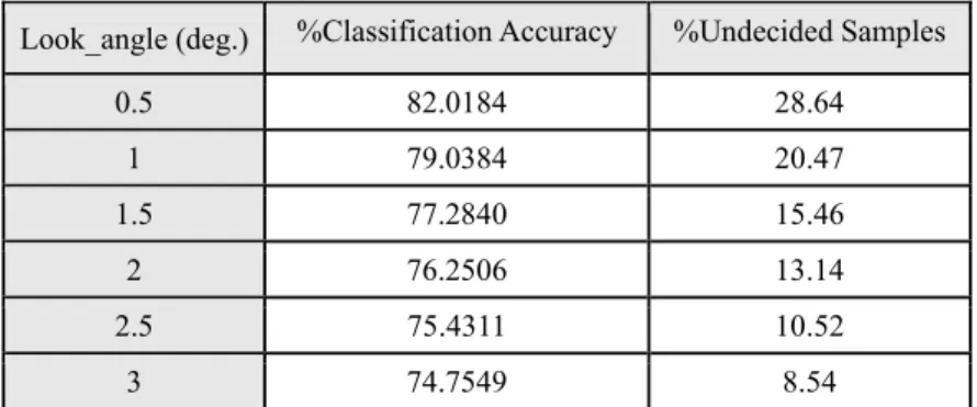
We carried out an experiment to boost the orthogonality of features by increasing the dimensionality using a concatenation of frames (larger temporal context). In this experiment, the test sample is investigated with a temporal context of 5 frames from the right and 5 frames from the left. Following the same procedure each training feature is also concatenated to 5 frames at its left and 5 frames at its right to form a larger feature vector. Then, the distance function between this new feature vector and all the training features is computed and classification is performed by GNN. It is clear that by considering such a large pattern, for many of the test samples there are not enough similar patterns at the specified neighborhood and these are left undecided; Therefore, for these samples we have formed a smaller context, this time with 3 frames at the right and 3 frames at the left. This procedure is continued until we reach to a test sample without any concatenation. Then we classified these remaining samples by the usual GNN approach. Our motivation to run this experiment was (1) to investigate the space in a higher dimension, (2) to use the information of a larger temporal context for classification and (3) the samples which are classified using a large temporal context are highly reliable and could result in a higher classification rate. Table 6 gives the frame level accuracy of GNN without considering the context. Table 7 presents the results of our method for using the temporal context. We know this test as running GNN with an adaptive use of temporal context.
Table 6. GNN classification rate for different look-angles and the corresponding undecided samples (cv data) Look_angle (deg.) %Classification Accuracy %Undecided Samples
0.5 82.0184 28.64 1 79.0384 20.47 1.5 77.2840 15.46 2 76.2506 13.14 2.5 75.4311 10.52 3 74.7549 8.54
Table 7. GNN classification rate for an adaptive use of temporal context (cv data) Look_angle (deg.) Classification Accuracy(%) Undecided Samples(%)
0.5 81.53 28.64 1 78.95 20.47 1.5 77.55 15.46 2 76.86 13.14 2.5 75.68 10.52 3 75.35 8.54