doi: 10.3389/fonc.2016.00149
Edited by: Adam Paul Dicker, Thomas Jefferson University, USA Reviewed by: Yaacov Lawrence, Sheba Medical Center, Israel Matthew T. Studenski, University of Miami, USA *Correspondence: James Coates [email protected]
Specialty section: This article was submitted to Radiation Oncology, a section of the journal Frontiers in Oncology Received:29 March 2016 Accepted:31 May 2016 Published:14 June 2016 Citation: Coates J, Souhami L and El Naqa I (2016) Big Data Analytics for Prostate Radiotherapy. Front. Oncol. 6:149. doi: 10.3389/fonc.2016.00149
Big Data Analytics for Prostate
Radiotherapy
James Coates1*, Luis Souhami2and Issam El Naqa3
1Department of Oncology, University of Oxford, Oxford, UK,2Division of Radiation Oncology, McGill University Health Centre, Montreal, QC, Canada,3Department of Radiation Oncology, University of Michigan, Ann Arbor, MI, USA
Radiation therapy is a first-line treatment option for localized prostate cancer and radiation-induced normal tissue damage are often the main limiting factor for modern radiotherapy regimens. Conversely, under-dosing of target volumes in an attempt to spare adjacent healthy tissues limits the likelihood of achieving local, long-term control. Thus, the ability to generate personalized data-driven risk profiles for radiotherapy outcomes would provide valuable prognostic information to help guide both clinicians and patients alike. Big data applied to radiation oncology promises to deliver better understanding of outcomes by harvesting and integrating heterogeneous data types, including patient-specific clinical parameters, treatment-related dose–volume metrics, and biological risk factors. When taken together, such variables make up the basis for a multi-dimensional space (the “RadoncSpace”) in which the presented modeling techniques search in order to identify significant predictors. Herein, we review outcome modeling and big data-mining techniques for both tumor control and radiotherapy-induced normal tissue effects. We apply many of the presented modeling approaches onto a cohort of hypofractionated prostate cancer patients taking into account different data types and a large heterogeneous mix of physical and biological parameters. Cross-validation techniques are also reviewed for the refinement of the proposed framework architecture and checking individual model performance. We conclude by considering advanced modeling techniques that borrow concepts from big data analytics, such as machine learning and artificial intelligence, before discussing the potential future impact of systems radiobiology approaches.
Keywords: radiotherapy, data mining, machine learning, big data, systems radiobiology
INTRODUCTION
Prostate cancer is the second most common cancer among men and is the fourth most common cancer overall (1). In Europe alone, prostate cancer is the most commonly diagnosed cancer in men and accounts for approximately one-quarter of newly diagnosed cases per annum (2).
Fractionated radiation therapy (radiotherapy) is a primary treatment method for prostate cancer patients with localized disease – approximately one-quarter of patients have some form of radiother-apy incorporated into their treatment regimen (3). The widespread acceptance of radiotherapy as a first-line treatment modality can be attributed to high rates of local control and acceptable levels of normal tissue toxicity (4,5).
Modern external beam radiation therapy (EBRT) delivery technologies, such as stereo-tactic body radiation therapy (SBRT) and volume-modulated arc therapy (VMAT), offer increased conformity and total dose while minimally damaging adjacent normal structures (6–8).
These advanced treatment tools generate vastly more amounts of treatment-related data than contemporary counterparts, such as three-dimensional conformal radiation therapy (3D-CRT). In terms of outcomes analysis, this can render quantitative modeling of treatment plans and retrospective outcomes exploration more complicated.
Historically, dose–volume metrics alone were used in an attempt to explain aberrant toxicities or biochemical relapses (9). Canonical examples of this include either hot spots in overlapping regions between PTV and normal structures that were thought to independently induce adverse normal tissue effects or, con-versely, suboptimal PTV coverage thought to be the main cause for inadequate local control (10). In recent years, however, it has been demonstrated that dose–volume metrics, while straightfor-ward to obtain and contributing significantly to the analysis of radiotherapy outcomes, are not the only determining factors of success in predicting radiotherapy outcomes (11, 12). This has been shown in prospective application of dose–volume metrics whereby such metrics have proven to provide limited classification performance (13,14). Aside from dose–volume data, the emer-gence of advanced imaging modalities and high-throughput “-omics” methods have led to the generation of enormous amounts of data that can similarly be used to predict outcomes.
The multi-dimensional space that EBRT-related biological, dosimetric and clinical variables span is referred to herein as the RadoncSpace. Two overarching predictive modeling approaches that exploit big datasets and search different sub-spaces of the RadoncSpace have surfaced in recent years: radiomics (use of imaging datasets for outcome prediction) (15) andradiogenomics (uncovering relationships between biological data and outcomes) (16). Pioneering application of these two techniques speaks to the ever-increasing application of data-mining techniques and big data analytics (the so-called “panomics”) to modern oncology (4). The specific objective of big data analytics in radiotherapy is to develop predictive models that capture underlying factors contributing to the development of selected endpoints without over-fitting noise or under-fitting trends. In line with the nature of big data and the heterogeneity of patient populations, a strict requirement of such modeling frameworks is that input datasets must be large enough to include variability, which accurately reflects the underlying patient population. Otherwise, resulting models can suffer from poor prospective prediction performance. Clinically, it has already been demonstrated how such models could be used to better inform patients of treatment-associated risks. Namely, by integrating outcome models into treatment planning systems (TPSs) and recommending dose-escalation or dose-reduction (11). Given the potential future impact of outcome models in the clinic, the selection of tools and models for the fabrication of a predictive framework must be chosen carefully in a way to facilitate identification of optimal models.
In this work, we focus our attention exclusively on outcomes associated with EBRT; however, the presented modeling tech-niques are easily generalizable to any dose distribution. In this work, we briefly review the radiobiology of prostate cancer as a basis for understanding the theoretical underpinnings of ana-lytical outcome models. Anaana-lytical models attempt to predict radiation-related toxicities by formalizing abridged versions of the
biological processes by which selected endpoints become man-ifest. Subsequently, we discuss big data and data-driven model-ing approaches based on techniques previously used successfully for exploring outcomes in radiotherapy. In contrast to analyti-cal models, data-driven models are entirely empirianalyti-cal in nature, potentially making them more robust albeit more difficult to analyze or interpret. We then consider techniques that optimize model parameters in order to maximize model robustness and prevent under-/over-fitting, which are two common pitfalls in big data outcome modeling. The article concludes by presenting modeling techniques based on advanced artificial intelligence as well as on systems theory.
PROSTATE CANCER
Pathology
Adenocarcinoma of the prostate is the most common histopatho-logical type of prostate malignancy and typically arises in the peripheral zone (17). Up to one-half of men present with prostate cancer at time of autopsy although tumors identified in many of these cases are typically small, impalpable, and of low grade (18).
Prostate tumors are known to have remarkable biological het-erogeneity from patient to patient and even across tumor volumes (19–21). The metastatic potential of prostate cancer is similarly variable and is furthermore reflected in the wide variation in overall survival rates for those with localized disease at time of diagnosis (21). Notably, the high degree of heterogeneity makes standardization and characterization of prostate adenocarcinoma phenotypes challenging and institution specific.
Basic Radiobiology
Theα/βoriginates from the linear-quadratic (LQ) formulation of in vitrocellular survival experiments (Eq. 1):
SF=e−(αD+βD2) (1) where SF is the surviving fraction after a dose (D). The coefficient
α[Gy−1] in front of the linear dose term (D) relates to single-hit inactivation and theβ[Gy−2] coefficient pertains to the expected rate of double-hit (two-track) cellular inactivation (22,23). The
α/βratio taken from the LQ model allowed numerous funda-mental radiobiological questions to be answered quantitatively. It remains a relevant parameter in radiotherapy today due to its clinical significance as a measure of tissue-specific fractionation-sensitivity.
It is well known that prostate cancers are relatively slow-growing malignancies with lowα/βratios (24–27), unlike most malignancies. When used in the context of biologically effective dose (BED) (Eq. 2), the low prostateα/βratio (~1.5 Gy) translates to a high sensitivity to fraction size:
BED=D· ( 1+ d α/β ) (2) whereDis the total dose of the radiotherapy regimen anddis the fraction size. Furthermore, since theα/βratio for prostate cancer
is lower than that of normal tissues (~3 Gy), an improved thera-peutic ratio can be expected using hypofractionation (28–30).
In 2013, Vogelius and Bentzen performed a meta-analysis of 1965 patients derived from five separate studies (31). In line with pioneering work by Fowler and colleagues (25), they showed that prostate cancers do indeed have an exceedingly low α/β ratio. Interestingly, after accounting for changes during treatment, their estimate of α/β increased. This may indicate that the α/β for prostate tumors changes throughout the course of radiotherapy treatment, probably due to subpopulation selected induced by radiotherapy itself.
Although α/β has provided insight into radiobiology of prostate cancer, it remains unclear how relevant the ratio is in cases of modern EBRT delivery, such as high-dose hypofractionated SBRT regimens, mixed-modality treatments (photon with proton boost) or when using charged particles, such as carbon ion, all of which are becoming increasingly popular treatment options for prostate cancer. In such cases, aggregation of large-scale datasets serving as inputs to big data analytics may provide more use-ful insight either as a supplement or as a substitute to classical paradigms in radiobiological modeling.
TYPES OF OUTCOMES
Toxicity outcomes in radiotherapy can be segregated into two categories: acute (effects observed within 3 months after the ter-mination of radiotherapy) and late (effects that manifest after the 90-day cutoff). Furthermore, normal tissue damage can be segregated by site; in prostate radiotherapy, normal tissue side effects manifest themselves most frequently as one or more of gastrointestinal (GI) toxicities, genitourinary (GU) toxicities, or erectile dysfunction (ED).
Acute (Early) Outcomes
Acute effects due to normal tissue damage from ionizing radi-ation in prostate cancer radiotherapy regimens include GI/GU symptoms. Acute symptoms are most often transient, self-limiting events in that they appear and resolve within a matter of weeks without contributing significantly to severe or long-term morbid-ity, although some consequential late effects in prostate radiother-apy have indeed been recorded (32–34).
A 2015 review article by Drodge et al. compiled the results of 22 prospective hypofractionated trials completed between 2001 and 2013 (35). Using the RTOG/EORTC toxicity grading scheme and including studies that used different treatment modalities and schedules, the authors concluded that Grade 3 acute toxicities, on the whole, affect less than 10% of prostate patient cohorts receiving hypofractionated EBRT. Furthermore, Grade 2 toxicities affected under half of patients. The study also expanded upon the practical challenges in interpreting outcome data from independent trials that may use different grading schemes or endpoints.
Proton therapy is becoming more common in modern times for use in treating prostate cancer (36). Studies have shown that the frequency of acute effects with proton for prostate cancer is not significantly increased over that of conventionally frac-tionated photon therapy regimens (37,38). One dose-escalation study with 85 prostate cancer patients using proton doses up to
82 Gy-equivalent (GyE) yielded acute toxicity levels comparable to photon radiation (39).
Late Normal Tissue Endpoints
Radiation-induced late normal tissue damage consists of toxicities that occur>90 days after completion of radiotherapy. Late tox-icities can range from mild, moderate, severe to life-threatening requiring immediate intervention. They are categorized as either GI or GU effects and many retrospective studies report only these outcomes; however, sexual dysfunction is also considered herein. Unfortunately, the full pathophysiology of the radiation-induced manifestation of ED has yet to be fully elucidated.
The difficulty in assessing late toxicities is that often times no quantitative physiological evidence exists or can readily be obtained. Grading schemes have been developed to resolve such issues. Grading schemes require physicians to assign integer val-ues to the radiation-induced side effect based on selected criteria. Some schemes utilize self-scoring questionnaires, while others rely on grades assigned by attending oncologists. Interestingly, several groups have sought to explore the correlation between different scoring schemes using a single set of data in order to explore what role grading schemes have on incidence rates of toxicity (40–42). Such works bear significance for the use of big data analytics as many frameworks utilize supervised learning techniques that rely on the accuracy of outcome measures.
Local Control Endpoints
It is estimated that overall approximately one-third of prostate cancer patients experience some type of biochemical relapse within the first decade after completion of their EBRT treatment regimen (43). In reporting local control outcomes, clinical studies typically do so according to specific criteria, such as the ASTRO-RTOG Phoenix definition of local biochemical failure (44). Guide-lines often include prostate serum antigen (PSA) scores although derivatives of simple PSA scores have also been considered, such as PSA doubling time (43). However, it should be noted that a rising PSA does not always indicate a local failure and it can antedate the diagnosis of metastatic disease for many years; thus, caution should be exercised when using it as a surrogate for local failure endpoint.
DATA TYPES
Dose–Volume Metrics
Typical dose–volume metrics used in outcomes modeling include dose to a given volume or volume of tissue receiving at least a particular dose. These parameters can be readily extracted from dose–volume histograms at the treatment planning stage. Physiological changes, such as weight gain/loss or changes in tumor composition or anatomical position, may take place during treatment and, thus, dose delivered may not necessarily reflect biologically absorbed dose. It is likely that dose–volume variables could have their predictive accuracy improved by incorporating intra-fractional computed tomography (CT) scan changes, as has been considered in literature (45).
The equivalent uniform dose (EUD) (46) is a dose–volume metric that can be used to describe inhomogeneous dose
distributions. The generalized EUD (gEUD) (47) is a further extension used for normal tissues of interest (Eq. 3):
gEUD= ( ∑ i viDai )1/a (3) where the variablesviis fractional volume for the tissue exposed
to dose Di, the parameter ais a factor relating to the volume
effect of a given tissue type. These two metrics appear oftentimes in analytical outcome models as they serve as excellent tools to summarize dose distributions across volumes.
Clinical Parameters
Clinical data can be parameterized and used to investigate covari-ates of interest. An example in the case of prostate cancer is in patients receiving anti-coagulant therapy and presenting with rectal bleeding (RB) late in their follow-up period, which can otherwise easily be mistaken for a late toxicity. Another case is the combined use of androgen deprivation therapy (ADT) since ED can be a side effect of ADT alone and thereby lead to an increased prevalence of late ED in a given prostate patient cohort.
Spatial Parameters
Spatial dose–volume histograms (zDVHs) can be used to compare spatial treatment planning information to outcomes (48–50). The advantage of incorporating spatial information is that it provides modeling frameworks information about the location of dose extremes and, thus, mitigates having to rely solely on approaches based on volume-averages (or gEUD). This reduces the risk of under- or over-valuing the contribution of hot or cold spots. Spa-tial data can also provide information related to the contribution of hot spots in accessory structures, for example, in the case of rectal contour overlap with the PTV.
Biological Variables
Several types of biological variables have been used previously in attempting to elucidate mechanisms by which prostate radio-therapy toxicities become manifest. The most popular class of variables found in literature today is related to genetic mutations. Additionally, work has been performed on exploring the role of epigenetics (51) and transcript expression levels (52) in long-term radiotherapy outcomes.
Genetic Variables
Given the relatively disappointing prospective predictive power of singular classes of genetic variables on their own (53–56), it is likely that modeling frameworks will need to allow for several types to be incorporated in a given model in order to maximize prospective classification performance.
Single-nucleotide polymorphisms (SNPs) consist of single-nucleotide changes. Their presence in certain genes or regula-tory regions has been shown to be well correlated with prostate radiotherapy-related outcomes (52,54,57,58). This is probably due to altering functional transcripts or protein confirmations after translation.
Further to SNPs, copy number variations (CNVs) have recently been of increasing interest to the radiotherapy community (59).
CNVs reflect the number of copies of a particular gene and are, therefore, larger structural genetic mutations than SNPs. This could mean that larger changes in a given genome could be seen with CNV changes.
In our previous work, we have shown the value of integrat-ing CNVs alongside SNPs (of the same gene) together with dose–volume metrics (60). Specifically, we have demonstrated that changes in the gene concentration of DNA repair gene XRCC2 can predict severe (Grade 3) late RB for hypofractionated prostate patients treated with 3D-CRT. More importantly, the resulting radiogenomic models led to increased predictive power as compared to using either type of genetic variable alone. We, furthermore, demonstrated that the improvement using SNPs and CNVs is not limited to data-driven frameworks but could also be applied to analytical models. These results indicate that different genetic mutations in the same gene may contribute similarly to a given outcome. If proven to be the case, it is likely a result of outcome scores being limited snapshots of complex pathophysio-logical events reflecting more than one biopathophysio-logical alteration. Integrating Genetic Variables in Outcome Models
In the case of data-driven modeling, genetic parameters can be considered as independent variables and regressed along-side clinical risk factors and dose–volume metrics. For analytical models, the method in which genetic parameters are integrated depends on the nature of the model at hand. In 2006, two groups showcased how dose-modifying factors (DMFs) extracted from clinical risk factors could be used to stratify standard analyti-cal models and thereby generate “mixed” data-type models (57,
61). In 2013, Tucker et al. expanded this approach to include SNPs using an approach easily generalizable to any biological variable and demonstrated significantly improved classification performance (62). Rancati and colleagues further extended this approach using clinical risk factors for Logit and EUD mod-els (63), from which our group drew inspiration in developing radiogenomic models using biological, clinical, and dosimetric variables (60).
Other Biological Variables
Epigenetics
The importance of epigenetic alterations to the genetic code has not by any means been understated by the scientific community in recent years (64–67). However, the significance of epigenetic modifications in radiotherapy remains to be fully understood. Research related to epigenetics and radiotherapy could be compli-cated by the fact that mounting evidence implies that radiotherapy itself can induce epigenetic changes (67).
Thus far, thousands of differentially methylated regulators have been identified in many cancer types thanks to epigenome-wide association studies (EWAS) (68). Differentially regulated pro-moter may serve as novel biomarkers to predict risk of biochemi-cal relapse or serve as indicators of normal tissue radiosensitivity. In prostate cancer specifically, wide-ranging hypo- and hyper-methylations have been identified that correlated with early-stage carcinogenesis and aggressive tumor phenotypes (69,70). Efforts are underway to generate an epigenetic code (71–73), which may facilitate the ability to perform and interpret EWAS
results as well as provide a new class of input data for outcome models (74).
High-throughput Proteomics and mRNA Expression Levels Numerous methods used to quantify large numbers of biological factors have been pioneered and introduced into mainstream biol-ogy research within the last decade. These technologies include well-characterized microarrays and proteomic analysis technolo-gies that can quantify the levels of expression of up to tens of thousands mRNA transcripts or proteins in a single sample.
After generating large quantities of data, high-throughput modeling frameworks can be used that are able to deal with large numbers of variables (75). This approach has been used successfully in clinical oncology to stratify tumor phenotypes and estimate prognoses to help guide optimal therapeutic regimens (76–78). In the case of radiation oncology, high-throughput data have yielded several multi-gene signatures for hypoxia (79–81).
The challenges of utilizing a large number of variables in outcome models are well summarized by the multiple testing dilemma: too few samples relative to a large number of variables being tested can lead to spurious correlations. Even after utilizing simple supervised learning algorithms to pre-process the data, the number of mRNA transcripts that a single microarray experiment can yield is often in the thousands (82). This issue can be mitigated by large-scale validation studies but these are expensive, time-consuming and patient accrual can limit achieving the necessary sample size.
Alternatively, methods in artificial intelligence are becoming increasingly popular to explore the complex, hidden relationships between outcomes and biological variables (83). In contrast to brute-force estimating of correlations, machine-learning tech-niques in artificial intelligence have the ability to process highly structured, high-dimensional data while controlling for over- and under-fitting by drawing on methods from control, probability, and information theory.
MODELING TECHNIQUES
Risk Quantification
The likelihood of obtaining local control is quantified mathemati-cally by tumor control probability (TCP). TCP is a probability that indicates chances for success of a treatment according to a par-ticular endpoint, usually long-term control. Many studies using TCP-based approaches have shown that cancer cellsin situhave complex, high-dimensional repopulation kinetics when exposed to ionizing radiation and/or chemotherapy (84–87). Such kinet-ics can lead to complex models and be dependent upon several factors, such as repair capacity, quality of radiation, fractionation scheme, and surrounding microenvironment (88).
In the case of normal tissue side effects from radiotherapy, risk is quantified via normal tissue complication probability (NTCP). NTCP values can be tailored to each individual treatment reg-imen to reflect the risk of a given side effect. Conventionally, such frameworks were limited to dosimetric data; however, it is now understood that late normal tissue toxicities are furthermore functions of a variety of biological, physical, and clinical factors (16,89).
Analytical Modeling
As previously described, models of the analytical class are based on simplified theoretical mechanisms of action radiobiological interactions. They include some level of mechanistic insight into a specific mechanism by which radiotherapy outcomes become manifest and are, therefore, also referred to asmechanistic models.
Tumor Control Probability
Cells that can lead to tumor growth are termed tumorigenic stem cells or cancer stem cells. These cells are, in theory, the primary targets of anti-cancer therapies. The probability that a given treatment will induce eradication of cancer stem cells for a given patient is mathematically given by the TCP.
The Linear-Quadratic
The LQ model has gained popularity in literature since it follows survival closely at conventional doses of radiation. Furthermore, the model provides a simplified theoretical basis for how radiation induces cellular deactivation: radiation tracks interacting with DNA can induce severe damage on its own (αcomponent) or can combine with another track to increase density of damage (β
component).
Questions have, however, arisen to the relevance of the LQ model for more modern treatment regimens, such as SBRT or charged particle therapy. It has been shown that the LQ model begins to deviate significantly from experimental data begin-ning at or around 6–8 GyE (22, 90, 91). Practically speaking, this does not affect conventional treatment regimens utilizing 2–3 Gy fraction sizes; however, the LQ model may predict effects of hypofractionation regimes poorly. One such example is the carbon ion lung trial in Japan whereby single fractions of 50 GyE were delivered (92). Furthermore, when considering casesin vivo, the standard LQ model does not take into account repopulation kinetics of cancer cells during intra-fraction periods, rendering it approximate at best (93).
Modified LQ Models
Modified versions of the canonical LQ model have been proposed to address some of the aforementioned shortcomings. Examples include generalized versions that have been further parameterized to account for repopulation (94), mixed radiation qualities (95), tumor heterogeneity, arbitrary or variable dose-rates (91), cell death mechanisms (96), and others able to take into account more than one of the aforementioned parameterizations (97).
In the case of charged particle therapy, the theory of dual radiation action (TDRA) predicts an increased linear component of LQ-modeled cell kill (α) over the quadratic component (β) (98). Indeed, it has been shown that βremains relatively stable in comparison to the variation ofαacross linear energy transfers (LETs) (99). Consequently, by considering the relative biological effectiveness (RBE) between a given high LET radiations and clinical energy photons, TDRA predicts that RBE will reach a minimum (RBEmin) at very high doses, while at low doses RBE
will reach an intrinsic maximum (RBEmax) (100). In practice, it
has been observed that both parametersαandβvary with LET. Thus, a modified LQ model has emerged that RBEminand RBEmax
are taken into account by further parameterizing the high-LETα
andβvalues (Eq. 4a, b).
αΗ=αL·RBEmax (4a)
βH=βL·RBE2min (4b)
whereαH and αL refer to α components of the high and low
LET radiations, respectively, andβHandβLrefer to the quadratic
components of the high and low LET radiations, respectively. In considering high-dose per fraction, such as those delivered by a SBRT prostate radiotherapy plan or charged particle therapy, the modified LQ model first proposed by Sachs et al. in 1997 (101) and extended in 2004 by Guerrero and Li (91) has been demonstrated to fit survival data well (Eq. 5a, b).
SF=e−αD−β·G(λT)·D2 (5a) G(λT) =2(λT+e−λT−1)/(λT)2 (5b) whereλis the repair rate and T is treatment delivery time while the other parameters are taken from the standard LQ model. G(λT) is the dose protraction factor that specifies the contribution of misrepair to lethality (which is reduced at high, acute doses). Using this formulation of the LQ model, the large differences in cellular survival observed between predicted and experimental data are practically eliminated up to doses of ~30 GyE (91).
Review articles by Jones and Dale (23) and Zaider and Hanin (102) have elegantly summarized and discussed additional models and can be consulted for further details.
Normal Tissue Complication Probability
The objective of NTCP models is to gage the risk of inducing particular normal tissue effects, such as severe RB in the case of late prostate radiotherapy. A plethora of modeling techniques have been proposed for such purposes (103–105), some of which are described in more detail below.
Lyman–Kutcher–Burman
The most readily applied analytical method for generating NTCP values is through the Lyman–Kutcher–Burman (LKB) approach (106) (Eq. 6a,b). NTCP(D,D50,m) = √1 2π t ∫ −∞ e ( −u2 2 ) du (6a) wheret= EUD−TD50 m·TD50 and TD50(V) = TD50(1) Vn (6b)
wheremis the slope of the best-fit NTCP sigmoid,TD50(1)is the
dose at which NTCP=50% for a specific endpoint, andTD50(V)
is the tolerance dose for a given partial volume with tissue-specific volume exponentn. Simply put, the LKB model stratifies patient risk according to how much larger or smaller their EUD is relative to the TD50. The EUD is a three-dimensional DVH reduction
technique according to Eq. 7. EUD= ( ∑ i vi·D 1 a i )a (7) where parameterais 1/n, andDiandviare the dose and partial
volume, respectively, according to each DVH segmenti. Expan-sions and more intricate variations of the canonical LKB model can be found readily throughout literature (57,60,62).
Binomial Models
The Critical VolumeFunctional subunits (FSUs) are thought to be fundamentally underlying structured subunits housing numerous cells in a given tissue. Perhaps the most readily available example is the crypt subunit in the GI tract that together forms the organ. FSUs have varying properties, shapes, and sizes and are tissue type specific. Such variation can be exploited by the critical volume (CV) model (Eq. 8) to account for the differences in radiation response between different tissue types (107).
Pt= ( N t ) PtFSU(1−PFSU)N−t (8)
where the first term is the binomial coefficient ofNandt. PFSUis
the probability thattofNsubunits will be deactivated by ionizing radiation. Accordingly, the chance ofMor more subunits being deactivated in a single exposure can be calculated according to:
P= N ∑ t=M+1 Pt= N ∑ t=M+1 ( N t ) PtFSU(1−PFSU)N−t. (9)
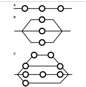
Two major classes of tissue exist in the context of FSUs
(Figures 1A,B): serial and parallel. Organs that are serial can have
their function compromised by exposure of a limited volume (a “critical volume”) to a given dose, e.g., colon, spinal cord, brain stem. Note that the output of a serial organ is not a sum of its internal components as it is in the case of parallel organs. Thus, for parallel-type tissues, catastrophic damage to one part of the underlying physiological architecture does not risk the collapse of the organ itself, e.g., liver, skin. In reality, every tissue has a mix of both serial and parallel structures, a concept referred to “complex” FSU arrangement (Figure 1C), although some tissues are more one type than the other.
Interestingly, it has been shown that the LKB model can be derived upon reformulation of the CV model. This implies that the LKB model has a basis relating to FSUs (108).
Prior to mainstream applications of data-driven modeling tech-niques, modifications to the CV model (109,110) and extensions of the FSU concept (111) were shown to be useful. Applications of the CV model in prostate cancer to predict late endpoints relat-ing to bladder, colon, bowel, penile bulb, and rectum have been performed; however, their usefulness in practice has been limited compared to models identified using contemporary data-driven modeling approaches (112,113).
Relative SerialityThe relative seriality model for NTCP modeling was developed in order to consider and exploit arbitrary combina-tions of serial and parallel FSU arrangements (114). In such cases, risk of normal tissue damage is given by the following equation:
NTCP(D,V) = [ 1− ( 1−P(D)S )V/Vref]1/s (10) where the exponent V/Vrefis the fraction of volume that is being
irradiated to the given dose,D, and the parameterSrelates to the degree of seriality of the organ at risk – nearly 0 in the case of highly parallel structures and higher for mixed or serial structures.
FIGURE 1|Arrangements of functional subunits in (A) serial formation, (B) parallel formation, and (C) complex, or mixed, formation. FSUs are functional compartments of a given organ. The concept of FSUs underpins many models for modeling NTCP, including the critical volume and relative seriality models.
The functionP(D) is the value of risk and can be derived via Poisson statistics:
P(D) =e−No·S(D) (11)
whereNois the number of FSUs and the function S(D) is the
probability of a given FSU in the order of interest to survive irradiation to doseD.
Data-Driven Modeling
Data-driven approaches to modeling are often referred to as phenomenological or statistical techniques. Models generated by such frameworks are based on empirical combinations of obser-vations and are, thus, generally more robust than their analytical counterparts.
When considering dose–volume metrics alongside clinical and genetic risk factors, the number of variables can quickly become overwhelming and so data-driven modeling frameworks often include steps that seek to optimize and pre-process input data.
The most frequently employed approaches to data-driven mod-eling in radiotherapy are regression-based techniques. Regres-sion link functions are typically chosen to be sigmoidal in order to achieve the non-linear dose–responses seen experimentally. Advanced methods in artificial intelligence that are able to handle non-linear data more readily are discussed later in this section. Such methods are becoming increasingly popular due to superior prospective classification performance in many areas of oncology (15,115,116).
Several review articles discussing the shortcomings and advan-tages of data-driven modeling can be found elsewhere in the literature (11,117,118).
Probit- and Logit-Based Regression
Link functions can be used in tandem with regression frameworks to fit either TCP or NTCP data. The use of an inverse-logit (Eq. 12) or -probit (Eq. 13) are examples of such functions.
π(Xi) =Φ(g(Xi)) (12) π(Xi) = e g(Xi) 1+eg(Xi) = 1 1+e−g(Xi) (13)
where g(xi) is the generalized linear model (GLM) formulation of
the input variables: xi:
g(Xi) =β0+
s
∑
j=1
βjXij,i=1, . . . ,n,j=1, . . . ,s (14)
whereβcoefficients are estimated according to maximum likeli-hood estimation (MLE).
Historically, the logit function has been employed more often than the probit function because of ease of use and mathematical simplicity.
In terms of interpretation in the context of prostate radiother-apy, data-driven models have the added benefit of being able to handle multiple types of data while independently stratifying the contribution of specific variables. This can again be contrasted with analytical models wherein parameters need only be estimated rather than having to entirely develop the model itself.
Artificial Intelligence (Machine Learning)
Techniques in artificial intelligence applied to outcome modeling consist of time-invariant statistical methods that are able, to a degree, to mimic selected human hallmarks. Artificial intelligence frameworks must first be able to learn (training phase) a pattern and then produce models that are able to recognize the pattern in a prospective setting (testing phase).
Success using artificial neural networks (ANNs), one of the major classes of artificial intelligence, has been achieved in learn-ing and reproduclearn-ing critical elements from the fields of speech pathology and handwriting recognition, both of which require complex recognition. Each node on a neural net indicates a func-tion and, as such, refers to a transformafunc-tion. In this context, a neu-ral network itself carries no values without input data. In oncology, neural networks have also been used successfully although they have yet to be used prospectively (119–121).
Much criticism has arisen in recent years on the application of ANNs to prediction problems in oncology (122). Single hidden layer ANNs are universal function approximators, meaning that they can theoretically represent any function, which is defined by their topology and weighting values. This may lead to the fitting of implausible functions to datasets yielding uninterpretable and simply illogical results.
Feed Forward Neural Network
Feed Forward Neural Networks (FFNNs) (Figure 2) do not include any recurring nodal inputs (“memories”) and are used frequently in basic pattern recognition problems. FFNNs are fully defined by their architecture such that arrangements of nodes into different topologies can induce different system responses. The
FIGURE 2|Diagram of a feed forward neural network (FFNN). None of the nodes within the network are recursive.
user decides what topology to employ for a given FFNN during the training phase although some have demonstrated the feasibility of using separate optimization algorithms to optimize network architecture itself (123–125). In radiation oncology, attempts have previously been made to utilize FFNNs for their ability to classify highly non-linear data (126,127).
Each node of a FFNN represents a function with one or more inputs. Inputs from previous nodes are transformed according to an activation function. Examples of commonly used activation functions are logit or probit functions. Other functions, such as the radial basis function (RBF), can also be used if data are suspected of originating from a specific type of distribution. After transformation by activator functions, outputs from nodes are stratified by weights. Such weights are the elements of the FFNN that are trained when building a FFNN. Training of nodal weights is relatively straightforward albeit time-consuming. Thedelta rule can be used via back-propagation to adjust node input and output weights until classification performance is optimized. Datasets for training can be used all at once (batch training) or can be segregated into pattern-based subgroups (sequential training).
One shortcoming of FFNNs is that extraction of relationship data from within them can be notoriously difficult, if not, impos-sible. Information for final output nodes is reliant on previous inputs and outputs and, therefore, can become extremely mathe-matically complicated. This disadvantage is somewhat of a trade-off given that the only time-intensive procedure is training of node weights, after which the network can be used for real-time classification. Validated FFNNs are, therefore, indeed amenable to clinical implementation.
At least one group has demonstrated the applicability of ANNs in predicting late RB and in fact demonstrated improved pre-diction performance over and above that of regression-based approaches (123). Their findings exploited a genetic algorithm for optimizing inputs into their neural network and, furthermore, leveraged multiple cross-validation phases.
Generalized Regression Neural Network
In contrast to the FFNN, the generalized regression neural net-work (GRNN) is a probabilistic neural netnet-work developed in 1991 and can, overall, be thought of as a best-fit estimator (128). The technique generalizes canonical regression by not being limited to
a specific function (e.g., in linear regression) but instead expresses an empirical regression function as a probability density deter-mined using a technique known asParzen window estimation. To accomplish this, the technique utilizes the joint probability of the input vector(s) and the outcomes to calculate conditional prob-abilities and expected values. These values are used to estimate the generalized regression of the outcomes onto the input data. The joint probability of the input vectors and outcomes can be estimated via non-parametric estimators if not known outright.
In the context of training, the advantage of GRNNs is that they avoid having to backpropagate error to fine tune nodal weights, which is computationally expensive and time-consuming. Back-propagation is mitigated by dealing with probability distributions rather than discrete raw input data. This means that one-pass of the framework with training data is sufficient to estimate parameter weights. Previous work by our group has shown that GRNNs can outperform FFNNs when it comes to prospective applications in radiation oncology (129). This is likely a result of the probabilistic nature of nature and/or biological variables across a patient cohort.
Kernel-Based Methods
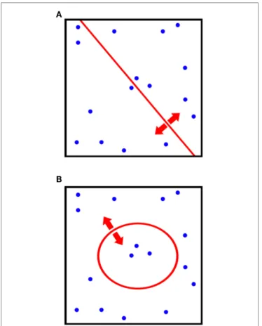
Kernel-based approaches to classification problems are based on clustering data according to non-linear combinations of variables (such as hyperplanes) in order to separate data. Oncology data are oftentimes highly non-linear, which gives motivation to explore the application of such a technique. Kernel methods seek to maximize distances between clusters that have undergone linear transformations. In this sense, the technique is a non-linear analog of Fischer’s non-linear discriminant (FLD) analysis and principle component analysis (PCA) (Figure 3).
The most prominent member of the kernel-based learning family is the support vector machine (SVM). SVMs utilize support vectors that are formulated according to the most difficult to separate data and, therefore, are relied upon by the method in order to select an optimum classifier. By formulating the distance maximization problem between support vectors as a quadratic programing problem, a computationally efficient SVM formula-tion can be described by the following predicformula-tion funcformula-tion:
f(X) =
ns ∑
i=1
αiyiK(Si,X) +αo (15)
where the number of support vectors is given by ns, K is the
kernel transformation, andαi is the coefficient determined by
quadratic programing. Further details on kernel-based methods can be found readily in the literature (130–132) or in our previous work (133).
Systems Biology Approach
The concept of an integrated systems approach is that of under-standing a given problem in terms of all of its components together, i.e., taking a “system-wide” view. This can be contrasted with a reductionist approach whereby each component of a system is looked at separately. A given system can be thought of having four principal components: structure (network topology), dynam-ics (time evolution of system), control (response and regulatory
FIGURE 3|Comparison of the differences in classification procedures of (A) canonical principle component analysis (PCA) and (B)
kernel-PCA. By utilizing a kernel transformation, non-linear thresholds can be used to separate and classify data.
systems), and design (operational parameters or rules) (134). In applying a systems approach to biological and physiological systems, much insight could be gained that would otherwise be extremely challenging to extract using phenomenological models (135–137).
The biological effects induced by ionizing radiation are initiated at the atomic level in the form of free radical reactions. Free radical interactions occur rapidly and induce cascades of molec-ular responses, such as inflammation, which ultimately lead to recruitment of a variety of different molecular factors (138). Ulti-mately, over time, cellular responses can manifest themselves as clinical effects that are recorded as treatment outcomes, including toxicities. Much mechanistic insight and predictive power would be derived from a model that is able to combine these different organizational levels and related biophysical properties. Unfortu-nately, however, such a model requires expansive radiobiological knowledge spanning very different time and length scales, thus making the problem inherently complex.
In a related category, graphical models have been shown to be of use in radiation oncology as they can capture complex relationships between relevant factors and inter-dependencies between variables (Figure 4) (139,140). Graphical models differ from aforementioned neural nets in that each random variable is represented by a node within the system and forms part of
FIGURE 4|Schematic diagram of relationships in a three-node graphical model with two recursive relationships. Note how the model does not have a singular output as the outputs from the middle node are used as inputs. In contrast to artificial neural networks (ANNs), graphical models can take into account how variables are related via such conditional dependences.
an intricately connected web. The web simulates conditional probability relationships making this class of algorithm classified as a structured prediction technique as oppose to clustering or regression (discussed previously). In previous work, our group has shown good classification performance using a graphical Bayesian network in predicting radiation-induced pneumonitis (116).
MODEL ORDER ESTIMATION
Resampling Techniques
Frameworks that exploit resampling can be used to make estimates of model orders, parameters, or errors. In all cases, resampling requires that a dataset is repeatedly sampled with replacement in order to form many smaller, derived datasets. After several iterations, testing models on the derived datasets provides esti-mates on parameters of interest without requiring knowledge of the underlying distribution, which is a major benefit when little is known about the mechanics of the variable(s) of interest. Below, we discuss the two most commonly employed resampling techniques: jackknifing and bootstrapping.
Jackknifing
The jackknifing approach to parameter estimation entails system-atically leaving out each ofN samples and training N models on each of theN−1remaining data points. The set of models trained onN−1data points are then tested on the singular left-out data point one at a time. Analysis of the resultingN testing scores offers insight into how robust the model is under conditions of singular missing or inaccurate data (141,142). Jackknifing is an approximation to the more labor-intensive, though robust, bootstrap technique.
Bootstrapping
“Bootstraps” are created from a given dataset by randomly resam-pling a given dataset (with replacement). Estimation of param-eters or errors from each of the respective subsamples (a pro-cess known as bagging) can then be performed and averaged to
yield an average value. The method is simple and not limited to specific classes of parameters and is, therefore, an extremely flexible technique (116,118).
Bootstrapping is often used in cases where analytical error esti-mation is unfeasible. One shortcoming of bootstrap resampling is that it assumes independence of data points. In the context of radiotherapy outcomes, each set of data points originates from a specific patient and so this is often not an issue.
Information Theory Approaches
Theoretical approaches to order estimation based on concepts borrowed from information theory can be used as alternatives to resampling techniques. These methods serve as tools to help iden-tify which out of a finite number of models explain outcome data best. Therefore, the two methods discussed herein only indicate relative measures of fit and do not give any information on the quality of any model in an absolute sense (143).
Akaike Information Criteria
The Akaike information criteria (AIC) is based on the principle of good-of-fit and penalizes models that over- or under-fit data (144). The approach utilizes the Kullback–Leibler (K–L) distance, which quantifies the difference between two probability distribu-tions. The K–L distance is used to estimate divergence of potential models from their true sampling distributions. The AIC approach furthermore rewards the models with the lowest value of the AIC parameter, which is calculated by considering the likelihood (L) of a particular model to explain outcome data (Eq. 16).
AIC=2k−ln(L) (16)
wherekis the number of parameters in the model. In order to find the optimal AIC for a given set of models, the equation is minimized via maximizing the log-likelihood term on the right-hand side. The additional term2kis a penalty factor that penalizes over-fitting of data with increased number of variables. One short-coming of AIC is that it can fail when large numbers of models are under examination due to the multiple comparison dilemma.
Bayesian Information Criteria
The Bayesian information criteria (BIC) is a closely related con-cept to AIC and can similarly provide information as to which out of many models bests explains a given set of data best (145). The BIC is based on Bayesian inference and is formally given by:
BIC=k·ln(n)−2·ln(L) (17) whereL is the maximum of the likelihood function, k is the number of parameters in the model, andnis the number of data points i.e., sample size. Threshold values for BIC that decidedly indicate whether a particular model should be discarded have been composed and tested by Kass and Raftery (p. 777) (146).
In comparison to the AIC, the BIC has a larger penalty term kln(n)and, thus, penalize over-fitting more than does the AIC. As a result, BIC prefers models with fewer parameters than those chosen by AIC. The BIC also suffers whenkis large due to the high-dimensionality problem of identifying variables that fit by chance.
EVALUATION OF MODEL PERFORMANCE
There exist numerous methods in literature to evaluate the ability of a given model to classify data in a prospective sense. Oftentimes, frameworks will employ more than one validation technique in order to explore the shortcomings of outputted models.Validation Coefficients and Metrics
Metrics and coefficients are the most readily available tools for cal-culating the prediction or classification performance of outcome models. Their simplicity is amenable to quick understanding of model behavior and, when several are used together, can yield insightful information.
The linear Pearson’s correlation is an example of a non-parametric coefficient that is used frequently for estimating the linearity of a relationship between two variables. More often employed in outcome models is the Spearman Rank Coefficient, which does not assume linearity and instead yields an estimate on the direction of trend between two parameters.
Alternatively, receiver-operating characteristic (ROC) values can be summed from ROC plots to readily convey classification performance alongside sensitivity and specificity for the desired classification cutoff value.
Cross-Validation by Resampling
Resampling with replacement can be used to quantify the clas-sification performance of models as well as estimate confidence intervals on model performance or provide estimate son the error of classification statistics. In our experience, leave-one-out cross-validation (LOOCV) on finalized models serves as an excellent method to quickly estimate how robust a given model is without having to rely on more computationally expensive methods, such as bootstrapping.
MODEL PERFORMANCE VISUALIZATION
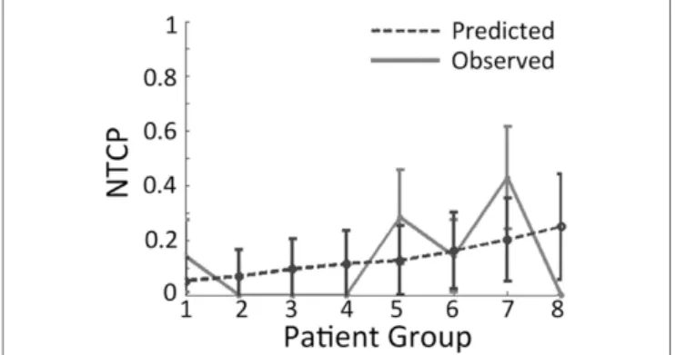
Octile Plots
Plots whereby outcomes are split into eight groups (octiles) are called octile plots (Figure 5). By considering and plotting both the predicted and observed outcomes, the plot provides a two-dimensional method to visually assess model fit. Furthermore,
FIGURE 5|Example of an octile plot demonstrating how patients are sub-divided into eight groups and then stratified according to the risk given by the model of interest.
octile plots allow the reader to gage how the overall model output varies with increasing magnitude of input parameters.
Receiver-Operating Characteristic Plot
As discussed previously, the ROC plot can provide a method for visually assessing model performance. Although the AUC param-eter derived from the ROC plot is reported more often, the ROC plot itself is also useful as it provides information on how the sensi-tivity varies with the specificity for different threshold cut-offs. In our work, we often use ROC plots alongside AUCs and correlation coefficients to gain a full understanding of how a particular model behaves under conditions of cross-validation (60).Vector Biplots
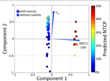
Biplots display vectors that are constructed and presented along-side PCA-derived information and patient-specific NTCP. In the context of model visualization, vector biplots provide a rough estimate of which variables are able to explain the data – this is generally accomplished in two dimensions to aid visualizing the model on paper.
PCA and Kernel-PCA
Principle component analysis is useful as a method to reduce the dimensionality of data into either two- or three-dimensions to facilitate performance visualization. The trade-off in using PCA for outcome modeling is that the relationships between inputs and outcomes are highly non-linear and, therefore, true relationships may not be adequately captured by the technique. Alternatively, the previously described Kernel-PCA technique can be employed to visualize data by improving separation between clusters. Vector biplots, two- and three-dimensional kPCA plots can indeed be used together in order to provide easy-to-interpret heat maps colorized by estimated patient-specific risk (Figure 6) (147).
FIGURE 6|Example of a color-washed vector biplot. The cardinal plane represents the vector biplot relating to the magnitude of the contribution of the variables contained within the model. The axes on which the vector biplot is shown are derived via principle component analysis (PCA). Dummy patients with toxicity were circled with empty red circles and color-washed according to NTCP values generated via the model.
CONTROVERSIES
The number of variables in a big data analysis of outcome models can accumulate quickly, especially if considering many biologi-cal factors. Several of the modeling techniques presented herein fail to take into account or mitigate the dilemma of multiple comparisons of chance correlations. Therefore, in all aspects of modeling, independent validation phases should be integrated into frameworks that aspire to produce clinically relevant results. Furthermore, although internal cross-validation techniques do provide excellent estimates of model robustness, their usefulness is limited if training samples are not retrieved from independent sources.
Radiotherapy outcomes are complex pathological manifesta-tions of the biophysical effects of ionizing radiation on the human body. Therefore, models attempting to delineate such phenom-ena should endeavor to incorporate as many different types as possible.
By definition, big data requires the ability to work with extremely large multi-dimensional datasets, which requires dedi-cated infrastructure to support access as well as high performance capabilities to facilitate efficient data exploration and modeling. Such investments require capital expenditure and training in addi-tion to the formaaddi-tion of data-sharing and privacy agreements between institutions (148).
Once meaningful analytics can readily be extracted from mul-ticenter databases, scientists and physicians are faced with the dilemma of determining how their predictive models should be used to maximize the TCP/NTCP ratio. No doubt, the afore-mentioned biological and clinical risk factors that predispose a prostate cancer patient to radiation toxicity can be quantified before therapy and used to guide initial radiation treatment plan-ning but such an approach ignores such factors as risk to long-term quality of life, intra-treatment imaging data, physiological changes during therapy, and symptoms the patient may develop during and shortly after therapy.
SOFTWARE TOOLS
Many independently verified platforms exist for data-mining and analytics exploration, several of which are listed below with brief explanations of their scope and limitations. Further details on the use and QA of such software can be found in AAPM Task Group Report #166 (149).
BIOlogical Evaluation of PLANs (BIOPLAN)
Bioplan is a user-friendly software developed in the United King-dom that allows an absorbed dose treatment plan to be converted into its likely biological effect (150). It provides a variety of tools, including DVH subtraction, and is able to calculate NTCP val-ues according to previously described LKB and binomial-based models.Computational Environment for
Radiotherapy Research
Computational environment for radiotherapy research (CERR) is an open-source computational environment that facilitates the
conversion of treatment plan data into MATLAB (151). The software allows for either retrospective or experimental treatment planning and can read-in CT data as well as associated contours. In the past, our group has used CERR in investigating both GU and GI toxicities in prostate cancer. CERR can also be used to estimate the contribution of joint-contours, such as rectal margin overlap with the PTV, to toxicities.
Dose Response Explorer System
Dose response explorer system (DREES) is an open-source data-mining tool for exploring dose–response relationships (142). Using a built in subroutine called CERR+, the program imports patient data from CERR. DREES provides a suite of tools for either NTCP or TCP modeling of outcomes without restric-tion as to the site or popularestric-tion size. The program includes a GUI interface within MATLAB in order to simplify usability. Examples of the functions contained with DREES include logis-tic regression, LKB modeling, actuarial statislogis-tics, bootstrap val-idation, Kaplan–Meier survival analysis, nomograms, boxplots, and has the functionality for interfacing with SVMs. One of the major advantages of using DREES is it that it freely distributed, as is CERR, and is consistently updated, making it flexible and adaptable.
FUTURE TRENDS
Implications of Charged Particle Therapy
The use of charged particle therapy in treating prostate cancer has become more mainstream over the past decade, mainly in the United States (152). Unfortunately, comparable outcome data from a treatment delivery technology point of view on the use of proton therapy vs. photon therapy for prostate cancer (to an even lesser extent carbon ion therapy) are not yet readily available. Unlike the mainstream adoption of RBE=1.1 for pro-ton therapy (153), the RBE debate for charged particles contin-ues, which makes outcomes comparison to photons difficult for heavier charged particles and prospective outcomes prediction impossible.Studies published using modulated proton techniques report that GI/GU late effects post-RT are either unchanged (154) or reduced (155–157). In the case of carbon ions, extensive long-term biochemical outcomes are not yet available and so does the interpretation of the efficacy of such treatments remains difficult. In terms of late radiation-induced ED, at least one study has shown no significant upregulation using protons (158).
The impact of charged particle therapy plans on outcome mod-eling is that thresholds, such as those proposed by QUANTEC, will likely need to be adjusted given the differences in dose distri-bution and biological response relative to photon-based therapy (159,160).
Advanced Methods in Machine Learning
Examples of more complex modeling techniques include the use of restricted Boltzmann machines (RBMs), which are energy-based multilayered graphical models that estimate the joint prob-ability distribution between inputs and outcomes using one or more binary stochastic hidden layers (161–163). The concept ofan RBM was first proposed by Prof. Geoffrey Hinton from the University of Toronto in 2006 as a method to efficiently train and learn a constrained version of a Boltzmann machine (164). RBMs as applied to oncology have shown promise in making accurate predictions, however, they remain relatively poorly dis-seminated techniques and their implementation to date has been limited.
Multilayered networks, such as RBM or convolutional neu-ral network, can performdeep learning in that data are passed through more than one layers of machine-learning modules that combine to form a framework capable of processing highly com-plex patterns. More specifically, deep learning strategies attempt to model high-level abstractions, such as the recognition of three-dimensional objects, in order to label and classify. This may prove extremely useful in the case of radiation-induced biological effects given the physical understanding that such phenomena manifest after cascading effects at the atomic, molecular, and then cellular levels. Previously, modeling strategies involving deep learning in the form of deep belief networks (DBNs) have been applied to data in oncology via multilayered RBMs, which are known as deep Boltzmann machines (DBMs) (165,166). Such applications are, for instance, infrequent but may become more frequent as tech-niques are disseminated and refined specifically for the purposes of radiation oncology.
CONCLUSION
Prostate cancer is one of the most commonly diagnosed cancers across the globe and radiation therapy is a primary modality in treating such cases. Prostate cancer is a heterogeneous disease at several levels (pathological, molecular/genetic, and clinical) and, despite technical improvements, there is still a significant risk of cancer recurrence after therapy. Treatment efficacy for localized prostate cancer has increased greatly in recent years; however, few efforts have been aimed at developing and testing personalized predictive metrics, namely those identified through the rapidly advancing field of big data analytics using machine learning and artificial intelligence. Such analytics would allow prostate radio-therapy regimens to be further tailored to the individual and gen-erate treatment plans that are functions of not only dose–volume metrics but also individual’s clinical risk factors and biological parameters.
Given the apparent complexity of physiological response to ionizing radiation, it is likely that systems-based approaches will play a larger role in radiotherapy outcome modeling in the future. Although regression-based techniques have yielded success in cer-tain cases, their cross-validated prediction performance appears to be generally limited, likely due to their inability to capture higher order interactions between biophysical processes.
A chief limitation in modern outcome modeling projects is the difficulty in pooling sets of data from multiple institutions. In medicine, this is principally due to privacy and security con-cerns. If, however, proper data-sharing protocols can be put in place, big data analytics may provide a significant boost to data-driven outcome models owing not only to larger datasets but also to the ability to more readily perform independent validation.
AUTHOR CONTRIBUTIONS
The initial conception of the review article was proposed by IN and the initial draft was compiled by JC. Multiple rounds of peer
editing by both JC and IN then took place until LS was contacted at the request of the editors in order to review the manuscript for clinical input. All figures were selected and compiled together by JC, LS, and IN.
REFERENCES
1. UK CR. Prostate cancer statistics. Cancer Stat (2011). Available from: http://www.cancerresearchuk.org/health-professional/cancer-statistics/ statistics-by-cancer-type/prostate-cancer#heading-Zero
2. Ferlay J, Steliarova-Foucher E, Lortet-Tieulent J, Rosso S, Coebergh JWW, Comber H, et al. Cancer incidence and mortality patterns in Europe: estimates for 40 countries in 2012.Eur J Cancer(2013) 49:1374–403. doi:10.1016/j.ejca. 2012.12.027
3. Network NCI.Treatment Routes in Prostate Cancer. Bristol, UK (2009). 4. Sriprasad S, Feneley MR, Thompson PM. History of prostate cancer treatment.
Surg Oncol(2009) 18:185–91. doi:10.1016/j.suronc.2009.07.001
5. Bauman G, Rumble RB, Chen J, Loblaw A, Warde P, Members of the IMRT Indications Expert Panel. Intensity-modulated radiotherapy in the treatment of prostate cancer.Clin Oncol (R Coll Radiol)(2012) 24:461–73. doi:10.1016/j. clon.2012.05.002
6. Musunuru HB, Loblaw A. Clinical trials of stereotactic ablative radiother-apy for prostate cancer: updates and future direction.Future Oncol(2015) 11:819–31. doi:10.2217/fon.15.14
7. De Ruysscher D, Mark Lodge M, Jones B, Brada M, Munro A, Jefferson T, et al. Charged particles in radiotherapy: a 5-year update of a systematic review.
Radiother Oncol(2012) 103:5–7. doi:10.1016/j.radonc.2012.01.003 8. Hummel S, Simpson EL, Hemingway P, Stevenson MD, Rees A.
Intensity-modulated radiotherapy for the treatment of prostate cancer: a systematic review and economic evaluation.Health Technol Assess(2010) 14:1–108,iii–iv. doi:10.3310/hta14470
9. Milano MT, Constine LS, Okunieff P. Normal tissue tolerance dose metrics for radiation therapy of major organs.Semin Radiat Oncol(2007) 17:131–40. doi:10.1016/j.semradonc.2006.11.009
10. Mundt A, Boeske JC.Intensity Modulated Radiation Therapy: A Clinical Per-spective. Tokyo (2005). p. 151–2.
11. Marks LB, Yorke ED, Jackson A, Ten Haken RK, Constine LS, Eisbruch A, et al. Use of normal tissue complication probability models in the clinic.Int J Radiat Oncol Biol Phys(2010) 76:S10–9. doi:10.1016/j.ijrobp.2009.07.1754 12. Bentzen SM, Parliament M, Deasy JO, Dicker A, Curran WJ, Williams JP,
et al. Biomarkers and surrogate endpoints for normal-tissue effects of radiation therapy: the importance of dose-volume effects.Int J Radiat Oncol Biol Phys
(2010) 76:S145–50. doi:10.1016/j.ijrobp.2009.08.076
13. Deasy JO, Mayo CS, Orton CG. Treatment planning evaluation and opti-mization should be biologically and not dose/volume based.Med Phys(2015) 42:2753–6. doi:10.1118/1.4916670
14. El Naqa I, Bradley J, Blanco AI, Lindsay PE, Vicic M, Hope A, et al. Multivari-able modeling of radiotherapy outcomes, including dose–volume and clinical factors.Int J Radiat Oncol Biol Phys(2006) 64:1275–86. doi:10.1016/j.ijrobp. 2005.11.022
15. Lambin P, Rios-Velazquez E, Leijenaar R, Carvalho S, van Stiphout RGPM, Granton P, et al. Radiomics: extracting more information from medical images using advanced feature analysis.Eur J Cancer(2012) 48:441–6. doi:10.1016/j. ejca.2011.11.036
16. Rosenstein BS, West CM, Bentzen SM, Alsner J, Andreassen CN, Azria D, et al. Radiogenomics: radiobiology enters the era of big data and team science.Int J Radiat Oncol Biol Phys(2014) 89:709–13. doi:10.1016/j.ijrobp. 2014.03.009
17. Keetch DW, Humphrey PA, Smith DS, Stahl D, Catalona WJ. Clinical and pathological features of hereditary prostate cancer.J Urol(1996) 155:1841–3. doi:10.1016/S0022-5347(01)66024-5
18. Epstein JI, Walsh PC, Carmichael M, Brendler CB. Pathologic and clinical findings to predict tumor extent of nonpalpable (stage T1c) prostate cancer.
JAMA(1994) 271:368–74. doi:10.1001/jama.271.5.368
19. Heppner GH, Miller BE. Tumor heterogeneity: biological implications and therapeutic consequences.Cancer Metastasis Rev(1983) 2:5–23. doi:10.1007/ BF00046903
20. Mackinnon AC, Yan BC, Joseph LJ, et al. Molecular biology underlying the clinical heterogeneity of prostate cancer: an update.Arch Pathol Lab Med
(2009) 133:1033–40. doi:10.1043/1543-2165-133.7.1033
21. Taylor BS, Schultz N, Hieronymus H, Gopalan A, Xiao Y, Carver BS, et al. Integrative genomic profiling of human prostate cancer.Cancer Cell(2010) 18:11–22. doi:10.1016/j.ccr.2010.05.026
22. Kirkpatrick JP, Meyer JJ, Marks LB. The linear-quadratic model is inappropri-ate to model high dose per fraction effects in radiosurgery.Semin Radiat Oncol
(2008) 18:240–3. doi:10.1016/j.semradonc.2008.04.005
23. Jones B, Dale RG. Mathematical models of tumour and normal tissue response.
Acta Oncol(1999) 38:883–93. doi:10.1080/028418699432572
24. Brenner DJ, Hall EJ. Fractionation and protraction for radiotherapy of prostate carcinoma.Int J Radiat Oncol Biol Phys(1999) 43:1095–101. doi:10.1016/ S0360-3016(98)00438-6
25. Fowler J, Chappell R, Ritter M. Is α/β for prostate tumors really low?
Int J Radiat Oncol Biol Phys(2001) 50:1021–31. doi:10.1016/S0360-3016(01)
01607-8
26. Fowler JF. The radiobiology of prostate cancer including new aspects of fractionated radiotherapy. Acta Oncol (2005) 44:265–76. doi:10.1080/ 02841860410002824
27. Dasu A. Is theα/βvalue for prostate tumours low enough to be safely used in clinical trials?Clin Oncol(2007) 19:289–301. doi:10.1016/j.clon.2007.02.007 28. Kupelian PA, Thakkar VV, Khuntia D, Reddy CA, Klein EA, Mahadevan
A. Hypofractionated intensity-modulated radiotherapy (70 Gy at 2.5 Gy per fraction) for localized prostate cancer: long-term outcomes.Int J Radiat Oncol Biol Phys(2005) 63:1463–8. doi:10.1016/j.ijrobp.2005.05.054
29. Arcangeli G, Saracino B, Gomellini S, Petrongari MG, Arcangeli S, Sentinelli S, et al. A prospective phase III randomized trial of hypofractionation versus conventional fractionation in patients with high-risk prostate cancer.Int J Radiat Oncol Biol Phys(2010) 78:11–8. doi:10.1016/j.ijrobp.2009.07.1691 30. King CR, Brooks JD, Gill H, Pawlicki T, Cotrutz C, Presti JC. Stereotactic
body radiotherapy for localized prostate cancer: interim results of a prospective phase II clinical trial.Int J Radiat Oncol Biol Phys(2009) 73:1043–8. doi:10. 1016/j.ijrobp.2008.05.059
31. Vogelius IR, Bentzen SM. Meta-analysis of the alpha/beta ratio for prostate cancer in the presence of an overall time factor: bad news, good news, or no news?Int J Radiat Oncol Biol Phys(2013) 85:89–94. doi:10.1016/j.ijrobp.2012. 03.004
32. Dörr W, Hendry JH. Consequential late effects in normal tissues.Radiother
Oncol(2001) 61:223–31. doi:10.1016/S0167-8140(01)00429-7
33. Pinkawa M, Holy R, Piroth MD, Fischedick K, Schaar S, Székely-Orbán D, et al. Consequential late effects after radiotherapy for prostate cancer – a prospective longitudinal quality of life study.Radiat Oncol(2010) 5:27. doi:10.1186/1748-717X-5-27
34. Pinkawa M, Ribbing C, Djukic V, Klotz J, Holy R, Eble MJ. Early hemato-logic changes during prostate cancer radiotherapy predictive for late urinary and bowel toxicity.Strahlentherapie Und Onkol Organ Der Dtsch Röntgenge-sellschaft(2015) 191:771–7. doi:10.1007/s00066-015-0841-3
35. Drodge CS, Boychak O, Patel S, Usmani N, Amanie J, Parliament MB, et al. Acute toxicity of hypofractionated intensity-modulated radiotherapy for prostate cancer.Curr Oncol(2015) 22:e76–84. doi:10.3747/co.22.2247 36. Zietman AL. The Titanic and the iceberg: prostate proton therapy and
health care economics.J Clin Oncol(2007) 25:3565–6. doi:10.1200/JCO.2007. 11.9768
37. Yu JB, Soulos PR, Herrin J, Cramer LD, Potosky AL, Roberts KB, et al. Proton versus intensity-modulated radiotherapy for prostate cancer: patterns of care and early toxicity.J Natl Cancer Inst(2013) 105(1):25–32. doi:10.1093/jnci/ djs463
38. Fang P, Mick R, Deville C, Both S, Bekelman JE, Christodouleas JP, et al. A case-matched study of toxicity outcomes after proton therapy and intensity-modulated radiation therapy for prostate cancer.Cancer(2015) 121:1118–27. doi:10.1002/cncr.29148