hpcNMF: A high-performance toolbox for non-negative matrix factorization

Collection of Biostatistics Research Archive

COBRA Preprint Series

Year  Paper

hpcNMF: A high-performance toolbox for

non-negative matrix factorization

Karthik Devarajan

Guoli Wang

∗_{Fox Chase Cancer Center, [email protected]}

†_{3M Healthcare, [email protected]}

This working paper is hosted by The Berkeley Electronic Press (bepress) and may not be commer-cially reproduced without the permission of the copyright holder.

http://biostats.bepress.com/cobra/art115

hpcNMF: A high-performance toolbox for

non-negative matrix factorization

Karthik Devarajan and Guoli Wang

Abstract

Non-negative matrix factorization (NMF) is a widely used machine learning algo-rithm for dimension reduction of large-scale data. It has found successful appli-cations in a variety of fields such as computational biology, neuroscience, natural language processing, information retrieval, image processing and speech recog-nition. In bioinformatics, for example, it has been used to extract patterns and profiles from genomic and text-mining data as well as in protein sequence and structure analysis. While the scientific performance of NMF is very promising in dealing with high dimensional data sets and complex data structures, its computa-tional cost is high and sometimes could be critical for delivering analysis results in a timely manner. In this paper, we describe a high-performance C++ tool-box for NMF, called hpcNMF, that is designed for use on desktop computers and distributed computer clusters. Algorithms based on different statistical models and cost functions as well as various metrics for model selection and evaluating goodness-of-fit are implemented in the toolbox. hpcNMF is platform indepen-dent and does not require the use of any special libraries. It is compatible with Windows, Linux and Mac operating systems; and message-passing interface is required for hpcNMF to be deployed on computer clusters to leverage the power of parallelized computing. We illustrate the utility of this toolbox using several real examples encompassing a broad range of applications.

hpcNMF: A high-performance toolbox for

non-negative matrix factorization

Karthik Devarajan

∗

a_{Department of Biostatistics & Bioinformatics, Fox Chase Cancer Center,}

Temple University Health System, Philadelphia, PA

Guoli Wang

b_{3M Healthcare, Bethesda, MD}

Abstract

Non-negative matrix factorization (NMF) is a widely used machine learning algo-rithm for dimension reduction of large-scale data. It has found successful appli-cations in a variety of fields such as computational biology, neuroscience, natural language processing, information retrieval, image processing and speech recognition. In bioinformatics, for example, it has been used to extract patterns and profiles from genomic and text-mining data as well as in protein sequence and structure analysis. While the scientific performance of NMF is very promising in dealing with high dimensional data sets and complex data structures, its computational cost is high and sometimes could be critical for delivering analysis results in a timely manner. In this paper, we describe a high-performance C++ toolbox for NMF, calledhpcNMF, that is designed for use on desktop computers and distributed computer clusters. Algorithms based on different statistical models and cost functions as well as var-ious metrics for model selection and evaluating goodness-of-fit are implemented in the toolbox.hpcNMF is platform independent and does not require the use of any special libraries. It is compatible with Windows, Linux and Mac operating systems; and message-passing interface is required for hpcNMFto be deployed on computer clusters to leverage the power of parallelized computing. We illustrate the utility of this toolbox using several real examples encompassing a broad range of applications.

Key words: non-negative matrix factorization, high-performance computing, message-passing interface, high dimensional data, bioinformatics, text mining

∗ _{Corresponding author.}

Email addresses: [email protected] (Karthik Devarajan),

1 Background

NMF is a powerful approach for factoring a high dimensional nonnegative matrixV into the

product of two nonnegative matrices W and H. In the context of a p×n gene expression

matrix V consisting of observations on p genes from n samples, each column of W defines

a metagene and each column of H represents the metagene expression pattern of the

corre-sponding sample. Since its introduction by Lee and Seung (1999,2001), NMF has been widely used in a variety of fields such as computational biology, neuroscience, natural language pro-cessing, information retrieval, image processing and speech recognition. In bioinformatics, it has been primarily used for analyzing and interpreting large-scale biological data such as those arising from studies of gene expression, protein sequence and structure and biomedi-cal text (see Devarajan (2008) for a review of this method). Relative to other unsupervised clustering algorithms commonly used for analyzing such large-scale data, NMF has been shown to have superior performance in terms of homogeneity of clustering and prediction of gene function (Kim & Tidor, 2003; Brunet et al., 2004; Devarajan et al., 2005, 2008; Wang et al., 2005; Chagoyen et al., 2006; Okun & Priisalu, 2006; Gajoux & Seoghie, 2012). The major advantage of the NMF algorithm over other matrix factorization methods is the non-negativity constraint imposed on the model. The non-negativity constraint provides a parts-based representation of the original data set, resulting in easier interpretation and un-derstanding of the biological context. Another important advantage of NMF is its relative ease of implementation due to multiplicative or gradient-based update rules.

Over the last several years, many variants have been proposed to improve the performance over the standard NMF algorithm. Examples include Cheung & Tresch (2005), Dhillon & Sra (2005), Pascual-Montano et al. (2006), Berry et al. (2007), Cichocki et al. (2006, 2008, 2009),

Kompass (2007), Devarajan & Ebrahimi (2005, 2006, 2008, 2011), F´evotte & Idier (2011),

Gillis & Glineur (2010, 2012), Zhou et al. (2012), Devarajan & Cheung (2014), Devarajan et al. (2015) and references cited therein. Although some efficient implementations exist, many of the improvements come with the price of increasing computational complexity. From a software implementation point of view, these variants and possible future variants could be easily implemented under object oriented design because the application framework is the same, and only the update rules need to change accordingly. It is feasible to parallelize NMF simulations on distributed computer clusters. At the time of this writing, we are not aware of any publicly available open source implementations with high-performance computing (HPC) compatibility.

2 Methods

Gene expression data from a set of experiments is presented as a matrix in which columns correspond to expression levels of genes, rows to samples (which may represent distinct tissues, experiments or time points) and each entry to the expression level of a given gene in

a given sample. In gene expression studies, the number of genespis typically in the thousands;

the number of samples,n, is typically less than one hundred and the expression matrix V is

of size p×n, whose columns contain the expression levels of pgenes in n samples. Our goal

is to find a small number of metagenes, each defined as a nonnegative linear combination

of the p genes. This is accomplished via a decomposition of the expression matrix V into

two matrices with nonnegative entries such that Vp×n ∼ Wp×kHk×n. Each column of W

defines a metagene and each column of H represents the metagene expression pattern of the

corresponding sample. The rankk of the factorization is chosen so that (n+p)k < np. Here,

the entry wia in the matrix W is the coefficient of gene i in metagene a and the entry haj

in the matrix H is the expression level of metagenea in gene j. There is a dual view of the

decomposition given by V′ ∼ H′W′ based on the transpose of V that defines metasamples

rather than metagenes. Devarajan (2008) discussed the numerous applications of NMF in computational biology.

Throughout this article, the term gene expression data has a broader connotation and is used to refer to data obtained from a variety of technologies such as microarrays, single nucleotide polymorphism arrays, methylation arrays, allele-specific expression, microRNA

and next-generation sequencing studies.1

Given the input matrix V and factorization rank k, the goal is to find nonnegative matrices

W and H such thatV ≈W H. This can be represented by the bi-linear model,

V =W H+ϵ, (2.1)

whereϵ represents the noise distribution and bothW and H are unknown. An approximate

factorization for V is obtained by defining a cost function that measures the divergence

between V and W H for a given rank k. Various cost functions have been proposed in the

literature based on an assumed or empirically determined noise distribution such as the Gaussian, Poisson, gamma or the inverse Gaussian model. These cost functions are typically

derived from Kullback-Leibler (KL) divergence, its dual or a generalization for a particular

model or class of models. One example is the Euclidean distance (ED),

ED(V||W H) = KL(V||W H) = 1

2σ2

∑ i,j

(Vij −(W H)ij)2, (2.2)

which is based on the Gaussian likelihood and was proposed by Lee & Seung (2001).

Al-though not generally recognized, the quantity in (2.2) can be derived as the KL divergence

between two Gaussian random variables with meansµ1 =Vij andµ2 = (W H)ij and common

dispersion (variance) parameterσ2 (Devarajan et al., 2006; 2011; 2015). Lee & Seung (2001)

also proposed a cost function based on the Poisson likelihood and referred to this quantity as

“KL” divergence. However, the termKLdivergence is used in a broader context throughout

this presentation and is based on the divergence between V and W H for a given statistical model specified by one of the noise distributions above. The goal is to minimize the cost

function, such as KL(V||W H) above, with respect to W and H, subject to the constraints

W, H ≥ 0. Non-negativity requirements on V and random starting values for W and H

combined with multiplicative updates ensure non-negativity of the final converged solution

for W and H. However, other types of updates such as those based on the gradient are also

possible (Cheung & Tresch, 2005; Cichocki et al., 2009; Zhou et al., 2012;).

2.1 The Gaussian model

The Gaussian model-based algorithm is perhaps the most commonly used version of NMF.

Ifϵin (2.1) is a Gaussian random variable, thenKLdivergence between V andW H for this

model is given by (2.2) above. For this model, update rules for H and W are given by

H_ajt+1 =H_ajt ( _∑ iVijWia ∑ iWia( ∑ bWibHbjt) ) (2.3) and W_iat+1 =W_iat ( ∑ jHajVij ∑ j( ∑ bWibtHbj)Haj ) .

2.2 The Poisson model

In the context of gene expression and text mining data, the generalized approach of Devarajan et al. (2005,2008,2015) is based on Renyi divergence that is related to the Poisson likelihood

of generatingV fromW H. If ϵin (2.1) is a Poisson random variable, then Renyi divergence

between V and W H is given by

Dα(V||W H) = 1 α−1 ∑ i,j [ V_ijα(W H)1_ij−α−αVij −(1−α)(W H)ij ] . (2.4)

From (2.4) above, we see that Renyi divergence is indexed by the parameterα,(α ̸= 1) and

it represents a continuum of distance measures simply based on the choice of this parameter. Several well-known divergence measures are members of this family. Some examples include

KL divergence (α → 1), Pearson’s chi-squared statistic (α = 2) and the symmetric

Bhat-tacharya distance (α = 0.5). For details, the interested reader is referred to Devarajan et al.

Minimizing the divergenceDα(V||W H) with respect toW and H, subject to the constraints

W, H ≥0, results in multiplicative update rules given by

H_ajt+1=H_ajt       ∑ i ( Vij ∑ bWibHbjt )α Wia ∑ iWia       1/α and W_iat+1=W_iat       ∑ j ( Vij ∑ bWibtHbj )α Haj ∑ jHaj       1/α . (2.5)

See Devarajan et al. (2015) for a derivation of these update rules. Independently, several generalized divergence measures for NMF have been proposed in the machine learning lit-erature. These include Dhillon & Sra (2005), Cichocki et al. (2006, 2008, 2009, 2011) and Kompass (2007). Many of these measures are related to Renyi divergence via scale or power transformations.

2.3 The Gamma model

NMF algorithms based on the gamma model for handling signal dependent noise have also been proposed in the literature and successfully applied in many areas of statistical signal

processing (Cheung & Tresch, 2005; Cichocki et al., 2006; F´evotte & Idier, 2011; Devarajan

& Cheung, 2014). If ϵ in (2.1) is a gamma random variable, then KL divergence for the

gamma model can be expressed in terms of V and W H as

KL(V||W H) = γ∑ i,j { −log ( Vij (W H)_ij ) + Vij (W H)_ij −1 } , (2.6)

whereγ >0 is the dispersion parameter. Minimizing this divergence with respect to W and

H, subject to the constraints W, H ≥0, results in multiplicative update rules given by

H_ajt+1=H_ajt       ∑ i Vij (∑_bWibHbjt ) 2Wia ∑ i ( 1 ∑ bWibHbjt ) Wia       (2.7)

and W_iat+1=W_iat       ∑ j Vij (∑_bWt ibHbj)2 Haj ∑ j ( 1 ∑ bWibtHbj ) Haj      .

A heuristic derivation of these update rules is provided in Cheung & Tresch (2005) and

Ci-chocki et al. (2006). The generalizedβ-divergence proposed by Cichocki et al. (2006) embeds

the so called Itakura-Saito (IS) divergence which can be obtained as theKL divergence

be-tween two exponential random variables with different means (obtained by setting γ = 1 in

(2.6)). Furthermore, IS divergence can be shown to be equivalent to the KL divergence

be-tween two gamma random variables with different scale parameters and common dispersion

(shape) parameter γ.

Recently Devarajan & Cheung (2014) outlined NMF algorithms for the gamma model based

on dual KLdivergence and the symmetric J-divergence. For a given model, dualKL

diver-gence (denoted asKLd_{) is obtained by reversing the roles ofV and W H while J-divergence}

(denoted as J) is obtained as the sum of KL and dual KL divergences. Using (2.6), dual

KL divergence the gamma model can be written as

KLd(W H||V) = γ∑ i,j { log ( Vij (W H)_ij ) +(W H)ij Vij −1 } . (2.8)

The corresponding update rules for H and W are

H_ajt+1=H_ajt       ∑ i ( 1 ∑ bWibHbjt ) Wia ∑ i ( Wia Vij )       (2.9) and W_iat+1=W_iat       ∑ j ( 1 ∑ bWibtHbj ) Haj ∑ j ( Haj Vij )      .

Similarly, J divergence for the gamma family is obtained by summing the right hand sides

J(V||W H) =γ∑ i,j    (Vij−(W H)ij) 2 Vij(W H)ij   . (2.10)

The corresponding update rules for H and W are

H_ajt+1=H_ajt        ∑ i ( Vij ∑ bWibHbjt )2( Wia Vij ) ∑ i ( Wia Vij )        1/2 (2.11) and W_iat+1=W_iat        ∑ j ( Vij ∑ bWibtHbj )2( Haj Vij ) ∑ j ( Haj Vij )        1/2 .

A derivation of the update rules in (2.9) and (2.11) is provided in Devarajan & Cheung (2014).

2.4 The Inverse Gaussian Model

Dual KL divergence for the inverse Gaussian family is given by

KLd(W H||V) = λ 2 ∑ i,j {Vij −(W H)_ij}2 V2 ij(W H)_ij , (2.12)

where λ >0 is the dispersion parameter. The corresponding update rules forH and W are

H_ajt+1=H_ajt        ∑ i ( Vij ∑ bWibHbjt )2( Wia Vij2 ) ∑ i ( Wia Vij2 )        1/2 (2.13) and

W_iat+1=W_iat        ∑ j ( Vij ∑ bWibtHbj )2( Haj Vij2 ) ∑ j ( Haj Vij2 )        1/2 .

This algorithm was also proposed in Devarajan & Cheung (2014) where a derivation of the update rules is provided.

Remark 1 (Dispersion parameter) In the above formulations, the dispersion

parame-ters σ, γ and λ do not play any role in the minimization of the objective function or in the

derivation of update rules for W and H. Hence, without loss of generality it is assumed that

2σ2 =γ = λ₂ = 1 in eqns. (2.2),(2.6),(2.8),(2.10) and (2.12).

2.5 Convergence of the Algorithm

A maximum of 2000 iterations are utilized by default for a given run of the algorithm. For

each run, convergence is determined based on a pre-specified upper boundϵ0 for the absolute

difference between consecutive iterates. The default setting automatically checks for

conver-gence based on this criterion.hpcNMF counts the number of iterations until convergence for

each run and computes the mean number of iterations required for convergence, mean

recon-struction error, mean fraction of converged runs and mean ϵ0 across N pre-specified runs.

There is an option available to override the test for convergence and to let the algorithm run

for a pre-specified number of iterations. The base seed for random initializations for W and

H is set to 12458698 but can be changed if desired.

3 Model selection

In NMF, selecting the optimal dimensionality of the factorization or the number of clusters

(k) is an important consideration. In this section, model selection for a given data set with

unknown classes for the samples is described. Given random initial starting values for W

and H, the update rules for a chosen model guarantee convergence of the algorithm to a

local minimum. Random initial conditions in NMF enable quantitative evaluation of the consistency of the performance of the algorithm based on multiple runs. The algorithm

groups the samples intok clusters, wherek is the pre-specified rank of the factorization. For

each run of the NMF algorithm, the cluster membership for each sample is determined based on the highest metagene expression profile, i.e., given by the highest entry in each column

of H. There is an option available in hpcNMF to cluster based on rows of W which may

be necessary in certain applications (see examples in §6.1.2 and §6.3.1). In our studies, the

50-200 runs were sufficient to provide stability to the clustering (Devarajan et al., 2008, 2015; Brunet et al., 2004).

3.1 Consensus Clustering

In order to assess whether a given rank k provides a biologically meaningful decomposition

of the data, the information obtained from multiple runs of the NMF algorithm can be combined via consensus clustering (Brunet et al., 2004; Monti et al., 2003; Devarajan, 2008). This approach provides a quantitative evaluation of the robustness of the factorization.

Suppose we are applying NMF to cluster n samples. For a given rank k factorization, each

run of the algorithm results in a connectivity matrix C with an entry of 1 if samples iand j

cluster together and 0 otherwise, where i, j = 1, .., p. The average connectivity matrix over,

say,N runs is the consensus matrix ¯C. Hierarchical clustering (HC) (using average linkage) is

then applied to ¯C to visualize the clusters via a heat map of the re-ordered consensus matrix.

Final sample assignments to each cluster are based on the re-ordered consensus matrix.

hpcNMF implements a variety of metrics for model selection and quantifying clustering

ho-mogeneity/accuracy. These include the cophenetic correlation coefficientρ, the overall cluster

consensusκ, normalized mutual information (NMI) and the adjusted Rand index (ARI). The

cophenetic correlation coefficientρ(0≤ρ≤1) is defined as the Pearson correlation between

1−C¯ and the distance induced by HC using average linkage (Brunet et al., 2004). hpcNMF

also implements an equivalent version ofρbased on the Spearman rank correlation, denoted

as ˜ρ, that is robust to distributional assumptions on the computed distances. Another useful

measure for evaluating cluster homogeneity is thecluster consensus (κl). For a given cluster

l,l = 1, ..., k, it is defined as the mean consensus index between all pairs of samples belonging

to the same cluster and is given by

κl = 1 nl(nl−1)/2 ∑ i,j∈Il i<j ¯ C_ijl , l= 1, ..., k (3.14)

whereIl={a:ea∈l}is the set of indices of samples belonging to clusterl,nl is the number

of samples in cluster l, ¯Cl _{is the consensus matrix of thel}th _{cluster, and 0< κ}

l <1 for each

l. Based on this, the overall cluster consensus (κ) is defined as the mean consensus index

between all pairs of samples belonging to the same cluster, averaged across the k clusters. It

is given by κ= ∑_k l=1 ∑ i,j∈Il i<j ¯ Cl ij ∑_k l=1nl(nl−1)/2 (3.15)

where 0< κ <1. Given a consensus matrix ¯C, the total point scatterdenoted byτ is defined as τ = k ∑ l=1 ∑ i,j 1−C¯_ijl

where τ > 0. τ is independent of cluster assignment and is a constant for a given data set.

Theoverall within-cluster point scatter, denoted byω, measures the degree to which samples

assigned to the same cluster are close to one another, averaged across the K clusters and

expressed as a fraction of τ. It is defined as

ω = ∑_k l=1 ∑ i,j∈Il i<j 1−C¯_ijl τ ·∑k_l=1nl(nl−1)/2 (3.16)

where 0 < ω < 1. A value close to zero for ω indicates tight clustering of samples. From

(3.15) and (3.16), it is straightforward to see that ω = (1−_τκ), i.e., higher the overall cluster consensus, smaller the within-cluster point scatter. Even though HC has been used for final

sample assignments based on the re-ordered consensus matrix for each pre-specified rank k

and α, other methods such as K-medoids (Hastie et al, 2001) could also be used for this

task. Regardless of the approach, the identification of homogeneous clusters using κ would

remain the same. The use of κ is flexible enough to accommodate the use of practically any

method for final sample assignments based on the re-ordered consensus matrix. On the other

hand, it should be noted that the use of ρ is restricted to the use of only HC (sinceρ is the

correlation between 1−C¯ and the distance induced by HC using average linkage). Moreover,

the problems associated with ρ have been well documented in the literature (Hastie et al.,

2001; Holgersson, 1978). In our studies we observed that the range of values of κ was much

wider than that of ρ across values of α for a fixed rank k; as well as across various ranks k

for a chosen value ofα. Overall, we foundκto be a very useful alternative toρin delineating

clusters. This is exemplified by the numerical results in§6 using real-life gene expression and

text mining data.

Measures based on cluster consensus also provide a probabilistic interpretation of cluster

membership and of associations between pairs of samples. While κ provides an overall

mea-sure of homogeneity across all clusters for a given rankk, the relative homogeneity of the lth

sub-cluster can be evaluated usingκl, the cluster-specific consensus wherel = 1, ..., k.κl can

be interpreted as the probability that two randomly selected samples from thelth _{cluster are}

clustered together. It enables the identification of sub-clusters showing poor homogeneity. If the true class labels were known and one was interested in evaluating the clustering

accuracy of the NMF algorithm for a range of α values, measures such as NMI, ARI and

the misclassification rate (M C, ν) could be used. For final cluster label assignments based

N M I= ∑ i,jnijlog ( n·nij ninj ) √(_∑ inilog ni n ) (_∑ jnjlog nj n )

where ni is the number of items in class i, nj is the number of items in cluster j, nij is

the number of items in class i and cluster j and n is the total number of items (Strehl &

Ghosh, 2002). ARI is another commonly used measure to quantify the agreement between

the true class labelsX and the assigned cluster labelsY. It is defined as the fraction of pairs

of samples that are both in the same class and same cluster or that are both in a different

class and different cluster, normalized to fall in the [0,1] range. For details on this measure,

the interested reader is referred to Monti et al. (2003) and references cited therein.

3.1.1 Misclassification Rate

The misclassification rate is the fraction of samples classified incorrectly based on final

as-signments using the re-ordered consensus matrix, and this is denoted byM C. An alternative

measure, denoted by ν, is the fraction of samples that are classified incorrectly by the

al-gorithm across all clusters, averaged across all runs of the alal-gorithm. M C and ν can be

calculated only if the true number of classes k=K is known. If the pre-specified rank of the

factorization k were equal to the known number of classes K, then ν would provide us with

an overall measure of agreement for the clustering. Suppose the true number of classes K

and the cluster membership of each sample are known, andnl is the true number of samples

in cluster l, l= 1, ..., K. Then ν is given by

ν = m

N ·∑K_l=1nl(nl−1)/2

(3.17)

wherenl is the total number of samples in clusterl,N is the number of runs of the algorithm

and m is the total number of misclassified samples across the K clusters and N runs of

the algorithm. The quantity 1−ν is analogous to κ; however, the former is based on the

known true number of classes K while the latter can be computed for each rank k used in

the factorization. hpcNMF implements both these measures. Depending on the number of

samples in the data set, MC based on the re-ordered consensus matrix may be granular. In

such cases,ν based on the averaged across all N runs of the NMF algorithm may provide a

more useful, less granular estimate. However, it is possible to get a different interpretation of the results depending on the data and the measure used.

It is important to note that unlike the misclassification rate, quantities such as ρ, κ, N M I

andARI can be computed even if the true number of classes K is not known. In addition to

ρ and κ, NMI and ARI can thus be used to quantify cluster homogeneity for the purpose of

model selection. The range of each measure is [0,1] where the two extreme values correspond

the information acrossN runs of the NMF algorithm and thus provide a robust quantification of the stability and sensitivity of the clustering to random initial conditions.

3.2 Proportion of Explained Variation

For a particular NMF algorithm, the proportion of explained variation (R2) for a pre-specified

rankk is a measure of the goodness-of-fit and is computed as follows. The mean

reconstruc-tion error D(V||W H), for a given model and rank k, is the estimated divergence (based

on KL, KLd or J) between V and W H averaged across N runs. Then the proportion of

explained variation for rankk can be expressed as

R2 = 1− D(V||W H)

D(V||V) . (3.18)

where D(V||V) represent the divergence between V and V where V is the grand mean of

the entries of V. Note that the calculation of D(V||V) involves replacing each entry of the

reconstructed matrix W H by the mean of all entries of the input matrix V, i.e., in the

absence of the model V ∼ W H, the best approximation of (W H)_ij is simply the average

V. For details, the interested reader is referred to see Cameron & Windmeijer (1997) and

Devarajan & Cheung (2014). For the Gaussian model, this quantity is given by

R2 = 1−      ED(V||W H) ∑ i,j ( Vij −V )2      (3.19)

where ED(V||W H) is the mean reconstruction error calculated using eqn. (2.2). A closer

look at the right hand side of eqn. (3.19) reveals that it is simply 1− RSS

SST where RSS is

the residual sum of squares and SST is the total sum of squares. A similar interpretation

holds for other algorithms. For the Poisson model, R2 is given by

R2 = 1−            Dα(V||W H) 1 α(α−1) ∑ i,j [ V_ijα(V)1−α−αVij −(1−α)V ]            (3.20)

where Dα(V||W H) is the mean reconstruction error calculated using eqn. (2.4). A table of

expressions forR2 _{for several algorithms described here is presented in Devarajan & Cheung}

(2014).hpcNMF computes R2 _{for each rank in the pre-specified range for each implemented}

3.3 Sparseness

It is well known that sparseness is a very useful feature to possess in any dimension reduction

method. The metagenes (columns of W) and the metagene expression profiles (rows of H)

in NMF are known to be typically inherently sparse even without the imposition of explicit sparseness constraints (Lee & Seung, 1999; Devarajan et al., 2015). The sparseness of a

non-negative vector x of lengthn, denoted byψ(x), is given by (Hoyer, 2004)

ψ(x) = √ n− ( ∑ ixi) √∑ ix2i √ n−1 .

This measures evaluates to zero if and only if all elements of xare equal and is unity if and

only ifxcontains a single non-zero element, and thus interpolates between the two extremes.

hpcNMFcomputes the mean sparseness of the columns and rows of the factored matrices W

and H, respectively, across N runs of the algorithm.

4 Implementation of the NMF Algorithm

4.1 Existing Software

Some NMF algorithms have been implemented in software such as Matlab (MathWorks, Natick, MA) and the R statistical language and environment (www.r-project.org). One ex-ample is the commonly used MATLAB code available from the MIT/Broad Institute website (http://www.broadinstitute.org/mpr/publications/projects/NMF/nmf.m). Available R

pack-ages in the Comprehensive R Archive Network includeNMF(Gajoux & Seoghie, 2010, 2014)

and NMFN (Liu, 2012); however, these packages and the Matlab code implement only the

standard NMF algorithms based on Gaussian and Poisson models. Recently, we created the

R package gnmf stemming from the C++ implementation described in this paper (Maisog

et al., 2014). The current version of this package, gnmf v0.7, is available at

http://cran.r-project.org/web/packages/gnmf/. It extends the basic functionality for NMF beyond the standard algorithms by incorporating Renyi divergence based on the Poisson likelihood.

Other features of hpcNMF described in this paper are currently under development in this

R package and will be available in a future version. bioNMF is a publicly available, stand

alone package for NMF that implements some basic algorithms as well visualization tools (Pascual-Montano et al., 2006). Since both Matlab and R have scalability issues either

re-lated to licensing or computational efficiency, we simultaneously developed hpcNMF using

C++ combined with different parallelization protocols. The current version of hpcNMF for

4.2 Parallelization

For any given value of the parameter α in Renyi divergence, the algorithm groups the genes

intokclusters, where k is the pre-specified rank of the factorization. This procedure requires

evaluation of various choices of α for a fixed k, each based on N runs, by computing the

corresponding values of each consensus measure (such as ρ,κ etc. described earlier). For a

typical large-scale data set, the implementation of the steps in this evaluation procedure for

each combination of (k, α) can be computationally very intensive. Even in the absence of

the parameter α such as in the Poisson, Gaussian and gamma models, the computational

cost can be expensive depending on the the size of the dataset, rank k and number of runs

N. However, these steps can be repeated for each run of the algorithm independently and

simultaneously, and the information from these runs can be combined via the consensus clustering algorithm.

The most basic implementation in hpcNMF treats every single run as a computing unit.

Since there is no information exchange between different computing units, a trivial yet very efficient parallelization protocol is to distribute computing units to various computing nodes

and cores, and then run collective calls once they are completed. Two implementations of

hpc-NMFhave been created aimed at different computer architectures: A comprehensive parallel

implementation based on message-passing interface (MPI) for distributed memory clusters (http://www-unix.mcs.anl.gov/mpi/mpich2/) and a multi-threaded version for multi-core shared memory desktops or servers. The MPI version can be beneficial if a moderate or large computer cluster is accessible. It may have a noticeable overhead dependent on network la-tency, but its advantage over multi-threaded implementation is less demanding in terms of memory requirement. Due to the nature of NMF simulations (most of the computations are independent runs based on different seeds and different ranks as described above), the MPI implementation is decoupled as much as possible, so overhead is not a significant issue. An integrated toolbox with a graphical user interface that communicates between a Windows desktop and the HPC cluster using MPI compatible software on computer clusters is also available.

4.3 C++ Core Component

The core component of hpcNMF is written in gcc compatible C++. Depending on whether

MPI is enabled, it can be compiled as an MPI capable HPC application running on computer clusters, or as a stand alone desktop executable. The multi-threaded version can be utilized on desktop computers with multi-core processors.

4.4 Web server and web interface

In addition to the C++ core component,hpcNMF also implements an apache web server to

let users run NMF smoothly from a web browser. The apache web server is written in php.

It takes user inputs, verifies and validates input data and parameters, manages intermediate files, runs NMF simulations according to user requests, updates the job status, and provides visualization of results. The visualization is powered by gnuplot, a freely distributed soft-ware. All parameters and settings are accessible from the web browser. Default values are provided for the quick launcher. As of now, this web-interface is operational only internally

at Fox Chase Cancer Center and is not part of the current version of hpcNMFaccessible via

http://devarajan.fccc.edu.

5 Results and discussion

5.1 Input data validation and default parameters setting

The first step in the process of using hpcNMF involves uploading the input data matrix V.

The input file should be tab delimited, and the rows and columns can be labeled, optionally, by including column labels as the first row and row labels as the first column. If there is no

row or column labels in the input matrix,hpcNMFwill automatically assign labels using the

following convention: rows will be named as r1 through rp, and columns as c1 through cn.

Input data will go through a validation process, i.e. all data points should be nonnegative. In the current implementation, negative data points will be treated as zeroes by default. Several options are available for handling missing observations in the input data matrix. According

to the dimensionality of input data, a default range of k will be provided in the parameters

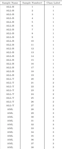
setting page along with other default settings. All parameter settings can be revised to reflect interests of the user. If true class labels are available for a benchmark data set and one is interested in evaluating the performance of various clustering algorithms, this information can be provided as input in the form of a tab-delimited, text file containing the column (or row) number of the sample and its class label. Class labels should be specified in ordered, numeric format such as 1,2,3 etc. Table 6 illustrates this file format using the leukemia data

set in §6.1.1 as an example. In this table, the first column represents the three subgroups

-ALL-B, ALL-T and AML; the second column specifies sample number and the third column

specifies class labels for the sub-groups (see §6.1.1 for more details). Details of input data

5.2 NMF simulation

The NMF runs are managed as a series of executions of computing units where each

com-puting unit is a matrix factorization process, i.e. from W/H initialization to factorizing V

into the finalW/H based on some criterion. The computing unit is distinct for differentk, or

same k but different W/H initialization. In desktop mode, all computing units are executed

sequentially if only one core is used, or these computing units are distributed and executed in parallel using multiple cores; however in HPC mode, these computing units are

automat-ically distributed and executed in parallel. In the model selection phase, each k is assigned

a job unit to compute the evaluation metrics. These job units are also run in parallel in the HPC mode.

5.3 Initial Scaling and Normalization

In order to speed up convergence, an initial scaling and normalization option is available

for the input W and H matrices. This procedure is aimed at bringing each element of the

initial product matrix W H closer to the corresponding element of the input matrix V and

is implemented in the following steps.

• For each (i, j)th element of V and W H, compute the scale as sW =

1

np

∑ i,j

{Vij/(W H)ij}

wherenp is the number of elements in V orW H.

• Multiply (scale) each element of the matrixW bysW.

• After scaling, the magnitude of elements inW H and V should be similar.

Normalization of the H matrix is intended to maintain the scale of each element of H

across iterations for a given run and across multiple runs of the NMF algorithm. This results

in comparableH matrices and facilitates proper computation of connectivity and consensus

matrices. Normalization is applied to each row ofHfollowed by each column ofW as follows.

• For theath row of H, the scale is computed as sHa =

∑ jHaj.

• Update each element in theath _{row ofH as H}new

a,j =

Hold

a,j

sHa

.

• Update each element in theath _{column ofW as W}new

i,a =Wi,aold·sHa.

There is also an option available to idealize the input matrix by adding a small positive constant to the zero entries in order to provide numerical stability to the algorithm. Initial

scaling, idealization and normalization of W andH are available as separate options. There

5.4 Result retrieval and visualization

NMF based on multiple runs creates several output files in the directory in which the input

data resides and from which hpcNMF is invoked. A summary of results based on the

pre-specifiedN runs are presented in a log file while a summary of results obtained for individual

runs is captured in a separate file. Examples of the former are Tables 2, 3 and 4 shown in the

Examples section. The factored W and H matrices across N runs are captured in separate

files for each rankkwithin a specified range (and for eachαin Renyi divergence). In addition,

the re-ordered consensus matrix from N runs, the final cluster assignments and ordering of

samples are all captured in separate files for eachk andα. All output files are created in (or

can be opened in) tab-delimited, text format. Result retrieval for all three versions is done in this format.

In the currently available web-interface, all intermediate files can be viewed through the web browser. Since the entire process could take anywhere from a few minutes to a few hours to complete, depending on the size of the job, the web server is designed to ask for the user’s email in order for results to be delivered as a web-link. Through this link, users can view

a summary of results, view or download W/H output files, and also view and evaluate the

performance of the factorization through heat maps.

5.5 Performance

We tested hpcNMF on the Linux cluster, Windows desktop as well as on Mac OS X based

on real-life data sets from various applications. A variety of scenarios were considered

de-pendent on the size of the input data matrixV, the range of rankk of the factorization, the

algorithm employed and choices of the parameterαin Renyi divergence; and single-threaded,

multi-threaded and MPI implementations were tested. The results showed thathpcNMF can

reproduce the simulations performed by Matlab and R with a considerable increase in

com-putational speed for all implementations. Table 1 summarizes the performance of hpcNMF

on a HPC cluster consisting of a total of 70 nodes where each node contains anywhere from 2 to 16 Intel Xeon cores (processors) with RAM varying from 1Gb to 92Gb depending on the queue. In this cluster, MPI jobs can recruit cores from more than one node while non-MPI

jobs can use only the cores of the node they are running on. In this table, p and n denote

the number of rows and columns, respectively, of the input data matrix V and data set size

is determined by the product np. The number of individual jobs for a particular data set

(corresponding to each row in Table 1) is based on the number of ranksk in its chosen range

(and the number of values of the parameter α in Renyi divergence). Computational speed

was quantified using three objective measures, namely, the mean number of updates, wall clock time and CPU time required to complete the factorizations. Model selection using con-sensus clustering and a quantitative evaluation of factorizations for a particular algorithm

algorithm. Each run is allowed a maximum of 2000 iterations for convergence and 50−200 runs were typically used in the computations for the examples presented. A run that fails to

converge within this pre-specified limit stops after 2000 iterations and the resulting W and

H matrices are utilized in further quantitative evaluation of clustering.

The mean number of updates per run and wall clock time are objective measures of com-putational speed. The former will affect comcom-putational time depending on the size of the data set while the latter gives a more realistic assessment of computational time required

for a particular job depending on several factors such as data set size, rank k of the

factor-ization, number of runs N and number of choices of α in Renyi divergence. This is due to

parallel implementation of the outlined algorithms on HPC clusters. Wall clock time is also dependent on the number of cores (processors) chosen or available for a particular job on the cluster. CPU time may be affected by the number of available nodes and the demands on the HPC cluster. Hence wall clock time provides a measure of the expected duration for a particular job subject to constraints on the cluster and job size, and be regarded as a more objective measure of speed that is independent of cluster occupancy. The parallel imple-mentation allows us to pre-specify all the aforementioned parameters prior to initiation of a sequence of jobs pertaining to a given data set. Wall clock and CPU times include time spent in parallel processing across multiple cores in one or more nodes for the multi-threaded and MPI versions. As evidenced by the results displayed in Table 1, a significant improvement in computational time was observed overall due to the parallel implementation. The parallel implementation described in this work should be readily accessible to researchers due to the increased utilization of HPC clusters as part of computational infrastructure (Devarajan et al., 2015).

It is important to note that a truly single-threaded implementation would use only one core for all jobs pertaining to a data set. This is typically how Matlab and R implementations work in the absence of multi-core processors. Each job pertaining to a data set is actually a computation unit in a multi-threaded implementation. One approach to leveraging the availability of multiple cores in a HPC cluster and optimizing the computations is to manage the jobs related to a particular data set using a job scheduler and a web-interface as the front end. The goal is to to minimize time spent in the queue and to appropriately allocate the required cores for a particular data set in a reasonable time frame. Once the input data is uploaded and the parameters are set using the web interface, the interface would decompose (parallelize) the input data and launch the appropriate number of jobs. In this setting, the number of nodes used depends on the size of the input files. It also depends on the queue and may not be reproducible for the same job. However, the number of cores used would be reproducible regardless of the execution queue. Even though each data set can consist of several jobs, each job uses one core and it can be run on any node in the chosen queue. Under ideal conditions, the processing times would be very similar between this web-interface version and the multi-threaded or MPI version, with the latter providing control over the choice of the number of cores/nodes. The web-interface could serve as the default, thus providing a balance between a truly single-threaded and a multi-threaded or

For the NMF algorithm based on Renyi divergence, single threaded hpcNMF runs 2-3 times

faster than R and MATLAB implementations when α is not equal to 1 or close to zero. We

observed that hpcNMF required approximately the same computational time for different

values of α whereas R and MATLAB implementations were very sensitive to the selection

of α in terms of computation cost. The threaded job is more efficient, as a single job it has

less overhead, and so gives better throughput, but it does not save on CPU time. Jobs with multiple threads use more CPU time with even less cumulative wall time.

6 Examples

We provide several examples illustrating the breadth and depth of applicability ofhpcNMFto

real-life biological and text-mining data sets. The examples are primarily used to demonstrate

the performance ofhpcNMFas the number of rowsp, columnsn, rank factorizationk, choice

of α and type of algorithm are varied, and include the analysis of benchmark data sets in

gene expression and text mining as well as an application in statistical signal processing. Results are displayed in Table 1-5 under a variety of scenarios.

6.1 Gene Expression

6.1.1 Leukemia data

The ALL-AML leukemia data presented in Golub et al. (1999) has become a benchmark data set for illustration of methods for gene expression data. This data set contains gene expres-sion measurements from 38 patient tissue samples on 5000 genes obtained using Affymetrix microarrays. Of these 38 samples, 27 and 11 samples are of ALL and AML type, respec-tively. The 27 ALL samples are further divided into 19 T-type and 8 B-type, thereby rep-resenting a hierarchical structure. Brunet et al. (2004) used the Poisson model-based NMF

algorithm (KL divergence, i.e., α = 1 in eqn. (2.4)) together with consensus clustering to

analyze this data set, and further showed that this algorithm outperformed the Gaussian

model-based algorithm. It is well known that factorizations of ranks k = 2,3 delineates

the samples into ALL-T, ALL-B and AML sub-types. The Poisson model-based NMF

al-gorithm using generalized Renyi divergence (that includes KL divergence when α = 1)

was applied to this data and evaluated for 11 different choices of α in the range (0,10]

for factorizations of ranks k = 2,3,4,5. There is some evidence in the literature

suggest-ing that data obtained from ssuggest-ingle-channel microarray platforms such as Affymetrix ex-hibit a heavy right-tailed distribution such as a gamma (Devarajan et al., 2005, 2006, 2008; see also http://discover.nci.nih.gov/microarrayAnalysis/Microarray.Home.jsp). Therefore we also applied a gamma model-based NMF algorithm to this data.

algorithms and choices of the parameters k and α specified above. It also includes an as-sessment of the computational performance for the Gaussian and gamma model-based NMF

algorithms outlined in this paper. Table 2 lists the various metrics computed by hpcNMF

to evaluate the homogeneity of clustering and quality of reconstruction for these parameter

choices based on the Poisson model. For a rank k = 2 factorization, α = 0.5 is the best

performing model with a misclassification rate of 2.63% (ν = 6.38%); and for a rank k = 3

factorization, α = 0.25 is the best performing model with a misclassification rate of 2.63%

(ν = 6.62%). This is corroborated by the highest estimated values of ARI and NMI among

choices of α for k = 2,3. This result compares with a misclassification rate of 5.26% based

on the standard Poisson algorithm using KL divergence (α = 1) for k = 2,3 (ν = 11.95%

and 12.02%, respectively). The homogeneity of clustering for these four cases is illustrated

by heat maps of the respective re-ordered consensus matrices in Figures 1-4. If the true class

labels were not known, ρ, κ and the Spearman version of ρ, ˜ρ, would provide a means for

assessing the homogeneity of clustering and aid in selecting an appropriate model. As seen from Table 2, there are several competing models the most homogeneous of which are either

based on a rankk = 2 or k = 3 factorization.

For a given rank k, the mean number of updates is seen to increase with α while mean

sparseness of metagenes and metagene expression patterns are observed to slightly decrease

with α. However, for a given α, mean sparseness is observed to increase with rank k. It

is interesting to note that both κ and ˜ρ exhibit a wider and practically more useful range

of (0.54,1) across k than ρ itself ((0.93,1)). For lower ranks (k = 2,3), the convergence

rate of the algorithm is very high with the exception of α = 10 for k = 2 and α = 4,10

for k = 3. The convergence rate is generally seen to be lower with higher ranks and rapidly

declines with increasingα. Metrics such as the mean number of updates, reconstruction error,

convergence rate and ϵ serve as useful diagnostic tools in assessing the overall performance

of the algorithms both in terms of speed and accuracy.

6.1.2 Glioma data

Nutt et al. (2003) described a gene expression data set on gliomas obtained from 50 pa-tient samples using Affymetrix microarrays. The raw data was pre-processed and quantile normalized using the RMA approach (Bolstad et al., 2003). Genes exhibiting a coefficient of variation in excess of 50% across the samples were retained. This resulted in a data set containing expression profiles of 972 genes thereby providing an appropriate size for illus-trating our approach. This set was used to demonstrate the applicability of our methods and to compare the performance of various NMF algorithms. Algorithms based on the Pois-son, gamma and Gaussian models were applied to this data set using factorizations of ranks

k = 2,3, ...,10 in order to identify homogenous sub-groups of genes.

Details of the algorithms employed and their computational times are provided in Table 1 while the results of this analysis are summarized in Table 3. It is evident from Table 3 that,

able to explain the variation in the data better than that based on the Gaussian model. In

terms of mean number of updates, reconstruction error, convergence rate and ϵ, the gamma

model exhibits superior performance relative to other models. The Gaussian model-based algorithm is observed to not converge within the maximum allowable 2000 iterations per run

for all ranks with the exception of k = 2 while the Poisson (KL) model-based algorithm is

observed to generally require a large number of iterations per run to achieve convergence and closer to 2000 iterations per run for higher ranks. On the other hand, the gamma model-based algorithm is seen to converge in significantly fewer iterations across all ranks. It is interesting

to note that the sparseness of the metagene coefficients (W) is similar across different models

for a given rankk factorization. On the other hand, the gamma and Poisson models result in

sparser metagene expression profiles (H) across ranks k with the gamma model producing

the sparsest H particularly with increasing rankk. It is evident from Table 3 that clustering

homogeneity generally declines with increasing k; however, both these models suggest the

presence of six homogeneous clusters of genes, based on ρ and κ, thus requiring further

investigation of the biological relevance of these sub-groups.

6.2 Text Mining

Text mining is concerned with the recognition of patterns or similarities in natural language

text. Consider a corpus of documents that is summarized as a p×n matrix V in which

rows represent terms in the vocabulary, columns correspond to documents in the corpus and the entries denote frequencies of words in each document. In document clustering studies,

the number of terms p is typically in the thousands and the number of documents n is

typically in the hundreds. The objective is to identify subsets of semantic categories and to cluster the documents based on their association with these categories by finding a small

number of metaterms, each defined as a nonnegative linear combination of the p terms.

This is accomplished by decomposing the frequency matrix V into the product of W and H

where each column ofW defines a metaterm and each column ofH represents the metaterm

frequency pattern of the corresponding document. Application of NMF in text mining and document clustering is discussed in Pauca et al. (2004), Shahnaz et al. (2006), Chagoyen et al. (2006) and Devarajan et al. (2015).

6.2.1 Reuters data

The Reuters data is one of the most widely used benchmark data sets in text mining. It contains the frequencies of 1969 distinct terms from 276 different documents, belonging to a total of 20 different categories (Shahnaz et al., 2006; Devarajan et al., 2015). For the

purpose of illustrating the utility of hpcNMF in text mining applications, a subset of this

data consisting of five different categories was used. The subset contains 1163 terms from 82 documents. Data was pre-processed using the methods described in Devarajan et al. (2015). The Poisson model-based NMF algorithm using Renyi divergence (that includes KL

divergence whenα= 1) was applied to this data for various choices of αin the range (0,10] for factorizations of ranks k = 2,3,4,5.

Table 1 lists the computational times for the various algorithms. For the sake of illustration,

detailed results are summarized in Table 4 only for k = 5 since there are five categories of

documents in this subset. The best performing model is achieved for α = 0.5 and results

in the lowest misclassification rate of 20.73% (ν = 31.38%) among all choices of α. This is

also the best performing model in terms of overall cluster consensus κ = 0.84 among all

α. It compares with a misclassification rate of 26.83% (ν = 37.31%) based on the standard

Poisson algorithm using KL divergence (α= 1). Heat maps of the corresponding re-ordered

consensus matrices, shown in Figures 5 and 6, graphically illustrate the homogeneity of clustering for these two cases. Mean sparseness of the metaterms and metaterm frequency

patterns are observed to decrease with increasingα. Again, bothκand ˜ρexhibit a wider and

practically more useful range ((0.32,0.84) and (0.65,0.81), respectively) thanρ((0.95,0.99))

across α. As independent measures of clustering accuracy, both NMI and ARI have

rea-sonably strong correlations with the misclassification rate (−0.78 and −0.69, respectively).

The overall quality of reconstruction measured by mean number of updates, reconstruction

error, convergence rate andϵ all appear to be very good across multiple runs. For a detailed

analysis of the complete Reuters data and various subsets using NMF, the interested reader is referred to Devarajan et al. (2015).

T able 1: P erformance of hp cNMF Dataset p n k Clustering on Mo del Div ergence α Up dates § CPU Time † Clo ck Time ∗ W or H (Sec) (Sec) Leuk emia 5000 38 2-5 H P oisson R eny i 0.1,0.25,0.5, 1387.03 2353.03 232.74 0.75,1,1.5,2,4,10 Leuk emia 5000 38 2-5 H P oisson K L 1.0 1242.4 92.85 13.46 Leuk emia 5000 38 2-5 H Gamma 1 K L -957.7 123.64 18.24 Leuk emia 5000 38 2-5 H Gaussian E D -1999.5 120.28 17.14 Leuk emia 1163 82 2-5 H P oisson R eny i 0.1,0.25,0.5, 97.96 81.13 9.6 0.75,1,1.5,2,4,10 Reuters 1163 82 2-5 H P oisson K L 1.0 71.2 2.43 0.46 Glioma 972 50 2-10 W P oisson K L -1796.13 104.77 13.38 Glioma 972 50 2-10 W Gamma 1 K L -773.02 98.69 15.6 Glioma 972 50 2-10 W Gaussian E D -1961.87 107.17 14.74 EMG 13 11950 2-5 W Gamma 1 K L -749.5 107.17 13.84 EMG 13 11950 2-5 W Gamma K L d -611.1 67.15 10.44 EMG 13 11950 2-5 W Gamma J -899.4 95.41 15.72 EMG 13 11950 2-5 W In v erse Gaussian K L d -1667.5 166.67 28.94 EMG 13 11950 2-5 W Gaussian E D -640.3 35.62 10.2 § Mean n um b er of up dates p er run † Mean CPU time (single core) p er run ∗ Mean w all clo ck time p er run 1 Based on the heuristic algorithm of Cheung & T resc h (2005) and Cic ho cki et al. (2006); all other implemen tations are based on the EM algorithm

T able 2: Leuk emia data -summary of results from rank k = 2 − 5 factorizations using Ren yi div ergence k α ρ κ MC (%) ν ˜ ρ ARI NMI ω C R R E ϵ ψ ( h ) ψ ( w ) Up dates § R 2 2 0.1 1.00 0.99 5.26 0.08 0.97 0.79 0.67 4.3e-5 1 16040700 0.01 0.32 0.64 556.9 0.81 2 0.25 0.99 0.97 5.26 0.07 0.97 0.79 0.67 9.5e-5 1 16165457.5 0.01 0.32 0.64 537.9 0.79 2 0.5 1.00 0.99 2.63 0.06 0.93 0.89 0.83 2.1e-5 1 16290064.5 0.01 0.32 0.64 559 0.78 2 0.75 0.98 0.98 5.26 0.09 0.98 0.79 0.73 5.2e-5 1 16319218 0.01 0.31 0.63 532.4 0.79 2 1 † 1.00 1.00 5.26 0.12 0.98 0.79 0.73 6e-6 1 16272485 0.01 0.31 0.63 532.7 0.82 2 1.5 1.00 1.00 5.26 0.12 1.00 0.79 0.73 0 1 16007066 0.01 0.30 0.63 710.8 0.88 2 2 0.98 0.89 5.26 0.21 0.90 0.79 0.73 32.2e-5 1 15700254 0.01 0.29 0.62 733.4 0.95 2 4 0.96 0.85 5.26 0.25 0.88 0.79 0.73 44.8e-5 0.98 13380638 0.06 0.29 0.62 1202.8 1 2 10 0.93 0.74 10.53 0.34 0.90 0.61 0.49 74.3e-5 0.315 8421125.2 25.72 0.27 0.62 1924.1 1 3 0.1 1.00 0.99 2.63 0.08 0.73 0.91 0.91 2.2e-5 0.995 13900000.5 0.01 0.43 0.66 873 0.83 3 0.25 1.00 1.00 2.63 0.07 0.79 0.91 0.91 1e-5 1 13940044.5 0.01 0.43 0.66 856.2 0.82 3 0.5 1.00 0.98 2.63 0.08 0.73 0.91 0.91 5.1e-5 0.995 13946100.5 0.01 0.43 0.65 875.3 0.82 3 0.75 1.00 0.99 5.26 0.12 0.71 0.83 0.82 2.9e-5 1 13898748 0.01 0.43 0.65 904.7 0.82 3 1 † 1.00 0.99 5.26 0.12 0.69 0.83 0.82 3.1e-5 1 13806611 0.01 0.43 0.65 946.4 0.84 3 1.5 1.00 0.99 7.89 0.18 0.69 0.75 0.76 3.0e-5 0.99 13490603 0.02 0.42 0.64 1085 0.9 3 2 1.00 1.00 7.89 0.19 0.75 0.75 0.76 4e-6 0.945 13038359 0.57 0.42 0.64 1302.5 0.96 3 4 0.98 0.84 10.53 0.30 0.81 0.68 0.68 33.7e-5 0.305 10967223 10.58 0.41 0.63 1919.5 1 3 10 0.96 0.66 7.89 0.39 0.86 0.75 0.76 71.5e-5 0 6828610.65 37.75 0.38 0.64 2000 1

T able 2 (con tin ued): Leuk emia data -summary of results from rank k = 2 − 5 factorizations using Ren yi div ergence k α ρ κ MC Rate ν ˜ ρ ARI NMI ω C R R E ϵ ψ ( h ) ψ ( w ) Up dates § R 2 4 0.1 0.98 0.92 42.11 -0.67 0.33 0.58 14.9e-5 0.88 12579917 0.06 0.46 0.68 1384.8 0.85 4 0.25 0.99 0.95 42.11 -0.58 0.33 0.58 9.7e-5 0.86 12614524 0.04 0.46 0.68 1476.2 0.84 4 0.5 0.99 0.95 42.11 -0.67 0.33 0.58 9.9e-5 0.8 12617286 0.04 0.45 0.67 1556.7 0.83 4 0.75 1.00 0.98 44.74 -0.54 0.33 0.57 3.6e-5 0.8 12562473 0.29 0.45 0.67 1574.4 0.84 4 1 † 0.99 0.96 44.74 -0.56 0.33 0.57 8.2e-5 0.725 12454671 0.39 0.44 0.67 1620.7 0.86 4 1.5 0.99 0.93 47.37 -0.70 0.27 0.48 12.3e-5 0.535 12090130 0.83 0.45 0.66 1824.7 0.91 4 2 0.98 0.89 50.00 -0.68 0.21 0.38 20.8e-5 0.29 11596174 2.87 0.45 0.65 1926.9 0.96 4 4 0.97 0.81 47.37 -0.78 0.24 0.42 35.4e-5 0.005 9509622.2 14.95 0.46 0.65 1999.7 1 4 10 0.96 0.62 42.11 -0.78 0.26 0.43 70.2e-5 0 5850838.25 26.75 0.44 0.65 2000 1 5 0.1 0.97 0.81 57.89 -0.61 0.17 0.36 33.5e-5 0.735 11570450.5 0.27 0.50 0.69 1635.6 0.86 5 0.25 0.98 0.90 55.26 -0.66 0.21 0.39 18.5e-5 0.75 11600127 0.10 0.50 0.69 1617.4 0.85 5 0.5 0.98 0.90 52.63 -0.60 0.25 0.48 17.5e-5 0.65 11600058.5 0.19 0.49 0.68 1723.6 0.85 5 0.75 0.97 0.90 60.53 -0.56 0.23 0.46 16.8e-5 0.465 11533286 0.71 0.48 0.68 1822.5 0.85 5 1 † 0.96 0.85 60.53 -0.55 0.23 0.46 26.9e-5 0.39 11418070.5 0.82 0.48 0.68 1869.8 0.87 5 1.5 0.97 0.82 60.53 -0.69 0.21 0.43 31.7e-5 0.345 11031964 1.29 0.48 0.67 1886.2 0.92 5 2 0.98 0.81 63.16 -0.70 0.20 0.42 33.9e-5 0.17 10560495.5 2.86 0.48 0.67 1961.1 0.96 5 4 0.97 0.66 47.37 -0.79 0.22 0.41 58.9e-5 0 8557281.85 8.64 0.49 0.66 2000 1 5 10 0.95 0.54 44.74 -0.73 0.23 0.42 8.1e-4 0 5160238.65 33.60 0.48 0.66 2000 1 C R Con v ergence rate R E Reconstruction error † corresp onds to K L div ergence for the P oisson mo del

T able 3: Glioma data -summary of results from rank k = 2 − 10 factorizations Mo del Div ergence k ρ κ ˜ ρ ω C R R E ϵ ψ ( h ) ψ ( w ) Up dates § R 2 Gaussian E D 2 0.98 0.94 0.92 0 1 2052620000 0.01 0.18 0.57 1656.8 0.75 Gaussian E D 3 0.98 0.92 0.91 0 0 1704206800 1701.53 0.24 0.61 2000 0.79 Gaussian E D 4 0.98 0.88 0.86 0 0 1441675800 72.76 0.27 0.65 2000 0.82 Gaussian E D 5 0.99 0.94 0.77 0 0 1208748400 160.10 0.30 0.66 2000 0.85 Gaussian E D 6 0.98 0.91 0.64 0 0 1055399200 867.88 0.32 0.67 2000 0.87 Gaussian E D 7 0.96 0.85 0.70 0 0 943793560 601.98 0.35 0.68 2000 0.88 Gaussian E D 8 0.95 0.80 0.60 1e-6 0 850208460 1274.62 0.37 0.68 2000 0.90 Gaussian E D 9 0.94 0.78 0.57 1e-6 0 768908740 1290.52 0.40 0.69 2000 0.91 Gaussian E D 10 0.94 0.70 0.61 1e-6 0 694673720 1321.73 0.42 0.69 2000 0.91 Gamma K L 2 0.99 0.97 0.92 0 1 5981.43 0.01 0.19 0.56 200.4 0.87 Gamma K L 3 0.98 0.93 0.81 0 1 4999.08 0.01 0.26 0.60 455.2 0.89 Gamma K L 4 0.95 0.82 0.70 1e-6 1 4358.58 0.01 0.34 0.61 569.6 0.90 Gamma K L 5 0.93 0.75 0.70 1e-6 1 3901.51 0.01 0.38 0.62 698.4 0.91 Gamma K L 6 0.96 0.80 0.65 1e-6 0.98 3509.13 0.01 0.41 0.62 816.4 0.92 Gamma K L 7 0.94 0.76 0.59 1e-6 0.98 3194.47 0.01 0.45 0.63 966.4 0.93 Gamma K L 8 0.93 0.67 0.57 1e-6 0.96 2954.49 0.01 0.48 0.64 1054 0.93 Gamma K L 9 0.93 0.68 0.54 1e-6 0.96 2744.43 0.01 0.51 0.64 1076.8 0.94 Gamma K L 10 0.94 0.70 0.51 1e-6 1 2549.56 0.01 0.53 0.65 1120 0.94

T able 3 (con tin ued): Glioma data -summary of results from rank k = 2 − 10 factorizations Mo del Div ergence k ρ κ ˜ ρ ω C R R E ϵ ψ ( h ) ψ ( w ) Up dates § R 2 P oisson K L † 2 0.99 0.96 0.93 0 1 1287643.8 0.01 0.19 0.55 1188.4 0.86 P oisson K L 3 0.98 0.95 0.76 0 0.82 1096008.8 0.02 0.25 0.59 1500.4 0.88 P oisson K L 4 0.94 0.80 0.69 1e-6 0.74 958925.9 0.04 0.30 0.60 1566 0.89 P oisson K L 5 0.98 0.86 0.68 0 0.24 861127.42 0.26 0.35 0.61 1950.8 0.90 P oisson K L 6 0.99 0.94 0.59 0 0.08 770833.18 0.50 0.38 0.63 1964.8 0.91 P oisson K L 7 0.97 0.85 0.53 0 0.02 705069.52 0.41 0.40 0.65 1995.2 0.92 P oisson K L 8 0.98 0.91 0.53 0 0.04 643798.96 0.88 0.42 0.66 1999.6 0.93 P oisson K L 9 0.95 0.76 0.51 1e-6 0 595497.56 0.86 0.44 0.66 2000 0.93 P oisson K L 10 0.95 0.69 0.48 1e-6 0 550793.06 0.71 0.46 0.67 2000 0.94 † corresp onds to α = 1 in Ren yi div ergence for the P oisson mo del, k = 2 − 10