Capacity Planning
Sales and Operations Planning •Forecasting
•Capacity planning •Inventory optimization
•How much capacity assigned to each production unit? •Realistic capacity estimates
•Strategic level
•Moderately long time horizon •Larger time buckets
•Data not known exactly
1
Operations Planning
•Pochet-Wolsey’s model is too large, NP-hard •Decomposition→inaccurate model
•Medium-term planning horizon, strategic level •Larger time buckets
2
Some definitions
•Work in Process inventory between the start and end
points of a product routing is called work in process (WIP)
•WIP inventory work in process inventory
•FGI inventory final goods inventory
•Lead time of a given routing or line is the time allotted
for production of a part on that routing or line.
•Littles Law
WIP=Throughput×cycle time
Master Production Scheduling Model (Pochet-Wolsey)
•time horizon t=1, . . . ,n
•φi
tunit production cost •qtifixed production cost •πi
tinventory cost •Di
tdemand Decision variables
•xtiproduction lot size in period t
•ytibinary variable indicating production period t •Ii
t inventory at end of period t Moreover
•Ck
t available capacity, resource k time t •ξikper unit resource consumption •βikfixed resource consumption
Material Requirement Planning Model (Pochet-Wolsey)
Multi-item multi-level capacitated lot-sizing model •Optimize simultaneously production and purchase of
all items
•from raw materials to finished products •satisfy external demands
•satisfy internal demands •short-term horizon Bill of materials (BOM)
5
Material Requirement Planning Model (Pochet-Wolsey)
•S(i)set of direct successors of i (items consuming i) •ri jamount of item i required to make one item j •γilead-time to produce or deliver a lot of i
i.e. xitcan be delivered at time t+γi
Model min m
∑
i=1 n∑
t=1 φi txti+qityit+πitIti Subject to: Iti−1+x i t−γi= D i t+∑
j∈S(i) ri jxtj ! +Iti ∀i,t xit≤Mtiyit ∀i,t m∑
i=1 ξikxi t+ m∑
i=1 βikyi t≤Ctk ∀t xit∈R+,Iti∈R+,yti∈ {0,1}Large, NP-hard model, difficult to solve
6
Capacity of Resources
•Gross capacity •Usable capacity •Productivity factor
Resource Gross Productivity Usable Description Capacity Factor Capacity
(hours/day) (hours/day)
Machine S100 8 0.95 7.6
Forklift 8 0.85 6.8
Machine ASS 16 0.85 13.6
Machine PPP 8 0.95 7.6
Capacity limit is soft (queuing theory) Capacity depends on - variation in arriving jobs - variation in lead times Lead time depends on load
Asmundsson, Single-stage multi-product planning
Simplified model min
∑
i∑
t φitXit+πitIit Subject to: Iit=Ii,t−1+Xi,t−L−Dit ∀i,t∑
i ξitXit≤Ct ∀t Xit,Iit∈R+ ∀i,t•LP-model (easy to solve)
•Setup times are neglected (future work) •Constant lead time (production time) L
Introduction
Accurate measurements of manufacturing capacity is hard to obtain (Elmaghraby 1991)
•Stochastic performance analysis models
Queuing models capture important aspects (Hopp, Spear-man 2000)
Stochastic model of whole production unrealistic •Deterministic techniques
Divide planning horizon in discrete buckets Assign capacity in each bucket
Solution satisfying aggregated constraint not feasible in practice
•Integrating approaches (Hung, Leachmand 1996) Solve LP model for production planning
Feed into simulator to estimate lead times Add cut if not feasible
nonlinear clearing function.
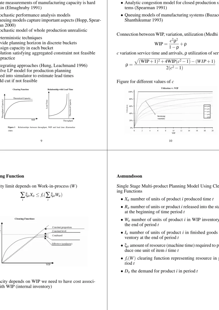
Figure 1 Relationships between throughput, WIP and lead time (Karmarkar 1989) Clearing Function WIP T h ro u g h p u t (C ap ac it y ) L ea d T im e Throughput Relationship with Lead Time
Theoretical Capacity T h eo re ti ca l C ap ac it y 9
Relation between WIP and system throughput
•Analytic congestion model for closed production sys-tems (Spearman 1991)
•Queuing models of manufacturing systems (Buzacott, Shanthikumar 1993)
Connection between WIP, variation, utilization (Medhi 1991) WIP= c
2ρ2
1−ρ+ρ
c variation service time and arrivals,ρutilization of server
ρ=
p
(WIP+1)2+4WIP(c2−1)−(W IP+1)
2(c2−1)
Figure for different values of c
10
Clearing Function
Capacity limit depends on Work-in-process (W )
∑
i
ξitXit≤ ft(
∑
i
ξitWit)
If capacity depends on WIP we need to have cost associ-ated with WIP (internal inventory)
Asmundsson
Single Stage Multi-product Planning Model Using Clear-ing Functions
•Xitnumber of units of product i produced time t •Ritnumber of units or product i released into the stage
at the beginning of time period t
•Wit number of units of product i in WIP inventory at the end of period t
•Iit number of units of product i in finished goods in-ventory at the end of period t
•ξitamount of resource (machine time) required to pro-duce one unit of item i time t
• ft(W)clearing function representing resource in pe-riod t
CF model (Clearing Function) min
∑
t∑
i φitXit+ωitWit+πitIit+ρitRit Subject to: Wit=Wi,t−1−Xit+Rit ∀i,t Iit=Ii,t−1+Xit−Dit ∀i,t∑
i ξitXit≤ ft(∑
i ξitWit) ∀t Xit,Wit,Iit,Rit∈R+ ∀i,t where•φitcost of producing unit i time t •ωitcost of WIP of unit i time t •πitcost of inventory unit i time t •ρitcost of releasing unit i time t
13
Problem with capacity constraint
XA+XB≤f(WA+WB)
for two products A,B
•Solution exists XA>0, XB=0, WA=0, WB>0 •Maintain high WBif cheap
•Create capacity for XA
No link between WIP available and production
14
Solution
Zit≥0 represent an allocation of expected throughput among different products Xit≤Zitft(
∑
i ξitWit) ∀i,t∑
i Zit=1 ∀tDepends on total WIP.
Prefer WIP of specific product i.
AssumingξitWit=Zit∑iξitWitwe get (?) Xit≤Zitft( ?
∑
i ξitWit Zit ) ∀i,t∑
i Zit=1 ∀t WIP T h ro u g h p u t (C ap ac it y ) Theoretical CapacityACF model (Allocated Clearing Function)
min
∑
t∑
i φitXit+ωitWit+πitIit+ρitRit Subject to: Wit=Wi,t−1−Xit+Rit ∀i,t Iit=Ii,t−1+Xit−Dit ∀i,t Xit≤Zitft( ?∑
i ξitWit Zit ) ∀t∑
i Zit=1 ∀t Xit,Wit,Iit,Rit∈R+ ∀i,tOuter approximation of clearing function
Outer linear functionsαcWt+βcfor c=1, . . . ,C
∑
i ξitWit≤αcWt+βc ∀c,t then f(W) = min c=1,...,C{α c Wt+βc} Assume that α1 >α2>α3> . . . >αc=0 Linear model min∑
t∑
i φitXit+ωitWit+πitIit+ρitRit Subject to: Wit=Wi,t−1−Xit+Rit ∀i,t Iit=Ii,t−1+Xit−Dit ∀i,t∑
i ξitXit≤αcξitWit+Zitβc ∀i,t,c∑
i Zit=1 ∀t Zit,Xit,Wit,Iit,Rit∈R+ ∀i,tWhich is correct since
Zitf ξ itWit Zit = Zitmin c αcξitWit Zit +βc = min c {α cξ itWit+βcZit} 17
Asmundsson, experimental results
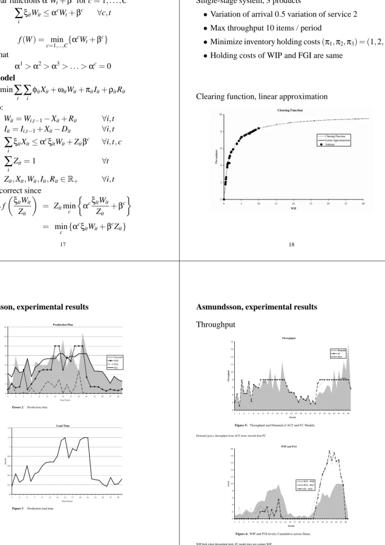
Single-stage system, 3 products
•Variation of arrival 0.5 variation of service 2 •Max throughput 10 items / period
•Minimize inventory holding costs(π1,π2,π3) = (1,2,3)
•Holding costs of WIP and FGI are same
Clearing function, linear approximation
18
Asmundsson, experimental results Production Plan 0 2 4 6 8 10 12 14 1 3 5 7 9 11 13 15 17 19 21 23 25 27 29 Time Period Demand WIP FGI TH
Figure 2 Production plan
Lead Time 0 0.2 0.4 0.6 0.8 1 1.2 1.4 1 3 5 7 9 11 13 15 17 19 21 23 25 27 29 Time Period P er io d s
Figure 3 Production lead time
5 Conclusions
Asmundsson, experimental results
Throughput Throughput 0 2 4 6 8 10 12 14 16 18 1 3 5 7 9 1113 151719212325 2729 3133353739 41434547 49 Period Throughput Demand FC PCF
Figure 5: Throughput and Demand of ACF and FC Models.
Demand (gray), throughput from ACF more smooth than FC
WIP and FGI
0 2 4 6 8 10 12 14 16 18 20 1 3 5 7 9 1113151719212325272931333537394143454749 Period Level PCF - WIP PCF - FGI FC - FGI
Figure 6:WIP and FGI levels, Cumulative across Items.
WIP high when throughput high, FC model does not capture WIP
Asmundsson, experimental results Lead-Time 0.00 1.00 2.00 3.00 4.00 5.00 6.00 7.00 8.00 0 5 10 15 20 25 30 35 40 45 Period Lead-Time Item 1 Item 2 Item 3 Average Raw Processing
Figure 7:Production Lead-Time across all Items.
lead time greater than 0.1 (raw processing time), varies significantly
Marginal Cost of Capacity
0 5 10 15 20 25 1 3 5 7 9 1113151719212325 272931333537394143454749 Period MMC PCF FC
Figure 8:Marginal Cost of Capacity (MCC).
capacity constraint active in ACF, marginal cost positive
marginal cost is zero in FC for all periods where FGI is zero
21
Asmundsson, experimental results
Lead-Time vs. Throughput 0.00 0.20 0.40 0.60 0.80 1.00 1.20 0 1 2 3 4 5 6 7 8 9 10 Throughput Lead-Time
Figure 9:Nonlinear Relationship between throughput and lead time