An Ensemble Data Mining and FLANN
Combining Short-term Load Forecasting System
for Abnormal Days
Ming Li
College of Automation, Guangdong University of Technology, Guangzhou, P.R.China Email: [email protected]
Junli Gao
College of Automation, Guangdong University of Technology, Guangzhou, P.R.China Email: [email protected]
Abstract—The modeling of the relationships between the power loads and the variables that influence the power loads especially in the abnormal days is the key point to improve the performance of short-term load forecasting systems. To integrate the advantages of several forecasting models for improving the forecasting accuracy, based on data mining and artificial neural network techniques, an ensemble decision tree and FLANN combining short-term load forecasting system is proposed to mainly settle the weather-sensitive factors’ influence on the power load. In the proposed strategy, an ensemble decision tree with abnormal pattern modification algorithm and a FLANN algorithm are used respectively to obtain the initial predicting results of the power loads first, a BP-based combination of the above two results are used to get a better prediction afterwards. Corresponding forecasting system is developed for practical use. The statistical analysis showed that the accuracy of the proposed short time load forecasting of abnormal days has increased greatly. Meanwhile, the actual forecast results of Anhui Province’s electric power load have validated the effectiveness and the superiority of the system.
Index Terms—short-term load forecasting, combining forecasting, abnormal days, ensemble data mining, FLANN
I. INTRODUCTION
Power load forecasting is of great importance in power system design in the sense that the prediction accuracy will directly affect the operation and planning of the whole power load system. In the past few decades, a variety of power load forecasting algorithms have been proposed and revised, such as neural networks[1], expert systems[2], fuzzy systems approach[3], SVM[4], data mining[5], etc. However, these methods did not consider the accumulation effect of meteorological character especially with the unusual weather conditions and varied
holiday activities; here we call “Abnormal Days”. So, due to the complexity and uncertainty, it is hard to model the relationships between the loads and related variables. The difficulties may exit in the following aspects: first of all, the modeling and the parameters’ choosing are troublesome for the lack of adequate cognition of the influencing mechanism of the load; second, The load at a given day is dependent on too much factors, e.g. it may be influenced by the load at the previous day or the same day in the previous week[6]; furthermore, the unexpected events will cause fluctuations in the power load, etc.
Toward the major factors which make the modeling process complicated, a combining forecasting strategy based on similarity is proposed in this paper to solve the problem. First, an ensemble data mining with abnormal pattern modification algorithm and a FLANN technique are used respectively to obtain the initial results. Then, a BP-based combination of the above two results are used to get a better prediction. The method has an advantage of dealing not only with the nonlinear part of load, but also with the abnormal days with rapid climate change.
The paper is organized as follows: Part II introduces the system design, including the architecture and the two main modules; the core algorithms of the ensemble data mining, the FLANN and the final combining are focused on in Part III, detailed implementation is discussed to clarify the key points; application and results are illustrated to validate the proposed system in Part IV, then a conclusion is drawn in Part V with some suggestions of the future research..
II. SYSTEM DESIGN
A. Overall Architecture
The overall architecture of the combining short-term load forecasting for Anhui province is shown in Fig. 1. The system uses the Server-Client architecture and MS SQL database. It consists of two modules: The Data Processing Module and the Load Forecasting Module. Data Processing Module is to convert the load data and Manuscript received Oct. 1st, 2010; revised Oct. 20th, 2010;
accepted Nov. 5th, 2010.
This work is supported by the 211 Funding in Guangdong Province, Guangdong Development and Reform [431] and the Dr. Start Fund in Guangdong University of Technology
meteorological data into the specific form of training data required by the data mining algorithms; the Load Forecasting Module’s task is to call the data mining the FLANN and the combining algorithms for the loads prediction, which can be easily browsed by the client.
The system will first load the power load data and the data of all the relevant factors which will influence the power load. After the preprocessing, cleaning, and analyzing of the loaded data, selected algorithm will be running to obtain the model of relevant factors’ quantified impact on the load, especially the hidden patterns which will be revealed and modeled in part III. Then using the historical load curve data, meteorological data and tomorrow's weather forecast data as the model input, the tomorrow's load curve can be predicted.
Figure 1. System Architecture
B. Data Processing Module
The data we used includes the power load and the meteorological data. These two data are in two forms: the historical data and real-time data. For the power load data, the historical data and the real-time data are in the same format, collecting one record per 15 minutes. As for the meteorological data, the historical data is the validated data with high accuracy and good integrity which have been checked by the Meteorological Department, but the data density is low (6 hours a meteorological record) and the real-time data is collected according to the real-time measurement. Opposite to the historical data, it always has more error data and missing data, but the data density is high, collecting one record per 1 hour.
Data Pretreatment
In order to process these data into the form we desired the necessary pretreatment of the data includes[7]:
(a) Error data. Remove error data deviating from the valid range, e.g. we treated the power load p>0 and the valid temperature value is T∈[-20°C 40°C]
(b) Missing data. There are missing data in database and the removed error data will also cause new missing dada. Thus a linear interpolation method is used to fill the missing position when the interval is relative short, e.g. when the data on time n and n+i are known, then the data on n+j is as follows: Tn+j=Tn+(Tn+j-Tn)·j/i. Meanwhile,
when the interval is relative long, the missing data can be replaced by the data of recent days or similar days.
(c) Data density conversion. This rule is mainly for the meteorological data. As stated above, the power load data
is one record per 15 minutes while weather data is one record per six hours. The results of conversion are both one record per fifteen minutes.
Attributes Selection
Regardless of the learning mechanism, the condition attributes and the target attributes should be determined first. The gray relevant analysis results have shown that the meteorological factor is the most important one in the factors influencing the load. From the province’s 3 years’ large regional meteorological load database, according to the suggestions of the power experts and the meteorologists, the temperature, relative humidity, total cloud cover, rainfall, vapor pressure and maximum gust speed are adopted as the condition attributes, which are basically covers the main meteorological factors that affect the load.
In order to reflect the attributes’ change’s impact on the power load, the value of meteorological changes is used here. And, the changes do not mean the difference between adjacent two days, but the difference compared to the day before yesterday. Meanwhile, considering that the load is not only depend on the meteorological changes, but also their baseline value, e.g. if increasing 3℃, its impact on the load is significantly different in the summer from the winter, so the meteorological baseline value are also used here. In summary, a total of 12 meteorological attributes is set to be the input properties.
Although the original meteorological data of 16 cities in the province can be more fully reflect the province's meteorological conditions, but if so, the resulted attributes are too much (16·12=192), which will make the prediction complicated. So according to the geographical distribution of Anhui Province, the 16 cities have been divided into three regions: Huaibei, Jiangnan and Jianghuai. Thus, a total of 36 meteorological properties are treated in this way.
The nest step is to determine the target attribute. As the power load changes shows a regular trend, we define a load changing rate as the target attribute to reflect this change: 2 100% n n n n p p p p + − Δ = ⋅ (1)
where Pn+2, Pn are the power load of the (n+2)th day and
the nth day respectively.
C. Power Load Forecasting Module
A combining forecasting with adaptive coefficients is used to produce more accurate load prediction by sharing the strength of different predictions. The challenges exist in two aspects: the first is how to reflect the influence factors’ impact on the power load, especially the unusual change in abnormal days. The second is how to find the best nonlinear combination of the two methods so as to outperform the individual forecast.
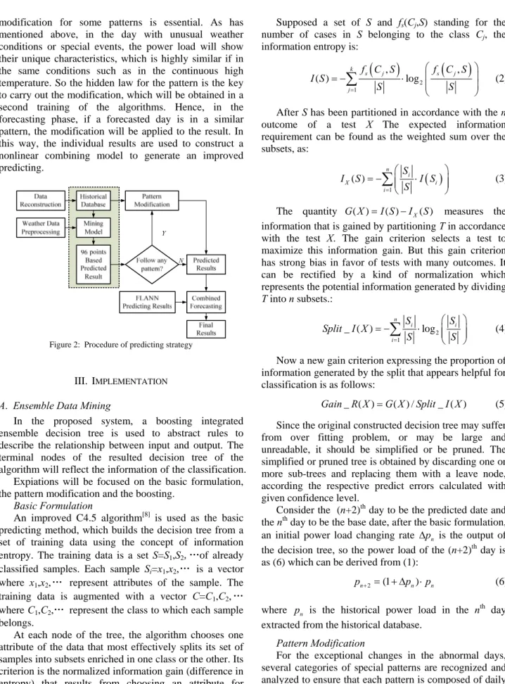
By comparing the various predicting algorithms, taking the actual situation in power load forecasting into account, an ensemble decision tree and FLANN combining algorithm is proposed as Fig. 2 shows. We can use each algorithm to get two independent predictions. Next,
modification for some patterns is essential. As has mentioned above, in the day with unusual weather conditions or special events, the power load will show their unique characteristics, which is highly similar if in the same conditions such as in the continuous high temperature. So the hidden law for the pattern is the key to carry out the modification, which will be obtained in a second training of the algorithms. Hence, in the forecasting phase, if a forecasted day is in a similar pattern, the modification will be applied to the result. In this way, the individual results are used to construct a nonlinear combining model to generate an improved predicting.
Figure 2: Procedure of predicting strategy
III. IMPLEMENTATION
A. Ensemble Data Mining
In the proposed system, a boosting integrated ensemble decision tree is used to abstract rules to describe the relationship between input and output. The terminal nodes of the resulted decision tree of the algorithm will reflect the information of the classification. Expiations will be focused on the basic formulation, the pattern modification and the boosting.
Basic Formulation
An improved C4.5 algorithm[8] is used as the basic predicting method, which builds the decision tree from a set of training data using the concept of information entropy. The training data is a set S=S1,S2,…of already
classified samples. Each sample Si=x1,x2,… is a vector
where x1,x2,… represent attributes of the sample. The
training data is augmented with a vector C=C1,C2,…
where C1,C2,… represent the class to which each sample
belongs.
At each node of the tree, the algorithm chooses one attribute of the data that most effectively splits its set of samples into subsets enriched in one class or the other. Its criterion is the normalized information gain (difference in entropy) that results from choosing an attribute for splitting the data. The attribute with the highest normalized information gain is chosen to make the decision. The C4.5 algorithm then recurs on the smaller sub lists.
Supposed a set of S and fs(Cj,S) standing for the
number of cases in S belonging to the class Cj, the
information entropy is:
(
)
(
)
2 1 , , ( ) log k s j s j j f C S f C S I S S S = ⎛ ⎞ ⎜ = − ⋅ ⎜ ⎝ ⎠∑
⎟ ⎟ (2) After S has been partitioned in accordance with the n outcome of a test X The expected information requirement can be found as the weighted sum over the subsets, as:( )
1 ( ) n i X i S i I S I S = ⎛ ⎞ = − ⎜⎜ ⋅ ⎝ ⎠∑
S ⎟⎟ (3)The quantity G X( )=I S( )−I SX( ) measures the information that is gained by partitioning T in accordance with the test X. The gain criterion selects a test to maximize this information gain. But this gain criterion has strong bias in favor of tests with many outcomes. It can be rectified by a kind of normalization which represents the potential information generated by dividing T into n subsets.: 2 1 _ ( ) log n i i S S Split I X S S = ⎛ ⎞ = − ⋅ ⎜⎜ ⎝ ⎠
∑
i ⎟⎟ (4) Now a new gain criterion expressing the proportion of information generated by the split that appears helpful for classification is as follows:_ ( ) ( ) / _ ( )
Gain R X =G X Split I X (5)
Since the original constructed decision tree may suffer from over fitting problem, or may be large and unreadable, it should be simplified or be pruned. The simplified or pruned tree is obtained by discarding one or more sub-trees and replacing them with a leave node, according the respective predict errors calculated with given confidence level.
Consider the (n+2)th day to be the predicted date and the nth day to be the base date, after the basic formulation, an initial power load changing rate is the output of the decision tree, so the power load of the (n+2)th day is as (6) which can be derived from (1):
n p Δ 2 (1 ) n n p + = + Δp ⋅pn (6)
where is the historical power load in the nth day extracted from the historical database.
n p
Pattern Modification
For the exceptional changes in the abnormal days, several categories of special patterns are recognized and analyzed to ensure that each pattern is composed of daily load data sequence with highly similar features; then learned modification rules are applied to the data in these patterns, the specific modification is as follows.
Despite the dry bulb temperature and its change are the effective parameters describing the temperature; it can be found that the sensitivity of predictive value varies greatly due to the different times in a day, meanwhile, the temperature parameters’ impact on the load forecasting under different conditions also changes a lot. In view of this situation, the weighted daily maximum temperature is used to reconstruction historical data, which is treated as part of the input to enter the mining model as follows:
Tw(t)=T(t) ×(1-ω)+Tmax×ω (7)
In (7), Tw(t) is the weighted temperature, T(t) is the
dry bulb temperature at time t, Tmax is the highest daily
temperature, ω is the weighting coefficient. The same way is applied to the weather forecasting data processing.
During the system design, only the historical temperature data from June to September is reconstructed using the weighted daily maximum temperature rule, while dry bulb temperature is still used for other times.
It can be seen from (7) that the same form of weighting is implemented regardless of the day and night. Moreover, in the valid context of the weighting coefficients
ω
, night time will be affected more byω
, which is also indicated by the experiment. So if reasonably selected, the weighting coefficients can not only effectively deal with the particularity of the summer temperature, but also weaken the load forecasting’s dependence on accuracy of the weather forecast data, so after this conversion, the impact of people's subjective is considered to improve the system’s performance.It is needed to be mention that, a too small weighting coefficient will not achieve the desired effect and a too big one will weaken the impact of the actual temperature in different time of day on the accuracy, thus lead to some poor results. Therefore, the appropriate weighting coefficients need to be selected cautiously based on experience and experiments.
(b) Strategies dealing with the temperature mutation The relationship between the temperature changes and the power load in summer differs greatly compared to other seasons. The influence of the continuous high temperature on the load is not only the single high temperature, but also the accumulation effects of temperature in the days go by.
The various hidden patterns in summer are analyzed in this section and corresponding improvement strategies are given accordingly.
·Mutation point
Years of weather-load historical data show that there is a remarkable characteristic in the relationship between the power load and the weather change in the summer. In more detail, a load-temperature mutation point always exists to cause the enormous changes on both sides of the point. According to the behavior and the magnitude when the actual temperature goes through the point, the corresponding condition can be classified into four cases: Minor warming through mutation point, rapid warming through mutation point, slight cooling through mutation point and rapid cooling through mutations
·High temperature
When summer temperatures rise to a certain degree, even minor temperature changes, will result in a large load change, At the same time there is also a load - temperature change saturation point, above this temperature, the ordinary power consumption will be on full load (into saturation). Meanwhile, as the temperature continues to rise in summer, it will show a kind of regular load changes, which will be different from other seasons.
For the tremendous difference between summer and other season, some modification rules are put forward to handle the hot weather, mainly dealing with the condition when the temperature of the base date and the forecasting temperature both are above the mutation point, more specific, there are five kinds of situations: sustained high temperature, minor heating under the high temperature, rapid heating under high temperature, minor cooling under the high temperature and rapid cooling under high temperature.
·Relative low temperature
When the temperature of the base date and the day to be forecasted are both below the mutation point, the modification is not significant. So the necessary corrections are also much smaller compared to the previous two patterns.
·Continuous cooling
When the day and night temperature difference is large, this usually occurs in the season change, or is accompanied by strong climate change. In order to accurately describe this situation, the strategy treating the cooling in the day should be different from the night. Five cooling patterns can be attained in accordance with the following factors: cooling rate in the daytime, cooling rate in the night time and average daily temperature change
In conclusion, four main patterns are summarized above, and each pattern contains several types. Different special rules which will be discovered by data-mining technique should be applied to each one of the types. So a data mining and special rules combined strategy is achieved to modify the original prediction as follows:
( )
(
(
)
)
(
)
( ) 1+ , predict base k i i L i = Φ L i × f Δ Δp p′ (8)(
,)
+ 1-(
)
k i i k i k i f Δ Δp p′ =β × Δp β × Δp′ (9) In (9) and (10), i= 1,2,…,96 refers to the 96 sampling time sequence, k =1,2,…,15 is the representative of the 4 groups of 15 kinds of mutations, while Lbase(i) is the baseload and Lpredict(i) the is the forecasted load.
Ensemble Boosting
Some ensemble methods have emerged as meta-techniques for improving the generalization performance of existing learning algorithms. Specially, AdaBoost[9] is reported as the most successful boosting algorithm with a promise of improving classification accuracies of a “weak” learning algorithm.
Boosting is a composite classifiers technique; it works by generating a sequence of decision trees. The first classifier is built as the previous section describes. Then, the second one is generated in such a way that it focuses
on the samples that were misclassified by the first one. Then the third model is built to focus on the second model's errors, and so on[10].
We assume a given set S of N instances each belonging to one of K classes and a learning system that constructs a classifier from a training set of instances boosting will construct multiple classifiers from the instances; the number T of repetitions or trials will be treated as fixed. The classifier learned on trial t will be denoted as Ct while C* is the composite classifier. For any instance i, Ct(i) and C*(i) are the classes predicted by Ct
and C* respectively.
The version of boosting investigated in this paper is an improved edition of the AdaBoost[11]. The boosting maintains a weight for each instance - the higher the weight, the more the instance influences the classifier learned. At each trial the vector of weights is adjusted to reflect the performance of the corresponding classifier with the result that the weight of misclassified instances is increased. The final classifier also aggregates the learned classifiers by voting, but each classifier’s vote is a function of its accuracy.
First a 0-1 function is defined as follows: th
0 is misclassified by the classifier ( )
1 otherwise
t i i t
θ = ⎨⎧ ⎩
Let ωit denote the weight of instance i at trial t, and is the renormalization factor of
t i p t i ω . That is to say: 1 1 , t N t i i n t i i i p ω ω = = =
∑
∑
1 t i p = t (10)At each trial t=1,2, … T, a classifier Ct is constructed from the given instances under the distribution . The error εt
of this classifier is also measured with respect to the weights and consists of the sum of the weights of the instances that it misclassifies:
t i p 1 n t t i i i p ε θ = =
∑
(11)If εt>0.5, the trials are terminated and T=T-1, Conversely if Ct correctly classifies all the instances so that εt=0 the trials terminate and t=T. Otherwise, the weight vector for the next trial t 1
i ω+
is generated by multiplying the weights of instances that Ct classifies correctly by the factor βt
which is calculated as follows: (12) 1 is correctly classified is misclassified t t t i i t i i i ω β ω ω + = ⎨⎧⎪ ⎪⎩ where βt =εt/(1−εt)
After the above whole process of training, the boosted classifier C* is obtained by summing the votes of the classifiers C1,C2,…,CT where the vote for classifier Ct is worth log(1/βt
) units.
The Pseudo code for the boosting algorithm is given in Table I.
TABLE I. THE BOOSTING ALGORITHM
Input: A given set S of N instances Training:
1. Initialize T, Let t=1, for every i, 1 1/
i N
ω =
2. Construct Ct from the given instances under the distribution t i
p
3. Calculate εt.
If εt>0.5, the trials are terminated and T=T-1, if εt =0 the trials terminate and t=T.
Otherwise Calculate βt and t1
i
ω+
4. If t=T, the trials are terminated, else let t=t+1 and go to step 2
Output: *
(
)
1 log 1/ T t t t C β C = =∑
In the following section, the predicted result of the ensemble data mining method is denoted by f1(t).
B. FLANN
Originally, the functional link ANN (FLANN) was proposed by Pao[12]. He has shown that, this network may be conveniently used for function approximation and pattern classification with faster convergence rate and lesser computational load than a multilayer perceptron structure. In this paper, transcendental knowledge of electrical power load are imported to structure the FLANN forecasting network, meanwhile, pruning and affixation momentum algorithms are used to improve standard FLANN as well.
Next, the FLANN structure and learning algorithm are introduced in detail.
FLANN Structure
Consider a set of basis functionsH ={ϕi∈L A( )}i∈I with the following properties:
1) φ1=1;
2) The subset Hj ={ϕi∈H}ij=1 is linearly independent; 3) 1/ 2 2 1 supj⎡⎣
∑
ij= ϕi A⎤⎦ < ∞ Let HN ={ }ϕ ij=1 1 2, N}be a set of basis functions as shown in Fig. 3. Thus, the FLANN consists of N basis functions
{ ,ϕ ϕ "ϕ ∈HN with the following input-output relationship for the ith output:
(13)
( )
( )
1 N i ij j j y X w h X = =∑
F.E # 1 2 n x x X x ⎡ ⎤ ⎢ ⎥ ⎢ ⎥ =⎢ ⎥ ⎢ ⎥ ⎣ ⎦ # 1(X) 2(X) N(X) W yp(X) y2(X) y1(X) #Figure 3: BP-based combined forecasting
First, the set of efficient basis functions should be determined to reflect the power load system’s mechanism and its priori knowledge, which is a characteristic of the FLANN[13]. As analyzed in part II, a total of 12
meteorological attributes is set to be the input properties in the decision tree which have a significant influence on the power load. So in the FLANN, these attributes are also incorporated into the basis of function in the form of their polynomial such as Lω(t)=β1T(t)+β2T2(t)+β3T3(t)+…
where Lω(t) is the weather sensitive part of the power
load and T(t) is the function of reconstructed temperature as (8) defined, βi(i=1,2,3) is the nonlinear temperature
coefficient, the omitted part is the sum of the power of other attributes like the T(t). However, the weather independent power load always show their cyclical performance, for example, the morning peak, the evening peak and the shoulder load, so we can model this part of power load in the form of Fourier series:
( )
0(
(
)
)
1 cos sin q i i i i i L t a a k t bω k tω = = +∑
+ iHence, we can the function basis H=[H1(t), H2(t)]
where H1(t)=[x g(A1x+b1) … g(Amx+bm)]T and H2(t)=[1
cosωt sinωt … cosqωt sinqωt]T with x=[T(t) T2(t) T3(t) … ]T is the polynomial of the attributes selected.
Taking into account the complexity of weather factors, a tanh(·) function is used as the Activation function g(·) in H1(t).
Classifier Learning
Based on the algorithm in [14] and [15], an improved pruning and additional momentum of the widrow-Hoff algorithm is proposed.
First, lots of experimental results have demonstrated that a considerable portion of the initial chosen function basis is not valid, in accordance; there will be some elements of 0 appearing in the weight matrix. At this point, the corresponding basis should be cut off to accelerate the learning process.
The revised weight updating method[14] using the affixation momentum is as follows:
(
1)
( ) ( )
(
1( )
)
e k( ) ( )
T( )
k W k k W k k X k α θ δ δ λ θ + = + − + (14) where k is the number of the iteration, λ is the forgetting factor, e(k) is the kth-step output error, α is the adaptive learning rate which satisfies 0<α(k)<2 and δ(k) is the kth step momentum factor which is defined as:( )
(
)
1 1 1 2 1 otherwise k k k k SSE SSE k SSE SSE k δ β δ δ δ − − ⎧ > ⋅ ⎪ < ⎨ ⎪ − ⎩ = (15)where SSEk is the sum of squared error of the network’s ouput in the kth step, δ1, δ2, β are empirical constant
parameters and θ(k)=[sign(1 cosωt sinωt cosqωt … sinqωt) 1 1 1 tanh(a11T(t)+a12T2(t)+a13T3(t)+b1) …
tanh(as1T(t)+as2T2(t)+as3T3(t)+bs) … ]
The algorithm is equivalent to a low pass filter, which allows ignorance of the characteristics of the small changes on the network. It can also decrease the possibility of local minimum. Therefore, the convergence rate is faster than the original Widrow-Hoff delta rule algorithm. The proof of convergence of the algorithm is guaranteed by [14] and the Lyapunov Stability Theory.
In the learning process, the rule of parameters’ setting is summarized as follows:
(1) In the initialization stage when the frequency characteristics of the load data curve is still unknown and it is obvious that the curves to be predicted is superimposed with a variety of different frequency bands, so relative large values are assigned to q and s to traverse the various frequency bands to improve the accuracy of prediction.
(2) The function of T and other attributes should obey to the characteristics of the power load system, e.g. the function of the temperature can be T(t)=sin(0.5t)+x0.5 to reflects the exponential relationship and periodicity. The parameters of the function can be fine-tuned during the leaning of the historical data.
(3) Initial aij and bi can be chosen randomly, δ1, δ2, β
should be adjusted according to the simulation results of the predicting.
In the following section, the predicting result of the FLANN method is denoted by f2(t).
C. Combining Forecasting
In view of the existing limitations of the single forecasting, combining forecasting methods has been applied under the premise that the final predicting results are the nonlinear weighted combination of the single approach.
Suppose that there are m kinds of forecasting methods for the event F, if we can express the ith method as φi , the
nonlinear combination of different forecasting methods can be described as follows:
y=Φ(x)=Φ(φ1, φ2, ... φm) (16)
Under certain measurement, Φ(x) is more superior to φi(x). As explained in the previous section, the improved
ensemble decision tree strategy and the FLANN prediction are chosen as the individual predicting model, so the left key problem is the nonlinear mapping.
Considering the nonlinear mapping ability of the BP neural network, a three-layer BP neural network is chosen to determine the optimal combination forecasting weight as shown in Fig. 4.
Figure 4: BP-based combined forecasting
The implementation of the combining forecasting is divided into the following steps:
(a) The training phase: the data in the history database is extracted to train the BP network offline so that the corresponding weights is obtained and then the relationship between the predicting value of the two individual methods and the actual value can be modeled. In the offline training, the input is the individual
predicting value f1(t), f2(t) and the output is the actual
power load value recorded in the historical database. (b) The forecasting phase: the input of the BP network is the predicting value of the power load for the day to be forecasted f1(t), f2(t) based on the weather forecasting data,
and the output is the final desired predicting value. IV. APPLICATION AND RESULTS
The performance of the proposed combining strategy has been tested using one year of load and meteorological data for the seasons with many “abnormal days” in Anhui Power Dispatching and Communication Center, which is currently using ELPSDM[7] method for short-term load forecasting.
The accuracy formula is used to evaluate performance of the forecasting, which is defined by (17):
2 1 1 / 100% n j i i R E n = ⎡ ⎤ = −⎢ ⎥× ⎢ ⎥ ⎣
∑
⎦ (17)Where is the relative error of the forecasting points given in [16]. As the 96 points methods is adopted to get the predicting curve, n equal to 96. In the modeling phase, the historical power and meteorological data from May 2005 to May 2008 is used as the training data. In the predicting phase, the obtained model is used to predict the power load from the June, 2008 to September, 2008.
2 i
E
A Analysis of the modified ensemble data mining
In order to stress the advance of the ensemble data mining, this text compares the forecasting accuracy of the result from the basic C4.5 decision tree and the ensemble data mining with pattern modification (shortened as ELM). And the result can be seen in table II.
Table II shows that the forecasting accuracy of the ELM is obviously higher than the basic C4.5. Especially it can be calculated from Table II that the overall average value of the Rj defined in (15) is 96.14% compared to
94.49% of the basic C4.5.
It is worth mentioning that in the abnormal days when the predicting accuracy is relative low using the basic C4.5 algorithm, the accuracy has increased greatly using the proposed ensemble data mining with modification, e.g. in July 5th, July 6th, July 9th, etc.
TABLE II
COMPARISON OF FORECASTING ACCURACY IN JULY,2008
Date Basic C4.5 ELM
7-01 95.77 96.02 7-02 97.25 97.46 7-03 96.25 97.26 7-04 95.81 95.99 7-05 90.24 94.93 7-06 89.96 92.12 7-07 96.36 97.11 7-08 91.85 95.22 7-09 90.71 94.30 7-10 96.31 97.62 7-11 90.34 93.71 7-12 91.96 94.49 7-13 97.08 97.80 7-14 95.92 96.83 7-15 96.89 97.03 7-16 97.39 98.40 7-17 93.08 95.86 7-18 92.34 95.88 7-19 94.49 95.52 7-20 95.15 95.70 7-21 96.66 97.55 7-22 94.64 96.10 7-23 92.35 94.88 7-24 96.51 97.89 7-25 95.82 95.90 7-26 96.00 96.87 7-27 93.70 94.74 7-28 96.36 97.88 7-29 96.21 97.31 7-30 94.43 96.86 7-31 91.50 95.23
B Analysis of the FLANN
The statistics of the average predicting accuracy from June 2008 to September 2008 is illustrated in Table III for the comparison between the traditional FLANN and the affixation momentum FLANN with pruning (shortened as AMFLANN).
TABLE III
COMPARISON OF FORECASTING ACCURACY FROM JUL. TO DEC.2008
Month FLANN AMFLANN
2008-06 94.19 95.63
2008-07 93.46 95.90
2008-08 94.34 95.91
2008-09 98.75 98.99
Table III shows that the improved AMFLANN algorithm has given a substantial increase in forecasting accuracy. Moreover, a large number of experimental results have confirmed the algorithm’s inherent ability to reject the pathological data and reduce its impact to the greatest extent since the FLN uses the expanded basis functions. In addition, the mechanism of the power load is similar even at different times, so the choice of the basis functions is relatively fixed, while the coefficient can be trained adaptively based on the historical data. C Analysis of the overall system
To verify the performance of the proposed method, two comparisons are carried out, the first is the comparison between forecasting and real-load of Anhui power load network as shown in Fig. 5; the second is the comparison of the performance between the improved system the currently using one as shown in Fig. 6.
It can be seen from Figure 5 and Figure 6 that the improved system will not only be able to maintain high accuracy of the load prediction throughout the summer, but also greatly improved the accuracy of the prediction when there exits rapid climate change. It is worth mentioning that because of the algorithm’s dependence on the weather forecast to some extent, the serious weather forecasting error will cause a considerable bad influence on the accuracy of the predicting results. So in the Figure 6, the serious error forecasting of the cold spell in 13 August cause the prediction accuracy down to be slightly lower than 90%. However, the statistics of the forecasting accuracy over the entire summer shows that the improved system can keep highly accurate prediction
to achieve an average prediction accuracy of 96.4% even when there are many anomalies in the weather conditions.
[2] S. Rahman and R. Bhatnagar, “An expert system based
algorithm for short term load forecast,” IEEE Trans. on
Power Systems, Vol. 3, No. 2, pp. 392-399, 1988
Analyzing the comparison between the currently using system and the proposed system, in the abnormal days when the currently using system is difficult to achieve accurate predicting, the average prediction accuracy has been improved by 1.4% compared to the currently using system; while the monthly average accuracy throughout the year of the proposed system has reached 97.9%.
[3] S. Sachdeva, C.M. Verma, “Load forecasting using fuzzy
methods,” Power System Technology and IEEE Power
India Conference, 2008, pp. 1-4.
[4] A.M. Escobar, L.P. Perez, “Application of support vector
machines and ANFIS to the short-term load forecasting,”
Transmission and Distribution Conference and Exposition: Latin America, IEEE/PES, 2008, pp. 1-5
[5] Y. Lu; Y.N Huang. “Research on analytical methods of
electric load based on data mining,” Intelligent
Computation Technology and Automation (ICICTA), Vol. 2, pp. 1085-1088, 2010. 0 2 4 6 8 10
Real Load Predicting Load
6.1 6.15 6.29 7.13 7.27 8.10 8.24 9.7 9.21 Date
[6] H.S. Hippert, C.E. Pedreira and R.C. Souza, “Neural
networks for short-term load forecasting: a review and
evaluation,” IEEE Trans Power Syst, Vol. 16, No. 1,
pp.44-55, 2001.
[7] L. Hong Liu, H.Q. Zhang et al, “An Electric Load
Prediction System Based on Data Mining,” Mini-Micro
Systems, Vol. 125, No. 3, pp. 434-437, 2004.
[8] http://en.wikipedia.org/wiki/C4.5_algorithm
Figure 5: Comparison between forecasting and real-load
[9] Y. Freund, R.E. Schapire, “A decision-theoretic
generalization of on-line learning and an application to
boosting, ” J. Comput. Syst. Sci, Vol. 55, No. 1, pp.
119-139, 1997.
[10]S. Dudoit, J. Fridlyand and T.P. Speed, “Comparison of
discrimination methods for the classification of tumors
using gene expression data,” Technical Report 576,
Department of Statistics, University of California at Berkeley, Berkeley, CA., 2000.
[11]J.R. Quinlan, “Bagging, boosting, and C45,” Proc of 14th
National Conference on Artificial Intelligence, Portland, Oregon, pp. 725-730, 1996.
[12]Y.H. Pao, S. M. Phillips and D. J. Sobajic, “Neural-net
computing and intelligent control systems,” Int. J. Contr.,
vol. 56, no. 2, pp. 263–289, 1992. Figure 6: Performance of improved system vs. the original one
[13]A. Sierra et al, “Evolution of functional link networks,”
IEEE transactions on evolutionary computation, Vol. 5, No. 1, pp. 54-65, February 2001.
V. CONCLUSIONS
[14]P.K.Dash, et al, “A real-time short-term load forecasting
system using functional link network,” IEEE Transaction
on Power System, Vol. 12, No. 2, pp. 675-680, May 1997.
In this paper, an ensemble data mining and FLANN combining forecasting system has been proposed to achieve high predicting accuracy especially in abnormal days. A variety of abnormal patterns have been recognized and corresponding modification is given to improve the predicting accuracy. The actual prediction results have proved that the strategy has greatly improved the prediction accuracy in abnormal days while ensuring the overall prediction accuracy and enhanced the system’s ability to adapt to the abnormal conditions. Future work will be focused on the following aspects: the first is how to make the system adaptive to other common abnormal situations such as political events, holiday, contingencies, etc. The second is how to redesign the system to improve the feedback performance of the system, and how to make the system robust to the weather forecasting.
[15]H.T. Zhang, et al, “Forecasting algorithm of short-term
electric power load based on improved FLN,” Transactions
of China Electrotechnical society, Vol. 19, No. 5, pp. 92-96, 2004.
[16]D.X. Niu, et al, The methods and application of power
system load forecasting. Beijing: China Electric Power Press, 1998.
Ming Li was born in Jiujiang, Jiangxi,
P.R.China in Oct. 2nd, 1980. He received a
doctor’s degree of engineering in July, 2008 specializing in “pattern recognition and intelligent system” granted by the University of Science and Technology of China, Hefei, P.R.China.
He is now an INSTRUCTOR in Guangdong University of Technology, Guangzhou, Guangdong, P.R.China. And his current research interests include modeling, simulation and control of complex systems.
REFERENCES
[1] Z.H. Osman, M.L. Awad and T.K. Mahmoud, “Neural
network based approach for short-term load forecasting,”
Power Systems Conference and Exposition. IEEE/PES, 2009, pp. 1-8.
Junli Gao Doctor of engineering, MASTER TUTOR in Guangdong University of Technology. His current research interests include Power electronics and motion control technology, computer numerical control system, the development and application of the embedded system, etc.