LambdaFM: Learning Optimal Ranking with Factorization Machines Using Lambda Surrogates

Yuan, F., Guo, G., Jose, J. M., Chen, L., Yu, H., and Zhang, W. (2016)

LambdaFM: Learning Optimal Ranking with Factorization Machines Using

Lambda Surrogates. In: CIKM'16: ACM Conference on Information and

Knowledge Management Proceedings, Indianapolis, IN, USA, 24-28 Oct 2016.

There may be differences between this version and the published version. You are

advised to consult the publisher’s version if you wish to cite from it.

http://eprints.gla.ac.uk/122374/

Deposited on: 29 August 2016

Enlighten – Research publications by members of the University of Glasgow

http://eprints.gla.ac.uk

LambdaFM: Learning Optimal Ranking with Factorization

Machines Using Lambda Surrogates

Fajie YUAN

, Guibing Guo

, Joemon M. Jose

, Long Chen

,

Haitao Yu

, Weinan Zhang

†

University of Glasgow, UK‡

Northeastern University, China

>

University of Tsukuba, Japan⊥

Shanghai Jiao Tong University, China

[

Cloud Computing Center Chinese Academy of Sciences, China

[email protected], [email protected], [email protected]

ABSTRACT

State-of-the-art item recommendation algorithms, which ap-ply Factorization Machines (FM) as a scoring function and pairwise ranking loss as a trainer (PRFM for short), have been recently investigated for the implicit feedback based context-aware recommendation problem (IFCAR). However, good recommenders particularly emphasize on the accuracy near the top of the ranked list, and typical pairwise loss func-tions might not match well with such a requirement. In this paper, we demonstrate, both theoretically and empirically, PRFM models usually lead to non-optimal item recommen-dation results due to such a mismatch. Inspired by the suc-cess of LambdaRank, we introduce Lambda Factorization Machines (LambdaFM), which is particularly intended for optimizing ranking performance for IFCAR. We also point out that the original lambda function suffers from the issue of expensive computational complexity in such settings due to a large amount of unobserved feedback. Hence, instead of directly adopting the original lambda strategy, we create three effective lambda surrogates by conducting a theoret-ical analysis for lambda from the top-N optimization per-spective. Further, we prove that the proposed lambda sur-rogates are generic and applicable to a large set of pairwise ranking loss functions. Experimental results demonstrate LambdaFM significantly outperforms state-of-the-art algo-rithms on three real-world datasets in terms of four standard ranking measures.

Keywords

Factorization Machines; PRFM; LambdaFM; Context-aware; Pairwise Ranking; Top-N Recommendation

1.

INTRODUCTION

Context-aware recommender systems exploit contextual information such as time, location or social connections to personalize item recommendation for users. For instance, in a music recommender like www.last.fm, road situation or

Permission to make digital or hard copies of all or part of this work for personal or classroom use is granted without fee provided that copies are not made or distributed for profit or commercial advantage and that copies bear this notice and the full cita-tion on the first page. Copyrights for components of this work owned by others than ACM must be honored. Abstracting with credit is permitted. To copy otherwise, or re-publish, to post on servers or to redistribute to lists, requires prior specific permission and/or a fee. Request permissions from [email protected].

CIKM’16 , October 24-28, 2016, Indianapolis, IN, USA

c

2016 ACM. ISBN 978-1-4503-4073-1/16/10. . . $15.00 DOI:http://dx.doi.org/10.1145/2983323.2983758

driver’s mood may be important contextual factors to con-sider when suggesting a music track in a car [1]. To leverage the context which users or items are associated with, several effective models have been proposed, among which Factor-ization Machines (FM) [21] gain much popularity thanks to its elegant theory in seamless integration of sparse context and exploration of context interactions. FM is originally developed for rating prediction task [6], which is based on explicit user feedback. However, in practice most observed feedback is implicit [23], such as clicks, check-ins, purchases, music playing, and thus it is much more readily available and pervasive. Besides, the goal of recommender systems is to find a few specific and ordered items which are supposed to be the most appealing ones to the users, known as the top-N item recommendation task [6]. Previous literature has pointed out that algorithms optimized for rating prediction do not translate into accuracy improvement in terms of item recommendation [6]. In this paper, we study the problem of optimizing item ranking in implicit feedback based context-aware recommendation problem (IFCAR). To address both context-aware and implicit feedback scenarios, the ranking based FM algorithm by combining pairwise learning to rank (LtR) techniques (PRFM [21, 18]) has been recently inves-tigated. The main benefit of PRFM is the capability to model the interactions between context features under huge sparsity, where typical LtR approaches usually fail.

To our knowledge, PRFM works indeed much better than FM in the settings of IFCAR. Nevertheless, it is reasonable to argue that pairwise learning is position-independent: an incorrect pairwise-wise ordering at the bottom of the list im-pacts the score just as much as that at the top of the list [14]. However, for top-N item recommendation task, the learning quality is highly position-dependent: the higher accuracy at the top of the list is more important to the recommenda-tion quality than that at the low-posirecommenda-tion items, reflected in the rank biased metrics such as NDCG [16] and MRR [26]. Hence, pairwise loss might still be a suboptimal scheme for ranking tasks. In this work, we conduct a detailed analy-sis from the top-N optimization perspective, and shed light on how PRFM results in non-optimal ranking in the setting of IFCAR. Besides the theoretical analysis, we also provide the experimental results to reveal the inconsistency between the pairwise classification evaluation metric and standard ranking metrics (e.g., AUC [23] vs. MRR).

Inheriting the idea of differentiating pairs in LambdaRank [19], we propose LambdaFM, an advanced variant of PRFM by directly optimizing the rank biased metrics. We point out that the original lambda function [19] is computationally

in-tractable due to a large number of unobserved feedback in IFCAR settings. To tackle such a problem, we implement three alternative surrogates based on the analysis of lambda. Furthermore, we claim that the proposed lambda surrogates are more general and can be applied to a large class of pair-wise loss functions. By applying such loss functions, a fam-ily of PRFM and LambdaFM algorithms have been devel-oped. Finally, we perform thorough experiments on three real-world datasets and compare LambdaFM with state-of-the-art approaches. Our results show that LambdaFM no-ticeably outperforms all counterparts in terms of four stan-dard ranking evaluation metrics.

2.

RELATED WORK

The approach presented in this work is rooted in research areas of context-aware recommendation and Learning to Rank (LtR) techniques. Hence, we discuss the most relevant pre-vious contribution in each of the two areas and position our work with respect to them.

Context-aware Recommender Systems. Researchers have devoted a lot of efforts to context-aware recommender systems (CARS). Early work in CARS performed pre- or post-filtering of the input data to make standard methods context-aware, and thus ignored the potential interactions between different context variables. Recent research mostly focuses on integrating context into factorization models. Two lines of contributions have been presented to date, one based on tensor factorization (TF) [11] and the other on Factoriza-tion Machines (FM) [21] as well as its variant SVDFeature [4]. The type of context by TF is usually limited to cate-gorical variables. By contrast, the interactions of context by FM are more general, i.e., not limited to categorical ones. On the other hand, both approaches are originally designed for the rating prediction task [6], which are based on explicit user feedback. However, in most real-world scenarios, only implicit user behavior is observed and there is no explicit rating [22, 23]. Besides, the goal of item recommendation is preferred as a ranking task rather than a rating prediction one. The state-of-the-art methods by combining LtR and context-aware models (e.g., TF and FM) provide promising solutions [24, 25, 18]. For example, TFMAP [25] utilizes TF to model the three-way user-item-context relations, and the factorization model is learned by directly optimizing Mean Average Precision (MAP); similar work by CARS2 [24] at-tempts both pairwise and listwise loss functions to learn a novel TF model; PRFM [21, 18], on the other side, applies FM as the ranking function to model the pairwise interac-tions of context, and optimizes FM by maximizing the AUC metric.

LtR.There are two major approaches in the field of LtR, namely pairwise [2, 23, 7, 16] and listwise approaches [3, 26, 25]. In the pairwise settings, LtR problem is approximated by a classification problem, and thus existing methods in classification can be directly applied. However, it has been pointed out in previous Information Retrieval (IR) litera-ture that pairwise approaches are designed to minimize the classification errors of objective pairs, rather than errors in ranking of items [3]. In other words, the pairwise loss does not inversely correlate with the ranking measures such as Normalized Discounted Cumulative Gain (NDCG) [16] and MAP [25]. By contrast, listwise approaches solve this prob-lem in a more elegant way where the models are formalized to directly optimize a specific list-level ranking metric. Gen-erally, it is non-trivial to directly optimize the ranking

per-formance measures because they are often not continuous or differentiable, e.g., NDCG, MAP and MRR. Moreover, due to the sparsity characteristic in IFCAR settings, list-wise approaches fail to make use of unobserved feedback, which empirically leads to non-improved or even worse per-formance than pairwise ones [24]. The other way is to add listwise information into pairwise learning. The most typi-cal work is LambdaRank [19], where the change of NDCG of the ranking list if switching the item pair is incorporated into the pairwise loss in order to reshape the model by em-phasizing its learning over the item pairs leading to large NCDG drop.

It is worth noticing that previous LtR models (e.g. Rank-ing SVM [9], RankBoost [7], RankNet [2], ListNet [3], Lamb-daRank [19]) were originally proposed for IR tasks with dense features, which might not be directly applied in recom-mender systems (RS) with huge sparse context feature space. Besides, RS target at personalization, which means each user should attain one set of parameters for personalized rank-ing, whereas the conventional LtR normally learns one set of global parameters [3], i.e., non-personalization. Hence, in this paper we build our contributions on the state-of-the-art algorithm of PRFM. By a detailed analysis for the ranking performance of PRFM, we present LambdaFM motivated by the idea of LambdaRank. However, computing such a lambda poses an efficiency challenge in learning the model. By analyzing the function of lambda, we present three al-ternative surrogate strategies that are capable of achieving equivalent performance.

3.

PRELIMINARIES

In this section, we first recapitulate the idea and imple-mentation of PRFM based on the pairwise cross entropy loss. Then we show that PRFM suffers from a suboptimal rank-ing for top-N item recommendations. Motivated by this, we devise the LambdaFM algorithm by applying the idea from LambdaRank.

3.1

Pairwise Ranking Factorization Machines

In the context of recommendation, let U be the whole set of users and I the whole set of items. Assume that the learning algorithm is given a set of pairs of items (i, j)∈I

for useru∈U, together with the desired target valuePuijfor

the posterior probability, and letPuij∈ {0,0.5,1}be defined

as 1 ifiis preferred over itemjby useru, 0 if itemiis less preferred, and 0.5 if they are given the same preference. The cross entropy (CE) [2] loss is defined as

L=X u∈U X i∈I X j∈I −PuijlogP u ij− 1−P u ij log 1−Piju (1) wherePu

ijis the modeled probability

Piju=

1

1 + exp−σ ˆy(xi_)−yˆ(xj₎ (2)

where σdetermines the shape of sigmoid with 1 as default value, x ∈ Rn denotes the input vector, and ˆy(x) is the

ranking score computed by 2-order FM

ˆ y(x) =w0+ n X k=1 wkxk+ 1 2 d X f=1 _Xn k=1 vk,fxk 2 − n X k=1 v2 k,fx2k (3)

where n is the number of context variables, d is a hyper-parameter that denotes the dimensionality of latent fac-tors, andw0,wk,vk,f are the model parameters to be

esti-Algorithm 1Ranking FM Learning

1: Input:Training dataset, regularization parametersγθ, learn-ing rateη

2: Output: Parameters Θ = (w,V)

3: Initialize Θ: w←(0, ...,0);V ∼ N(0,0.1);

4: repeat

5: Uniformly drawufromU;

6: Uniformly drawifromIu;

7: Uniformly drawjfromI\Iu;

8: fork∈ {1, ..., n} ∧xk6= 0 do 9: Updatewkas in Eq. (9) 10: end for 11: forf∈ {1, ..., d}do 12: fork∈ {1, ..., n} ∧xk6= 0 do 13: Updatevk,f as in Eq. (10) 14: end for 15: end for 16: untilconvergence 17: return Θ mated, i.e., Θ ={w0, w1, ..., wn, v1,1, ..., vn,d}={w0,w,V}1.

As previously mentioned, we focus on the recommendation problem in IFCAR settings, where only implicit feedback is available. To simplify Eq. (1), we formalize implicit feedback training data for useruas

Du={hi, jiu|i∈Iu∧j∈I\Iu} (4)

whereIurepresents the set of items that useruhave given

a positive feedback,iand j are an observed and unknown item foru, respectively. Thus, we havePuij=1. Now the CE

loss function and gradient for eachhi, jiupair in our settings

becomes L hi, jiu = log 1 + exp−σ yˆ(xi)−yˆ(xj) (5) ∂L(hi, jiu) ∂θ =λi,j ∂yˆ(xi) ∂θ − ∂yˆ(xj) ∂θ (6) whereλi,j is the learning weight2 forhi, jiupair and is

de-fined as λi,j= ∂L(hi, jiu) ∂ yˆ(xi_)−yˆ(xj₎ =− σ 1 + exp σ yˆ(xi_)−yˆ(xj₎ (7)

According to the property of Multilinearity [21]. The gradi-ent of Eq. (3) can be derived

∂yˆ(xi) ∂θ = ( xik ifθ iswk xi k Pn l=1vl,fxil−vk,fxik 2 ifθ isvk,f (8) By combining Eqs. (5)-(8), we obtain

wk←wk−η λi,j(xik−xjk) +γwkwk (9) vk,f←vk,f−η λi,j n X l=1 vl,f(xikxil−xjkx j l) (10) −vk,f(xik 2 −xj_k2) +γvk,fvk,f

whereγθ (i.e., γwk, γvk,f) is a hyper-parameter for the L2

regularization. To handle the large number of unobserved feedback (i.e.,I\Iu), the common practice is to apply

Stochas-tic Gradient Descent (SGD) with bootstrapping [23]. Fi-nally, the pseudo code of PRFM in the settings of IFCAR is shown in Algorithm 1.

1

In the remainder, scalar variables are set in the default math font, e.g., w0, wk, vk,f, while vectors (lower case) and matrices (upper

case) are in bold face, e.g.,w,V.

2

λi,jcan be read as how much influencehi, jiuhas for updating Θ.

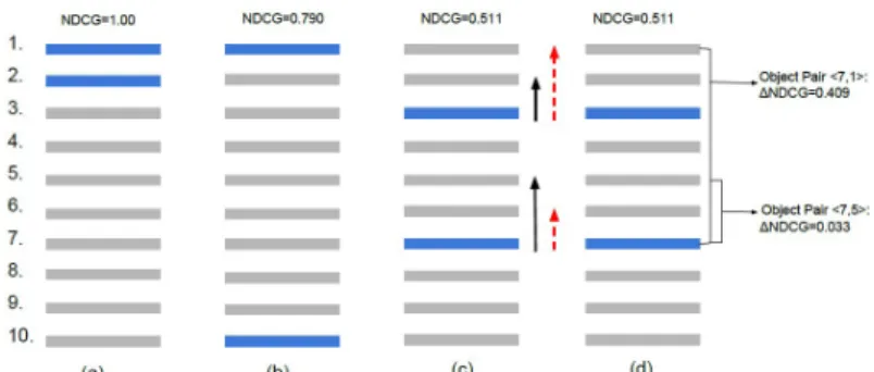
Figure 1: A set of items ordered for a given user using a binary relevance measure. The blue bars represent the items preferred by the user, while the light gray bars are those not preferred by the user. (a) is the ideal ranking; (b) is a ranking with eight pairwise errors; (c) and (d) are a ranking with seven pairwise errors by moving the top items of (b) down two rank levels, and the bottom preferred items up three. The two arrows (black solid and red dashed) of (c) denote two ways to minimize the pairwise er-rors. (d) shows the change in NDCG by swapping the orders of two items (e.g., item 7and item1).

3.2

Lambda Motivation

Top-N item recommendation is often referred to as a rank-ing task, where rankrank-ing measures like Normalized Discounted Cumulative Gain (NDCG) are widely adopted to evaluate the recommendation accuracy. However, it has been pointed out in previous IR literature (e.g., [19]) that pairwise loss functions might not match well with these measures. For easy reading, we start to state the problem by an intuitive example in the form of implicit feedback.

Figure 1 is a schematic that illustrates the relations of pairwise loss and NDCG. By comparison of (b) and (c), we observe two mismatch between them. First, the pairwise errors decrease from eight (b) to seven (c), along with the value of NDCG decreasing from 0.790 to 0.511. However, an ideal recommender model is supposed to increase the NDCG value with the drop of pairwise errors. Second, in (c), the arrows denote the next optimization direction and strength, and thus can be regarded as the gradients of PRFM. Al-though both arrows reduce the same amount of pairwise errors (i.e., three), the red dashed arrows lead to more gains as desired. This is because the new NDCGs, after the op-timization, are 0.624 and 0.832 by the black solid and red dashed arrows, respectively.

According to the above counterexamples, we clearly see that the pairwise loss function used in the optimization pro-cess is not a desired one as reducing its value does not neces-sarily increase the ranking performance. This means, PRFM might still be a suboptimal scheme for top-N recommenda-tions. This motivates us to study whether PRFM can be improved by concentrating on maximizing the ranking mea-sures.

To overcome the above challenge, Lambda-based meth-ods [19] in the field of IR have been proposed by directly optimizing the ranking biased performance measures. In-heriting the idea of LambdaRank, we design a new recom-mendation model named Lambda Factorization Machines (LambdaFM), an extended version of PRFM for solving top-N context-aware recommendations in implicit feedback do-mains. Following this idea, we can design a similar lambda

function asf(λi,j, ζu), whereζuis the current item ranking

list for user u (under context c). With NDCG as target,

f(λi,j, ζu) is given

f(λi,j, ζu) =λi,j|4N DCGij| (11)

where 4N DCGij is the NDCG difference of the ranking

list for a specific user if the positions (ranks) of itemsi, j

get switched. LambdaFM can be implemented by replacing

λi,j withf(λi,j, ζu) in Eqs. (9) and (10)3.

We find that the above implementation is reasonable for multi-label learning tasks in typical IR tasks, but not ap-plicable into IFCAR settings. This is because to calculate

4N DCGijit requires to compute scores of all items to

ob-tain the rankings of itemiandj. For the traditional LtR, the candidate URLs returned for a given query in train-ing datasets have usually been limited to a small size [31]. However, for recommendation, since there is no query at all, all unobserved (non-positive) items should be regarded as candidates, which leads to a very large size of candidates (see the items column in Table 1). Thus the complexity to calculate each training pair in IFCAR settings becomes

O(|I| ·Tpred), whereTpredis the time for predicting a score

by Eq. (3). That is, the original lambda function devised for LambdaRank is impractical for our settings.

4.

LAMBDA STRATEGIES

To handle the above problem, we need to revisit Eqs. (11), from which4N DCGijcan be interpreted as a weight

func-tion that it rewards a training pair by raising the learn-ing weight (i.e., λi,j) if the difference of NDCG is larger

after swapping the two items, otherwise it penalizes the training pair by shrinking the learning weight. Suppose an ideal lambda functionf(λi,j, ζu) for each training pair

hi, jiu is given with the current item ranking listζu, if we

design a scheme that generates the training item pairhi, jiu

with the probability proportional tof(λi,j, ζu)/λi,j(just like

4N DCGij in Eqs. (11)), then we are able to construct an

almost equivalent training model. In other words, a higher proportion of item pairs should be drawn according to the probability distributionpj ∝f(λi,j, ζu)/λi,j if they have a

larger4N DCGby swapping.

On the other hand, we observe that item pairs with a larger4N DCGcontribute more to the desired loss and lead to a larger NDCG value. In the following, we refer to a train-ing pair hi, jiu as an informative item pair, if 4N DCGij

is larger after swapping i and j than another pair hi, j0i. The unobserved itemjis called a good or informative item. Thus two research questions arise: (1) how to judge which item pairs are more informative? and (2) how to pick up informative items? Figure 1 (d) gives an example of which item pairs should have a higher weight. Obviously, we ob-serve that the quantity of4N DCG71 is larger than that of

4N DCG75. This indicates4N DCGijis likely to be larger

if unobserved (e.g., unselected) items have a higher rank (or a relatively higher score by Eq. (3)). This is intuitively cor-rect as the high ranked non-positive items hurt the ranking performance (users’ feelings) more than the low ranked ones. The other side of the intuition is that low ranked positive items contribute similarly as high ranked non-positive items during the training process, which would be provided with more details later.

3

Due to space limitations, we leave out more details and refer the interested readers to [29, 19] for the technical part.

In the following, we provide three intuitive lambda sur-rogates for addressing the two research questions and refer to PRFM with suggested lambda surrogates as LambdaFM (LFM for short in some places).

4.1

Static & Context-independent Sampler

We believe that a popular itemj ∈ I\Iuis supposed to

be a reasonable substitute for a high ranked non-positive item, i.e., the so-called informative item. The reason is in-tuitive as an ideal learning algorithm is expected to restore the pairwise ordering relations and rank most positive items with larger ranking scores than non-positive ones. As we know, the more popular an item is, the more times it acts as a positive one. Besides, popular items are more likely to be suggested by a recommender in general, and thus they have higher chances to be positive items. That is, the observa-tion that a user prefers an item over a popular one provides more information to capture her potential interest than that she prefers an item over a very unpopular one. Thus, it is reasonable to assign a higher weight to non-positive items with high popularity, or sampling such items with a higher probability.

In fact, it has been recognized that item popularity dis-tribution in most real-world recommendation datasets has a heavy tail [17, 13], following an approximate power-law or exponential distribution4_{. Accordingly, most non-positive}

items drawn by uniform sampling in Algorithm 1 are un-popular due to the long tail distribution, and thus contribute less to the desired loss function. Based on the analysis, it is reasonable to present a popularity-aware sampler to replace the uniform one before performing each SGD. Letpjdenote

the sampling distribution for itemj. In this work, we draw unobserved items with the probability proportional to the empirical popularity distribution, e.g., an exponential dis-tribution (In practice, the disdis-tribution pj can be replaced

with other analytic distributions, such as geometric and lin-ear distributions, or non-parametric ones).

pj∝exp −r(j) + 1 |I| ×ρ , ρ∈(0,1] (12)

where r(j) represents the rank of item j among all items

I according to the overall popularity,ρis the parameter of the distribution. Therefore, Line 7 in Algorithm 1 can be directly replaced as the above sampler, i.e., Eq. (12). Here-after, we denote PRFM with the static popularity-aware sampler as LFM-S.

The proposed sampler has three important properties:

• Static. The sampling procedure is static, i.e., the

dis-tribution does not change during the training process.

• Context-Invariant. The item popularity is

indepen-dent of context information according to Eq. (12).

• Efficient. The sampling strategy does not increase the

computational complexity since the popularity distri-bution is static and thus can be calculated in advance.

4.2

Dynamic & Context-aware Sampler

The second sampler is a dynamic one which is able to change the sampling procedure while the model parameters Θ are updated. The main difference of dynamic sampling is that the item rank is computed by their scores instead of global popularity. As it is computationally expensive to

4

We have examined the long tail property of our example datasets, while details are omitted for space reasons.

Algorithm 2Rank-Aware Dynamic Sampling

1: Require: Unobserved item setI\Iu, scoring function ˆy(·), parameterm, ρ

2: Draw samplej1,...,jmuniformly fromI\Iu

3: Compute ˆy(xj1_),...,ˆy(xjm₎

4: Sortj1,...,jmby descending order, i.e.,r(jm)∝ _yˆ(x1jm)

5: Return one item from the sorted list with the exponential distributionpj∝exp(−(r(j) + 1)/(m×ρ)).

calculate all item scores in the item list given a user and context, which is different from the static item popularity calculated in advance, we first perform a uniform sampling to obtain m candidates. Then we calculate the candidate scores and sample the candidates also by an exponential distribution. As the first sampling is uniform, the sampling probability density for each item is equivalent with that from the original (costy) global sampling. A straightforward al-gorithm can be implemented by Alal-gorithm 2. We denote PRFM with the dynamic sampler as LFM-D. It can be seen the sampling procedure is dynamic and context-aware.

• The sampler selects non-positive items dynamically ac-cording to the current item ranks which are likely to be different at each update.

• The item rank is computed by the FM function (i.e., Eq. (3)), which is clearly context-aware.

• The complexity for parameter update of each training pair is O(mTpred (Line 3)+mlogm (Line 4)), where

the number of sampling itemsmcan be set to a small value (e.g., m=10, 20, 50). Thus introducing the dy-namic sampler will not increase the time complexity much.

4.3

Rank-aware Weighted Approximation

The above two surrogates are essentially based on non-positive item sampling techniques, the core idea is to push non-positive items with higher ranks down from the top po-sitions. Based on the same intuition, an equivalent way is to pull positive items with lower ranks up from the bot-tom positions. That is, we have to place less emphasis on the highly ranked positives and more emphasis on the lowly ranked ones. Specifically, if a positive item is ranked top in the list, then we use a reweighting term Γ r(i)

to assign a smaller weight to the learning weightλi,j such that it will

not cost the loss too much. However, if a positive item is not ranked at top positions, Γ r(i)

will assign a larger weight to the gradient, pushing the positive item to the top.

f(λi,j, ζu) = Γ r(i)

λi,j (13)

By considering maximizing objectives e.g., reciprocal rank, we define Γ r(i) as Γ r(i) = 1 Γ I r(i) X r=0 1 r+ 1 (14) where Γ I

is the normalization term calculated by the the-oretically lowest position of a positive item, i.e.,

Γ I

=X r∈I

1

r+ 1 (15)

However, the same issue occurs again, i.e., the rank of the positive itemiis unknown without computing the scores of all items. In contrast with non-positive item sampling meth-ods, sampling positives is clearly useless as there are only a

Algorithm 3LFM-W Learning

1: Input:Training dataset, regularization parametersγ, learn-ing rateη

2: Output:Parameters Θ = (w,V)

3: Initialize Θ:w←(0, ...,0);V ∼ N(0,0.1);

4: repeat

5: Uniformly drawufromU

6: Uniformly drawifromIu

7: Calculate ˆy(xi)

8: SetT=0

9: do

10: Uniformly drawjfromI

11: Calculate ˆy(xj₎ 12: T+=1 13: while yˆ(xi_)−yˆ(xj_{)> εkP}u ij6= 1 ∧ T <|I| −1 14: ifyˆ(xi_)−yˆ(xj_)≤ε∧Pu ij= 1then

15: Calculateλi,j,Γ Iaccording to Eqs. (7) and (15)

16: fork∈ {1, ..., n} ∧xk6= 0 do 17: Updatewk: 18: wk←wk−η λi,j(xik−x j k) Pd |I|−1 T e r=0 r+11 ΓI −γwkwk 19: end for 20: forf∈ {1, ..., d}do 21: fork∈ {1, ..., n} ∧xk6= 0 do 22: Updatevk,f: 23: vk,f←vk,f−η λi,j Pnl=1vl,f(xikx i l−x j kx j l) −vk,f(xik 2 −xj_k2) Pd |I|−1 T e r=0 r+11 Γ I −γvk,fvk,f 24: end for 25: end for 26: end if 27: untilconvergence 28: return Θ

small fraction of positive items (i.e., |Iu|), and thus all of

them should be utilized to alleviate the sparsity. Interest-ingly, we observe that it is possible to compute the approx-imate rank of positive item iby sampling one incorrectly-ranked item. More specifically, given a hu, ii pair, we re-peatedly draw an item fromIuntil we obtain an incorrectly-ranked itemjsuch that ˆy(xi)−yˆ(xj)≤εandPuij=1, where

εis a positive margin value5_{. Let}

T denote the size of sam-pling trials before obtaining such an item. Apparently, the sampling process corresponds to a geometric distribution with parameter p = _|I|−r(i)₁. Since the number of sampling trials can be regarded as the expectation of parameterp, we have T ≈ d1

pe =d |I|−1

r(i) e, where d·eis the ceiling function.

Our idea here is similar to that used in [27, 28] for a dif-ferent problem. Finally, by using the estimation, we rewrite the gradient ∂L(hi, jiu) ∂θ = Pd |I|−1 T e r=0 1 r+1 Γ I λi,j ∂ˆy(xi₎ ∂θ − ∂yˆ(xj₎ ∂θ (16)

We denote the proposed algorithm based weighted approx-imation as LFM-W in Algorithm 3. In this algorithm, we iterate through all positive items i∈Iu for each user and

update the model parametersw,V until the procedure con-verges. In each iteration, given a user-item pair, the sam-pling process is first performed so as to estimate violating

5

We hypothesize that itemjis ranked higher thanifor useruonly if ˆy(xi)−y(ˆxj)≤ε, the default value ofεin this paper is set to 1.

condition and obtain a desired itemj6_{. Oncejis chosen, we}

update the model parameters by applying the SGD method. We are interested in investigating whether the weight ap-proximation yields the right contribution for the desired ranking loss. Based on Eq. (16), it is easy to achieve a potential loss induced by the violation ofhi, jiu pair using

back-stepping approach L hi, jiu= Pd |I|−1 T e r=0 1 r+1 Γ (I) log 1+exp −σ yˆ(xi)−ˆy(xj) (17)

To simplify the function, we first omit the denominator term since it is a constant value, then we replace the CE loss with the 0/1 loss function.

∂L(hi, jiu) ∂θ = r(i) X r=0 1 r+ 1I h ˆ y(xi)−yˆ(xj)i (18)

whereI[·] is the indicator function,I[h] = 1 whenhis true, and 0 otherwise. Thus, we haveI

ˆ

y(xi)−yˆ(xj

= 1 in all the cases becauseris smaller thanr(i). Moreover, for each positive itemi, there arer(i) items that are ranked higher thani(i.e., itemj), and thus eachjhas the probability of

p= 1

r(i) to be picked. Finally, the formulation of the loss

for each useruis simplified as7

Lu= X i∈Iu r(i) X r=0 1 r+ 1 (19)

As previously demonstrated in Section 3.2, the difference of pairwise losses between (b) and (c) in Figure 1 is inconsis-tent with that of NDCG values. Instead of using standard pairwise loss function, here we compute the losses based on Eq. (19), from which we achieve the losses of (b) and (c) are 2.93 and 4.43, respectively. This means, a smaller loss leads to a larger NDCG value, and vice versa. Similarly, we no-tice that the black (solid) arrows in (c) after movement lead to a larger loss than the red (dashed) ones, and in reason, the new NDCG value generated by the black ones is smaller than that by the red ones. Therefore, the movement direc-tion and strength of red arrows is the right way to minimize a larger loss, which also demonstrates the correctness of the proposed lambda strategy. Based on Eq. (19), one can draw similar conclusions using other examples.

Regarding the properties of LFM-W, we observe that the weight approximation procedure is both dynamic (Line 9-13 of Algorithm 3) and context-aware (Line 11) during each update, similarly like LFM-D. Moreover, LFM-W is able to leverage both binary and graded relevance datasets (e.g. URL click numbers, POI check-ins), whereas LFM-S and LFM-D cannot learn the count information from positives. In terms of the computational complexity, using the gradient calculation in Eq. (16) can achieve important speedups. The complexity to compute 4N DCG is O(Tpred|I|) while the

complexity with weighted approximation becomesO(TpredT).

Generally, we haveT |I|at the start of the training and

T <|I|when the training reaches a stable state. The reason

is that at the beginning, LambdaFM is not well trained and thus it is quick to find an offending itemj, which leads to a very smallT, i.e., T |I|, when the training converges to a stable state, most positive items are likely to be ranked correctly, which is also our expectation, and thusT becomes a bit larger. However, it is unlikely that all positive items are ranked correctly, so in general we haveT <|I|.

6

Itemj is not limited to a non-positive item, since it can also be drawn from the positive collectionIuwith a lower preference thani.

7

Please note thatLu is non-continuous and indifferentiable, which

means it is hard to be directly optimized with this form.

5.

LAMBDA WITH ALTERNATIVE LOSSES

From Section 3.1, one may observe that the original lambda function was a specific proposal for the CE loss function used in RankNet [2]. To our knowledge, there exists a large class of pairwise loss functions in IR literature. The well-known pairwise loss functions, for example, can be margin ranking criterion, fidelity loss, exponential loss, and modified Huber loss, which are used in Ranking SVM [9], Frank [15], Rank-Boost [7], quadratically smoothed SVM [30], respectively. Motivated by the design ideas of these famous algorithms, we build a family of LambdaFM variants based on these loss functions and verify the generic properties of our lambda surrogates.

Margin ranking criterion(MRC):

L=X u∈U X i∈Iu X j∈I\I_u max0,1−(ˆy(xi)−yˆ(xj)) (20) MRC assigns each positive-negative (non-positive) item pair a cost if the score of non-positive item is larger or within a margin of 1 from the positive score. Optimizing this loss is equivalent to maximizing the area under the ROC curve (AUC). Since MRC is non-differentiable, we optimize its subgradient as follows

λi,j=

−1 if ˆy(xi_)−yˆ(xj_)<1

0 if ˆy(xi_)−yˆ(xj_)≥1 (21)

As is known, the pairwise violations are independent of their positions in the ranking list [10]. For this reason, MRC might not optimize top-N very accurately.

Fidelity loss (FL): This loss is introduced by Tsai et al. [15] and has been applied in Information Retrieval (IR) task and yielded superior performance. The original func-tion regarding the loss of pairs is defined as

L=X u∈U X i∈I X j∈I 1− q Pij·Pi,j− q (1−Pij)·(1−Pi,j) (22)

where Pij and Pij share the same meanings with the CE

loss in Eq. (1). According to the antisymmetry of pairwise ordering scheme [23], we simplify the FL in IFCAR settings as follows L= X u∈U X i∈Iu X j∈I\Iu 1−q 1 1 + exp −ˆy(xi_{) + ˆy(x}j₎ (23)

In contrast with other losses (e.g., the CE and exponential losses), the FL of a pair is bounded between 0 and 1, which means the model trained by it is more robust against the influence of hard pairs. However, we argue that (1) FL is non-convex, which makes it difficult to optimize; (2) adding bound may cause insufficient penalties of informative pairs.

Modified Huber loss(MHL):

L= X u∈U X i∈Iu X j∈I\I_u 1 2γmax 0,1− ˆy(xi)−yˆ(xj) 2 (24)

where γ is a positive constant and is set to 2 for evalua-tion [30]. MHL is quadratically smoothed variant of MRC and proposed for linear prediction problems by Zhang et al. [30].

It is worth noting that both Fidelity and Huber loss func-tions have not been investigated yet in the context of recom-mendation. Besides, to the best of our knowledge, PRFM built on these two loss functions are novel. On the other hand, we find that exponential loss function is aggressive

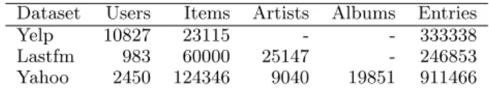
Table 1: Basic statistics of datasets. Each entry indicates whether a user has interacted with an item.

Dataset Users Items Artists Albums Entries Yelp 10827 23115 - - 333338 Lastfm 983 60000 25147 - 246853 Yahoo 2450 124346 9040 19851 911466

and seriously biased by hard pairs, which usually result in worse performance during the experiment. Thus the trial of PRFM with exponential loss have been omitted.

6.

EXPERIMENTS

In this section, we conduct experiments on the three real-world datasets to verify the effectiveness of our proposed LambdaFM in various settings.

6.1

Experimental Setup

6.1.1

Datasets & Evaluation Metrics

We use three publicly accessible Collaborative Filtering (CF) datasets for our experiments: Yelp8_{(user-venue pairs),}

Lastfm9_{(user-music-artist triples) and Yahoo music}10

(user-music-artist-album tuples). To speed up the experiments, we follow the same procedures as in [5, 16] by randomly sam-pling a subset of users from the user pool of Yahoo datasets, and a subset of items from the item pool of Lastfm dataset. On Yelp dataset, we extract data from Phoenix and follow the common practice [23] to filter out users with less than 10 interactions. The reason is because the original Yelp dataset is much sparser than Lastfm and Yahoo datasets11_{, which}

makes it difficult to evaluate recommendation algorithms (e.g., over half users have only one entry.). The statistics of the datasets after preprocessing are summarized in Table 1. To illustrate the recommendation quality of LambdaFM, we adopt four standard ranking metrics: Precision@N and Recall@N (denoted by Pre@N and Rec@N respectively) [12], Normalized Discounted Cumulative Gain (NDCG) [16, 14] and Mean Reciprocal Rank (MRR) [26], and one (binary) classification metric, i.e. Area Under ROC Curve (AUC). For each evaluation metric, we first calculate the perfor-mance of each user from the testing set, and then obtain the average performance over all users. Due to the page limita-tions, we leave out the detailed formulas of these measures.

6.1.2

Baseline Methods

In our experiments, we compare our model with five pow-erful baseline methods12_{. Most Popular (MP)[16, 23]:}

It is to recommend users with the top-N most popular items.

User-based Collaborative Filtering (UCF)[8, 23]: This is a typical memory-based CF technique for recommender systems. The preference quantity of useruto a candidate itemiis calculated as an aggregation of some similar users’ preference on this item. Pearson correlation is used in our work to compute user similarity and the top-30 most similar users are selected as the nearest neighbors. Factorization Machines (FM)[20, 21]: FM is designed for the rating

8 https://www.yelp.co.uk/dataset challenge 9 http://www.dtic.upf.edu/˜ocelma/MusicRecommendationDataset/ lastfm-1K.html 10_{webscope.sandbox.yahoo.com/catalog.php?datatype=r&did=2} 11

Cold users of both datasets have been trimmed by official provider.

12

For the sake of understanding the ranking effectiveness of different algorithms, we launch a random one (denoted as Rand) as in [8].

prediction task (known as a pointwise approach). Here we adapt FM for the item recommendation task by binariz-ing the ratbinariz-ing value. Note that, to conduct a fair compar-ison, we also develop the bootstrap sampling to make use of non-positive items, which outperforms FM in libFM [21].

Bayesian Personalized Ranking (BPR) [23]: This is one of the strongest context-free recommendation algorithms specifically designed for top-N item recommendations based on implicit feedback. Pairwise Ranking Factorization Machines (PRFM) [18]: To the best of our knowledge, PRFM is the state-of-the-art context-aware ranking algo-rithm, optimized to maximize the AUC metric. In this pa-per, we develop several PRFM13_{algorithms by applying}

var-ious pairwise loss functions introduced in Section 5.

6.1.3

Hyper-parameter Settings

Learning rate η: We apply the 5-fold cross validation to find η for PRFM14_{, and then employ the same η to}

LambdaFM for comparison. In addition, for BPR, the ex-perimental results show that it performs the best with the same set of parameters of PRFM; for FM, we apply the same procedure to choseηindependently. Latent dimensiond: The effect of latent factors has been well studied by previous work, e.g., [23]. For comparison purposes, the approaches (e.g., [16]) are usually to assign a fixeddvalue (e.g.,d= 30 in our experiments) for all methods based on factorization models. Regularization γθ: LambdaFM has several

regu-larization parameters, includingγwk,γvk,f, which represent

the regularization parameters of latent factor vectors ofwk,

vk,f, respectively. We borrow the idea from [21] by grouping

them for each factor layer, i.e., γπ =γwk,γξ =γvk,f. We

run LambdaFM withγπ, γξ ∈ {0.5,0.1,0.05,0.01,0.005}to

find the best performance parameters. Distribution co-efficient ρ: ρ ∈ (0,1] is specific for LFM-S and LFM-D, which is usually tuned according to the data distribution.

6.2

Performance Evaluation

All experiments are conducted with the standard 5-fold cross validation. The average results over 5 folds are re-ported as the final performance.

6.2.1

Accuracy Summary

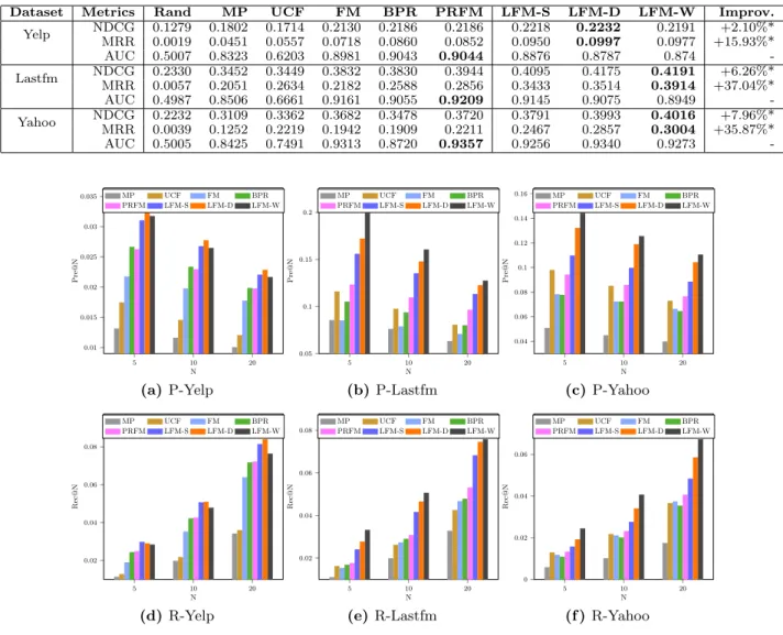
Table 2 and Figure 2(a-f) show the performance of all the methods on the three datasets. Several insightful ob-servations can be made: First, in most cases personalized models (UCF, BPR, PRFM, LambdaFM) noticeably out-perform MP, which is a non-personalized method. This im-plies, in practice, when there is personalized information present, personalized recommenders are supposed to outper-form non-personalized ones. Particularly, our LambdaFM clearly outperforms all the counterparts in terms of four ranking metrics. Second, we observe that different mod-els yield basically consistent recommendation accuracy on different metrics, except for AUC, which we give more de-tails later. Third, as N increases, values of Pre@N get lower and values of Rec@N become higher. The trends reveal the typical behavior of recommender systems: the more items are recommended, the better the recall but the worse the precision achieved.

Regarding the effectiveness of factorization models, we find that BPR performs better than FM on the Yelp dataset15_, 13_{PRFM is short for PRFM with the CE loss if not explicitly declared.} 14

ηis set to 0.01 on Yelp and Yahoo datasets, and 0.08 on Lastfm.

15

Note that it is not comparable on the Lastfm and Yahoo datasets since FM combines other contexts.

Table 2: Performance comparison on NDCG, MRR and AUC, where “*” means significant improvement in terms of paired t-test with p-value<0.01. For each measure, the best result is indicted in bold.

Dataset Metrics Rand MP UCF FM BPR PRFM LFM-S LFM-D LFM-W Improv. Yelp NDCG 0.1279 0.1802 0.1714 0.2130 0.2186 0.2186 0.2218 0.2232 0.2191 +2.10%* MRR 0.0019 0.0451 0.0557 0.0718 0.0860 0.0852 0.0950 0.0997 0.0977 +15.93%* AUC 0.5007 0.8323 0.6203 0.8981 0.9043 0.9044 0.8876 0.8787 0.874 -Lastfm NDCG_MRR 0.2330_0.0057 0.3452_0.2051 0.3449_{0.2634 0.2182}0.3832 _0.25880.3830 _0.28560.3944 _0.34330.4095 _0.35140.4175 _0.39140.4191 _+37.04%*+6.26%* AUC 0.4987 0.8506 0.6661 0.9161 0.9055 0.9209 0.9145 0.9075 0.8949 -Yahoo NDCG_MRR 0.2232_0.0039 0.3109_0.1252 0.3362_{0.2219 0.1942}0.3682 _0.19090.3478 _0.22110.3720 _0.24670.3791 _0.28570.3993 _0.30040.4016 _+35.87%*+7.96%* AUC 0.5005 0.8425 0.7491 0.9313 0.8720 0.9357 0.9256 0.9340 0.9273 -5 10 20 0.01 0.015 0.02 0.025 0.03 0.035 N Pre@N MP UCF FM BPR PRFM LFM-S LFM-D LFM-W (a) P-Yelp 5 10 20 0.05 0.1 0.15 0.2 N Pre@N MP UCF FM BPR PRFM LFM-S LFM-D LFM-W (b)P-Lastfm 5 10 20 0.04 0.06 0.08 0.1 0.12 0.14 0.16 N Pre@N MP UCF FM BPR PRFM LFM-S LFM-D LFM-W (c)P-Yahoo 5 10 20 0.02 0.04 0.06 0.08 N Rec@N MP UCF FM BPR PRFM LFM-S LFM-D LFM-W (d) R-Yelp 5 10 20 0.02 0.04 0.06 0.08 N Rec@N MP UCF FM BPR PRFM LFM-S LFM-D LFM-W (e)R-Lastfm 5 10 20 0 0.02 0.04 0.06 N Rec@N MP UCF FM BPR PRFM LFM-S LFM-D LFM-W (f )R-Yahoo

Figure 2: Performance comparison with respect to top-N values, i.e., Pre@N (P) and Rec@N (R).

0.01 0.1 0.3 0.5 0.8 1.0 0.01 0.03 0.05 0.07 0.09 ρ MRR PRFM LFM-S LFM-D LFM-W (a)Yelp 0.01 0.1 0.3 0.5 0.8 1.0 0.24 0.28 0.32 0.36 0.4 ρ MRR PRFM LFM-S LFM-D LFM-W (b)Lastfm 0.01 0.1 0.3 0.5 0.8 1.0 0.05 0.1 0.15 0.2 0.25 0.3 ρ MRR PRFM LFM-S LFM-D LFM-W (c) Yahoo

Figure 3: Parameter tuning with respect to MRR.

which empirically implies pairwise methods outperform point-wise ones for ranking tasks. The reason is that FM is identi-cal to matrix factorization with only user-item information. In this case, the main difference of FM and BPR is that they apply different loss functions, i.e., quadratic and logistic loss, respectively. This is in accordance with the interesting find-ing that BPR and PRFM produce nearly the same results

w.r.t. all metrics on Yelp. Furthermore, among all the base-line models, the performance of PRFM is very promising. The reason is that PRFM, (1) as a ranking-based factoriza-tion method, is more appropriate for handling top-N item recommendation tasks (vs. FM); (2) by applying FM as scoring function, PRFM estimates more accurate ordering relations than BPR due to auxiliary contextual variables.

(u, i) (u, i, a) 0.2 0.25 0.3 0.35 0.4 Context MRR PRFM LFM-S LFM-D LFM-W (a) Lastfm

(u, i) (u, i, a) (u, i, a, a) 0.18 0.2 0.22 0.24 0.26 0.28 0.3 Context MRR PRFM LFM-S LFM-D LFM-W (b)Yahoo

Figure 4: Performance comparison in terms of MRR with different context.

LFM vs. PRFM:We observe that in Figure 2 and Table 2 our LambdaFM (including LFM-S, LFM-D and LFM-W) consistently outperforms the state-of-the-art method PRFM in terms of four ranking metrics. In particular, the improve-ments on Lastfm and Yahoo datasets w.r.t. NDCG and MRR, are more than 6% and 35%, respectively. Similar improvements w.r.t. Pre@N and Rec@N metrics can be ob-served from Figure 216_{. Besides, we observe that LFM}

un-derperforms PRFM in terms of AUC. The results validate our previous analysis, namely, LambdaFM is trained to op-timize ranking measures while PRFM aims to maximize the AUC metric. This indicates that pairwise ranking models, such as BPR and PRFM, may not be good approximators of the ranking biased metrics and such a mismatch empirically leads to non-optimal ranking.

6.2.2

Effect of Lambda Surrogates

In this subsection, we study the effect of lambda surro-gates and parameter influence on the recommendation per-formance. For LFM-S, we directly tune the value ofρ; for LFM-D, we fix the number of sampling units m to a con-stant, e.g., m= 10, and then tune the value ofρ ∈ {0.01, 0.1, 0.3, 0.5, 0.8, 1.0}; and for LFM-W the only parameter

ε is fixed at 1 for all three datasets in this work. Figure 3 depicts the performance changes by tuningρ. First, we see LFM-W performs noticeably better than PRFM, and by choosing a suitableρ(e.g., 0.3 for S and 0.1 for LFM-D), both LFM-D and LFM-S also perform largely better than PRFM. This indicates the three suggested lambda sur-rogates work effectively for handling the mismatch drawback between PRFM and ranking measures. Second, LFM-S pro-duces best accuracy when settingρto 0.3 on all datasets but the performance experiences a significant decrease when set-tingρto 0.1. The reason is that the SGD learner will make more gradient steps on popular items due to the oversam-pling whenρis set too small according to Eq. (12). In this case, most less popular items will not be picked for training, and thus the model is under-trained. By contrast, the per-formance of LFM-D has not dropped on Yahoo dataset even whenρis set to 0.01 (which means picking the top fromm

randomly selected items, see Algorithm 2). This implies, the performance may be further improved by setting a largerm. Third, the results indicate that LFM-D and LFM-W outper-form LFM-S on Lastfm and Yahoo datasets17_{. This is} be-16

To save space, we only use MRR for the following discussion since the performance trend on other ranking metrics is consistent.

17

The superiority is not obvious on the Yelp dataset. This might be due to the reason that the Yelp dataset has no additional context and the item tail is relatively shorter than that of other datasets.

cause the static sampling method ignores the fact that the estimated ranking of a non-positive item j changes during learning, i.e., j might be ranked high in the first step but it is ranked low after several iterations18_{. Besides, LFM-S}

computes the item ranking based on the overall popularity, which does not reflect the context information. Thus, it is more encouraged to exploit current context for computing ranking such as LFM-D and LFM-W.

6.2.3

Effect of Context

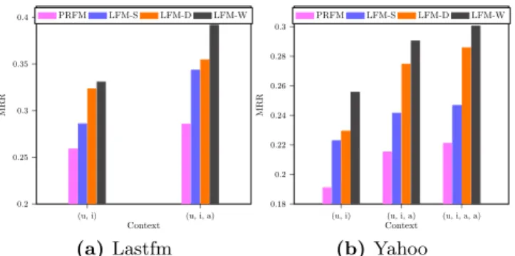
Finding competitive contextual features is not the main focus of this work but it is interesting to see to what ex-tent LambdaFM improves the performance by adding con-text. Therefore, we conduct a contrast experimentation and show the results on Figure 4(a-b)19_{, where (}

u, i) denotes a user-item (i.e., music) pair and (u, i, a) denotes a user-item-artist triple on both datasets; similarly, (u, i, a, a) represents a user-item-artist-album quad on Yahoo dataset. First, we observe LambdaFM performs much better with (u, i, a) tu-ples than that with (u, i) tuples on both datasets. This result is consistent with the intuition that a user may like a song if she likes another song by the same artist. Second, as expected, LambdaFM with (u, i, a, a) tuples performs fur-ther better than that with (u, i, a) tuples from Figure 4(b). We draw the conclusion that, by inheriting the advantage of FM, the more effective context incorporated, the better LambdaFM performs.

6.2.4

Lambda with Alternative Loss Functions

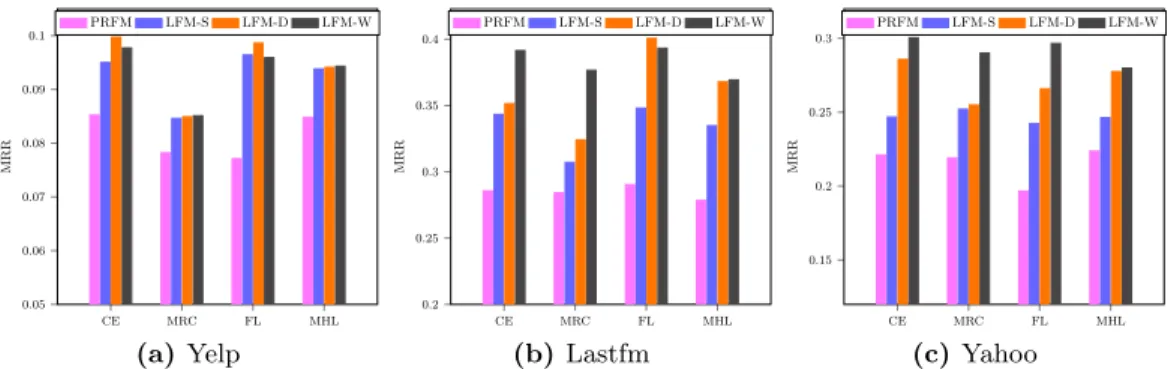
Following the implementations of well-known pairwise LtR approaches introduced in Section 5, we have built a family of PRFM and LambdaFM variants. Figure 5 shows the per-formance of all these variants based on corresponding loss functions. Based on the results, we observe that by imple-menting the lambda surrogates, all variants of LambdaFM outperform PRFM, indicating the generic properties of these surrogates. Among the three lambda surrogates, the perfor-mance trends are in accordance with previous analysis, i.e. LFM-W and LFM-D perform better than LFM-S. Addition-ally, most recent literature using pairwise LtR for recom-mendation is based on BPR optimization criterion, which is equivalent to the CE loss in the implicit feedback scenarios. To the best of our knowledge, the performance of FL and MHL loss functions have not been investigated in the con-text of recommendation, and also PRFM and LambdaFM based on FL and MHL loss functions achieve competitive performance with the ones using the CE loss. We expect our suggested PRFM (with new loss functions) and LambdaFM to be valuable for existing recommender systems that are based on pairwise LtR approaches.

7.

CONCLUSION AND FUTURE WORK

In this paper, we have presented a novel ranking predic-tor Lambda Facpredic-torization Machines (LambdaFM). Inherit-ing advantages from both LtR and FM, LambdaFM (i) is capable of optimizing various top-N item ranking metrics in implicit feedback settings; (ii) is very flexible to incor-porate context information for context-aware recommenda-tions. Different from the original lambda strategy, which is tailored for the CE loss function, we have proved that our proposed lambda surrogates are more general and applicable

18

In spite of this, non-positive items drawn by popularity sampler are still more informative than those drawn by uniform sampler.

19

ρis assigned a fixed value for the study of context effect, namely 0.1 and 0.3 for LFM-D and LFM-S, respectively.

CE MRC FL MHL 0.05 0.06 0.07 0.08 0.09 0.1 MRR PRFM LFM-S LFM-D LFM-W (a) Yelp CE MRC FL MHL 0.2 0.25 0.3 0.35 0.4 MRR PRFM LFM-S LFM-D LFM-W (b)Lastfm CE MRC FL MHL 0.15 0.2 0.25 0.3 MRR PRFM LFM-S LFM-D LFM-W (c)Yahoo

Figure 5: The variants of PRFM and LambdaFM based on various pairwise loss functions.

to a set of well-known ranking loss functions. Furthermore, we have built a family of PRFM and LambdaFM algorithms, shedding light on how they perform in real tasks. In our eval-uation, we have shown that LambdaFM largely outperforms state-of-the-art counterparts in terms of four standard rank-ing measures, but underperforms PRFM methods in terms of AUC, known as a binary classification measure.

LambdaFM is also applicable to other important rank-ing tasks based on implicit feedback, e.g., personalized mi-croblog retrieval and learning to personalize query auto-completion. In future work, it would be interesting to inves-tigate its effectiveness in these scenarios.

8.

ACKNOWLEDGMENTS

Fajie thanks the CSC funding for supporting the research. This work is also supported by the National Natural Science Foundation of China under Grant No. 61402097.

9.

REFERENCES

[1] Baltrunas. Incarmusic: Context-aware music

recommendations in a car. InEC-Web, pages 89–100, 2011. [2] C. Burges, T. Shaked, E. Renshaw, A. Lazier, M. Deeds,

N. Hamilton, and G. Hullender. Learning to rank using gradient descent. InICML, pages 89–96, 2005.

[3] Z. Cao, T. Qin, T. Liu, M. Tsai, and H. Li. Learning to rank: from pairwise approach to listwise approach. In ICML, pages 129–136, 2007.

[4] T. Chen, W. Zhang, Q. Lu, K. Chen, Z. Zheng, and Y. Yu. Svdfeature: a toolkit for feature-based collaborative filtering.JMLR, pages 3619–3622, 2012.

[5] K. Christakopoulou and A. Banerjee. Collaborative ranking with a push at the top. InWWW, pages 205–215, 2015. [6] P. Cremonesi, Y. Koren, and R. Turrin. Performance of

recommender algorithms on top-n recommendation tasks. InRecSys, pages 39–46, 2010.

[7] Y. Freund, R. Iyer, R. E. Schapire, and Y. Singer. An efficient boosting algorithm for combining preferences. JMLR, pages 933–969, 2003.

[8] H. Gao, J. Tang, X. Hu, and H. Liu. Exploring temporal effects for location recommendation on location-based social networks. InRecSys, pages 93–100, 2013. [9] R. Herbrich, T. Graepel, and K. Obermayer. Support

vector learning for ordinal regression. 1999. [10] L. Hong, A. S. Doumith, and B. D. Davison.

Co-factorization machines: modeling user interests and predicting individual decisions in twitter. InWSDM, pages 557–566, 2013.

[11] A. Karatzoglou, X. Amatriain, L. Baltrunas, and N. Oliver. Multiverse recommendation: n-dimensional tensor

factorization for context-aware collaborative filtering. In RecSys, pages 79–86, 2010.

[12] X. Li, G. Cong, X.-L. Li, T.-A. N. Pham, and S. Krishnaswamy. Rank-geofm: a ranking based geographical factorization method for point of interest recommendation. InSIGIR, pages 433–442, 2015.

[13] Q. Lu, T. Chen, W. Zhang, D. Yang, and Y. Yu. Serendipitous personalized ranking for top-n recommendation. InWI-IAT, pages 258–265, 2012. [14] B. McFee and G. R. Lanckriet. Metric learning to rank. In

ICML, pages 775–782, 2010.

[15] M.Tsai, T.Liu, T.Qin, H.Chen, and W.Ma. Frank: a ranking method with fidelity loss. InSIGIR, pages 383–390, 2007.

[16] W. Pan and L. Chen. GBPR: Group preference based bayesian personalized ranking for one-class collaborative filtering. InIJCAI, pages 2691–2697, 2013.

[17] Y.-J. Park and A. Tuzhilin. The long tail of recommender systems and how to leverage it. InRecSys, pages 11–18, 2008.

[18] R. Qiang, F. Liang, and J. Yang. Exploiting ranking factorization machines for microblog retrieval. InCIKM, pages 1783–1788, 2013.

[19] C. Quoc and V. Le. Learning to rank with nonsmooth cost functions. 19:193–200, 2007.

[20] S. Rendle. Factorization machines. InICDM, pages 995–1000, 2010.

[21] S. Rendle. Factorization machines with libFM.TIST, pages 57:1–57:22, 2012.

[22] S. Rendle and C. Freudenthaler. Improving pairwise learning for item recommendation from implicit feedback. InWSDM, pages 273–282, 2014.

[23] S. Rendle, C. Freudenthaler, Z. Gantner, and

L. Schmidt-Thieme. BPR: bayesian personalized ranking from implicit feedback. InUAI, pages 452–461, 2009. [24] Y. Shi, A. Karatzoglou, L. Baltrunas, M. Larson, and

A. Hanjalic. Cars2: Learning context-aware representations for context-aware recommendations. InCIKM, pages 291–300, 2014.

[25] Y. Shi, A. Karatzoglou, L. Baltrunas, M. Larson, A. Hanjalic, and N. Oliver. TFMAP: optimizing map for top-n context-aware recommendation. InSIGIR, pages 155–164, 2012.

[26] Y. Shi, A. Karatzoglou, L. Baltrunas, M. Larson, N. Oliver, and A. Hanjalic. CLiMF: learning to maximize reciprocal rank with collaborative less-is-more filtering. InRecSys, pages 139–146, 2012.

[27] N. Usunier, D. Buffoni, and P. Gallinari. Ranking with ordered weighted pairwise classification. InICML, pages 1057–1064, 2009.

[28] J. Weston, S. Bengio, and N. Usunier. Wsabie: Scaling up to large vocabulary image annotation. InIJCAI, pages 2764–2770, 2011.

[29] F. Yuan, G. Guo, J. Jose, L. Chen, H. Yu, and W. Zhang. Optimizing factorization machines for top-n context-aware recommendations. InWISE, 2016.

[30] T. Zhang. Solving large scale linear prediction problems using stochastic gradient descent algorithms. InICML, page 116, 2004.

[31] W. Zhang, T. Chen, J. Wang, and Y. Yu. Optimizing top-n collaborative filtering via dynamic negative item sampling. InSIGIR, pages 785–788, 2013.