Large Scale Machine Learning in Biology

(1)

Anil Raj

Submitted in partial fulfillment of the requirements for the degree of

Doctor of Philosophy

in the Graduate School of Arts and Sciences

COLUMBIA UNIVERSITY

(2)

(3)

Large Scale Machine Learning in Biology

Anil Raj

Rapid technological advances during the last two decades have led to a data-driven rev-olution in biology opening up a plethora of opportunities to infer informative patterns that could lead to deeper biological understanding. Large volumes of data provided by such technologies, however, are not analyzable using hypothesis-driven significance tests and other cornerstones of orthodox statistics. We present powerful tools in machine learn-ing and statistical inference for extractlearn-ing biologically informative patterns and clinically predictive models using this data.

Motivated by an existing graph partitioning framework, we first derive relationships between optimizing the regularized min-cut cost function used in spectral clustering and the relevance information as defined in the Information Bottleneck method. For fast-mixing graphs, we show that the regularized min-cut cost functions introduced by Shi and Malik over a decade ago can be well approximated as the rate of loss of predictive information about the location of random walkers on the graph. For graphs drawn from a generative model designed to describe community structure, the optimal information-theoretic partition and the optimal min-cut partition are shown to be the same with high probability.

Next, we formulate the problem of identifying emerging viral pathogens and charac-terizing their transmission in terms of learning linear models that can predict the host of a virus using its sequence information. Motivated by an existing framework for represent-ing biological sequence information, we learn sparse, tree-structured models, built from decision rules based on subsequences, to predict viral hosts from protein sequence data using multi-class Adaboost, a powerful discriminative machine learning algorithm. Fur-thermore, the predictive motifs robustly selected by the learning algorithm are found to

(4)

We then extend this learning algorithm to the problem of predicting disease risk in hu-mans using single nucleotide polymorphisms (SNP) — single-base pair variations — in their entire genome. While genome-wide association studies usually aim to infer individ-ual SNPs that are strongly associated with disease, we use popular supervised learning algorithms to infer sufficiently complex tree-structured models, built from single-SNP de-cision rules, that are both highly predictive (for clinical goals) and facilitate biological in-terpretation (for basic science goals). In addition to high prediction accuracies, the models identify ‘hotspots’ in the genome that contain putative causal variants for the disease and also suggest combinatorial interactions that are relevant for the disease.

Finally, motivated by the insufficiency of quantifying biological interpretability in terms of model sparsity, we propose a hierarchical Bayesian model that infers hidden structured relationships between features while simultaneously regularizing the classification model using the inferred group structure. The appropriate hidden structure maximizes the log-probability of the observed data, thus regularizing a classifier while increasing its pre-dictive accuracy. We conclude by describing different extensions of this model that can be applied to various biological problems, specifically those described in this thesis, and enumerate promising directions for future research.

(5)

List of Figures

2.1 Min-cut of a network . . . 9

2.2 Comparison of the exact and approximate formulae for the Jensen Shannon Divergence. . . 19

2.3 Probability of numerical precision error when computing the Jensen Shan-non Divergence. . . 20

2.4 Quantifying the long-time and short-time approximations of the relevance information. . . 27

2.5 Scatter plot of minimum approximation error and normalized diffusion time for random graphs drawn from a Stochastic Block Model. . . 29

2.6 Scatter plot of minimum approximation error and diffusion time for ran-domly generated graphs. . . 30

2.7 Quantifying the agreement between min-cut solutions and those from max-imizing relevance information. . . 31

3.1 An example of an ADT . . . 39

3.2 Quantifying the accuracy of predicting hosts ofPicornaviridae . . . 44

3.3 Quantifying the accuracy of predicting hosts ofRhabdoviridae. . . 45

3.4 A visualization of the predictivek-mers forPicornaviridae . . . 46

3.5 A visualization of predictive “hotspots” of viral proteomes . . . 47

4.1 SNP log-intensity scatter plot . . . 59

4.2 Pathologies in genotype calling . . . 60

4.3 An example of a one-sided ADT. . . 63

(8)

4.5 Visual depiction of growing an ADT. . . 66

4.6 Receiver operating characteristic curve. . . 70

4.7 Quantifying the accuracy of different algorithms and models on T1D. . . 72

4.8 Quantifying the accuracy of different algorithms and models on T2D. . . 73

4.9 Quantifying the change of weights in ADT when using ERLPboost. . . 74

4.10 Quantifying the amount of predictive signal in the SNP data for different diseases. . . 75

4.11 Histogram of angles with the decision boundaries indicated for a SNP with a positively associated rare allele. . . 81

4.12 Histogram of angles with the decision boundaries indicated, for a SNP with a negatively associated rare allele. . . 82

4.13 Visual display of predictive “hotspots” for Type-1 diabetes. . . 83

4.14 Histogram of angles with the learned pathological decision boundaries in-dicated. . . 84

5.1 Example of a probabilistic graphical model. . . 91

5.2 Graphical model representing the Group Structured Classification Model. . 95

5.3 Illustrating the classification accuracy of GSCM. . . 99

5.4 Illustrating the clustering accuracy of GSCM. . . 100

5.5 Comparing the accuracy of GSCM with other structured-sparsity inducing classifiers. . . 102

(9)

List of Tables

3.1 Mismatch feature space . . . 37

A.1 List of viruses inRhabdoviridaefamily used in learning. . . 122 A.2 List of viruses inPicornaviridaefamily used in learning. . . 124

(10)

It is a great pleasure to acknowledge the many individuals who have encouraged, sup-ported, and contributed to the research presented here and, more generally, my overall education.

First, I would like to thank my advisor, Chris Wiggins, who has played an instrumental role in guiding my education and interests, and in opening up opportunities for me. Chris’ endless curiosity, immense patience, and ability to stay focused and “think in equations” as a scientist and mathematician are truly inspirational; I have learned more from him than I can possibly list here. His character and sense of humor have made this experience thoroughly enjoyable.

I would like to thank my family for making any of this possible: my parents Sasikala and Rajendran, for being the most influential teachers in my life and for ensuring that I enjoyed more opportunities than they were afforded; my brother Vimal and cousin Rajeev for their unconditional support and confidence; and my uncle Radhakrishnan for encour-aging my scientific curiosity and inspiring me to follow my passion for research.

I would like to thank my co-authors for their collaboration and numerous insights in our study characterizing virus host, including Mike Dewar, Gustavo Palacios and Raul Rabadan. I would also like to thank my collaborators Matan Hofree, Trey Ideker and Yoav Freund for providing the data and their excellent feedback in our study inferring genetic models for predicting disease. I am grateful to my dissertation committee, Adam Sobel, Chris Marianetti and David Madigan for their valuable time and attention in participating in my defense.

I also have the great pleasure of thanking my colleagues and friends: members of the Wiggins lab, including Mike Dewar, Jake Hofman, Andrew Mugler, Adrian Haimovich and Jonathan Bronson for the enlightening discussions, for teaching me the skills and sharing their wisdom necessary for graduate school and life after; and Yana Pleshivoy, Milena Zaharieva, Rebecca Plummer, Tatiana Pataria and Elena Norakidze for being ex-cellent friends and a source of support and inspiration.

Anil Raj New York, July 2011

(11)

(12)

Chapter 1

Introduction

Biology in the twentieth-century has primarily focused on discovering molecular changes and interactions amongst them underlying various observed biological phenomena. A prime example of this can be found in genetics where investigation of heritable variation in the early twentieth-century led to the discovery of discrete, heritable, functional compo-nents called genes, the discovery of DNA as the underlying molecule that encodes genetic information and the articulation of the central dogma of molecular biology — DNA en-codes for the structure and function of proteins whose synthesis and activity are regulated with the aid of intermediate molecules called RNA.

The traditional hypothesis-driven approach to this discovery process involves design-ing model systems that give rise to observed phenomena and makdesign-ing theoretical predic-tions using them. The key goal is to choose models complex enough for their predicpredic-tions to closely match the observables, yet simple enough to generalize to future observations and have a biological interpretation that is meaningful in the context of related phenomena and within the constraints of evolution. This process of discovery, however, has mostly been successful in assigning functional relevance to individual molecules or small collec-tions of molecules. Analyzing more complex systems involving molecular interaccollec-tions and signaling pathways has been painstakingly slow, requiring numerous experiments to test the profusion of possible models governing such systems. Difficulties in positing mean-ingful molecular models and the lack of technological sophistication to compute and ob-serve quantities of interest made understanding complex phenomena like viral infection,

(13)

pathogen evolution and tumorigenesis incredibly time-consuming.

Rapid technological advances during the last decade of the twentieth century have led to a data-driven revolution in molecular biology opening up a plethora of opportunities to infer functional, informative patterns that could lead to deeper biological understanding and facilitate medical innovation. Examples of such innovations include shotgun sequenc-ing, DNA microarrays and chromatin immunoprecipitation. At this point, bench biologists and computational biologists agree that such technologies which completely transformed biology in the last decade, provide data which are not analyzable using statistics of the prior era. Case control studies with p-values and other cornerstones of orthodox statistics simply are not the appropriate high-dimensional statistical approaches to help biologists reveal, e.g., the sequence elements which control transcriptional regulation or the wirings of transcriptional regulatory networks. These advances have helped turn the traditional approach over its head, inspiring data-driven modeling — the use of massive quantities of data and powerful tools in machine learning and statistical inference to extract biolog-ically informative patterns, generate relevant hypotheses and infer properties of complex systems.

Over the last two decades, high throughput experiments have produced large quanti-ties of structured, yet unlabeled data across a variety of complex biological systems. Exam-ples include the expression of thousands of genes in different human tissues and relational networks quantifying regulatory and physical interactions between genes and the proteins they encode in different single and multicellular organisms. The qualitative goal of unsu-pervised machine learning is to infer meaningful patterns and hidden structure in such unlabeled data; however, it is often unclear how one can quantify this goal in terms of an appropriate cost function to be optimized, making model evaluation a difficult task. For instance, the problem of inferring protein clusters in a protein-protein interaction network has been addressed using a variety of tools including spectral graph partitioning, Bayesian inference and information theoretic methods, each approach optimizing seemingly differ-ent cost functions. In Chapter 2, we will review two major approaches used in extracting clusters of nodes based on the topology of a network — spectral graph partitioning and In-formation Bottleneck — and show how the cost functions being optimized in each method

(14)

are approximately equal for fast-mixing networks.

Supervised machine learning provides a well-posed, principled framework for infer-ring models that are predictive of some observable of interest, given labeled examples. For instance, given the genome sequence of normal and tumor cells, supervised learning infers a discriminative model that can predict whether a newly observed cell is normal or can-cerous based on its genetic sequence. The central goal of supervised learning is to quantify the ‘goodness’ of a model in terms of a cost function to be optimized, where the cost func-tion includes a trade-off between model accuracy and model complexity. Having specified a biologically relevant cost function, powerful tools in convex optimization are often used to optimize these cost functions. The optimal trade-off between accuracy and complexity is chosen based on the ability of the learned model to generalize well to unobserved data.

The overall goal of supervised learning is to infer a model whose predictions on train-ing data correlate well with their known labels or observables of interest. The accuracy of such a model is typically quantified in terms of a loss function, the most natural loss function being the difference between the predicted value and true value of the observ-able. In the case of binary labeled data, a natural loss function is the number of mistakes made by the model on the training data. Loss functions surrogate to this classification loss, however, are typically used since they are more amenable to mathematical analysis. For example, when trying to fit a polynomial to some observed data, one useful loss function to minimize is the squared difference between the predicted and true values of the observed quantity.

In addition to accurate predictions, applications in biology demand models that are simple and facilitate biological interpretation. Simplicity from an information theoretic perspective is often quantified by the number of variables in the model or the number of bits required to encode the model. In statistical inference, simplicity is typically quantified by the average magnitude of the coefficients of variables in the model. In the previous example, these notions of simplicity translate to the order of the polynomial and the sum of squares of the polynomial coefficients, respectively. However, since complex systems in biology are usually characterized by strong correlations and redundant subsystems, it is not entirely clear if simplicity renders a model biologically interpretable. A more

(15)

meaning-ful notion of model simplicity is quantified by mathematical functions that encode hidden structure (e.g., combinatorial interactions or functional groups) among the variables in the model.

In Chapter 3, we use a powerful machine learning algorithm to learn sufficiently com-plex tree-structured models that predict the host of a virus, built from simple decision rules based on the amino acid sequence of viral proteins. Identifying the host of an emerging virus and understanding what molecular changes in the virus facilitated human infec-tion is an important first step towards restricting viral transmission during epidemics and developing appropriate vaccines. These key questions have typically been addressed us-ing phylogenetics and other techniques based on sequence similarity. Lackus-ing from these techniques, however, is the ability to identify host-specific motifs that can allow us to understand the essential functional changes that enabled the virus to infect a new host. Our results in chapter 3 demonstrate that the models inferred from protein sequence data of well-characterized viruses have host prediction accuracy comparable to phylogenet-ics, while robustly identifying protein subsequences that are strongly conserved among viruses that share a host type. These conserved protein subsequences can then offer us some insight into the necessary mutations that enabled the virus to infect a new host and into the biology of viral infection.

In Chapter 4, we extend this learning algorithm to infer a similar model that predicts disease phenotype of an individual based on variations in their entire genome. Genome-wide association studies (GWAS) aim to infer genetic variants from hundreds of thousands of whole genome sequence variants that are strongly associated with a phenotype of in-terest. Developing the appropriate high dimensional statistical framework to address this problem — one that is both predictive (for clinical goals) and interpretable (for basic sci-ence goals) — presents a deep machine learning challenge. Though molecular biologists have been open to machine learning approaches to answer fundamental biological ques-tions, genetics remains more firmly entrenched in low-dimensional or one-dimensional statistical tools, which do little to help us escape the multiple-hypothesis nightmare inher-ent in such problem settings; this persists despite the fact that clinicians widely recognize the insufficiency of existing statistical approaches. Our results in chapter 4 demonstrate

(16)

that additive models based on simple decision rules inferred directly on measurements of sequence variation achieve accuracies significantly higher than predictive models learned using statistical tools popular in GWAS. In addition, the learned models identify ‘hotspots’ in the genome that contain putative causal variants for the disease and also suggest intra-locus (dominance) and inter-intra-locus (epistatic) interactions that are relevant for the disease phenotype.

In Chapter 5, motivated by the insufficiency of quantifying biological interpretability in terms of model sparsity (enumerated in Chapters 3 and 4), we revisit the problem of regularizing loss functions using penalty terms that encode structured relationships be-tween the model variables. We describe various approaches in the machine learning lit-erature that aim to do this and argue for a more unified learning framework that infers hidden structured relationships between model variables whilst appropriately penalizing the loss function. We pose this problem within the framework of Bayesian inference and demonstrate one example of a classification model that automatically infers hidden group structure among features. We conclude this chapter by describing different extensions of this model that can be applied to various biological problems, specifically those described in Chapter 3 and 4, and enumerate promising directions for future research.

(17)

Chapter 2

Information theoretic derivation of

min-cut based clustering

2.1

Context

Over the last two decades, rapid advancement in DNA microarray technologies has led to an explosion of massive volumes of noisy expression data, quantifying rate of production of mRNA, for several tens of thousands of genes across different cell types and cellular en-vironments in a variety of organisms. These high-throughput technologies have facilitated the parallelization of experiments such as gene-knockouts and cellular stress response al-lowing biologists to construct maps of which genes regulate (and co-express with) which other genes. Simultaneously, very high-throughput binding assays facilitated the querying of several thousands of putative protein-DNA bindings (e.g., ChIP-chip experiments) and the construction of whole organism protein-protein interaction networks (e.g., the yeast two hybrid experiments). The sheer size of the networks built from these gene regulatory and protein interaction data demanded fast, efficient algorithmic approaches to model and reveal biologically informative patterns in these graphs.

Following the qualitative definition of amodule[Hartwellet al., 1999] as “a discrete en-tity whose function is separable from those of other modules”, there has been a plethora of research aimed at modeling biological networks as a collection of functionally autonomous modules. Most of this research has focused on quantifying this notion ofbiological

(18)

modu-larityin terms of networktopological modularity, leading to a variety of representative cost functions, along with an ever increasing number of algorithms for optimizing these vari-ous cost functions. These approaches hinge on the key assumption that topological mod-ules inferred only from gene regulatory or protein interaction data would serve as useful proxies for biological functional modules, facilitating biological interpretation.

On the general problem of partitioning a graph into modules, one particularly strong thread of literature can be found in the social sciences. Based on the Stochastic Block Model (SBM) [Holland and Leinhardt, 1976], one of the earliest models of community structure in social graphs, there have been several papers [Newman and Girvan, 2004] [Newman, 2006] focused on computing clusters of nodes in a graph where pairs of nodes within a cluster have a higher probability of having an edge between them than pairs in two clus-ters. In this line of work, the ‘goodness’ of a partition of a graph was quantified by differ-ent cost functions comparing the observed within-cluster connectivity against the expected connectivity that would be observed under some appropriate null distribution of graphs. More recently, there have been several attempts at revisiting the SBM as a probabilistic model for generating graphs and using it to infer the latent group assignments of nodes, given the adjacency matrix of a network as data. Specifically, given an adjacency matrix

A(defined below) of a network, the inferred distribution over hidden group assignments was computed by maximizing a lower bound on the evidence of the datap(A|K), where the SBM model parameters have been integrated out andK quantifies the complexity of the SBM (i.e., number of clusters). Model selection – the right choice forK– was performed during inference [Hofman and Wiggins, 2008] or predetermined using Bayesian informa-tion criterion (BIC) [Airoldiet al., 2008] or minimum description length (MDL) [Rosvall and Bergstrom, 2007].

Min-cut based spectral graph partitioning has been used successfully to find clusters in networks, with applications predominantly in image segmentation as well as clustering biological and sociological networks. The central idea is to develop fast and efficient al-gorithms that optimally cut the edges between graph nodes, resulting in a separation of graph nodes into a pre-specified number of clusters. As shown by Czech mathematician Miroslav Fiedler, the cut of a partition of a graph can be related to a cost function that

(19)

de-pends on thegraph Laplacian[Fiedler, 1973], a second order finite-difference discretization of the continuous Laplacian operator on a graph lattice.

Specifically, given a undirected, unweighted graphG represented by an adjacency ma-trix A := {Axy = 1 ⇐⇒ nodexis adjacent toy}, we define its positive semi-definite Laplacian as∆ = diag(d)−A, where dis a vector of vertex degrees anddiag(·) is a di-agonal matrix with its argument on the didi-agonal. For any general vectorfover the graph nodes, we have fT∆f = fTdiag(d)f−fTAf = X x dxf_x2−X x,y fxfyAxy = X x X y Axy ! f_x2−X x,y fxfyAxy = 1 2 X x,y f_x2Axy−2X x,y fxfyAxy+X x,y f_y2Axy ! = 1 2 X x,y Axy(fx−fy)2. (2.1)

Note that we use node variablesxandy to index any vector or matrix associated with a graph, to make explicit the association between their rows (or columns) and the nodes of the graph. Also, in the rest of this thesis, summation over an index (or variable) runs over the entire relevant set, unless otherwise mentioned.

If f represents the cluster assignment of nodes for a 2-clustering, f = h, with hx ∈ {−1,1}, we have hT∆h= 1 2 X hxhy=−1 4Axy = 4×c. (2.2)

A direct minimization of this cost function over all vectors h, however, is a combina-torially hard problem. This was resolved by relaxing the constraints on the optimization variable, allowing minimization over real-valued vectorsf:fx ∈R. Under this relaxation,

the problem can now be posed as computing the eigenvector of the graph Laplacian cor-responding to its second smallest eigenvalue – Fiedler vector1. Spectral graph partitioning

1_{The smallest eigenvalue of the graph Laplacian is}₀_{with the corresponding eigenvector being the vector}

(20)

Figure 2.1: Minimizing the cut can lead to undesirable solutions as shown by the red dashed line. A more balanced solution to the min-cut problem, shown by the green dashed line, can be obtained by minimizing the regularized cut.

minimizes the cut by computing the eigen spectrum of the graph Laplacian; a2-partition of the graph is then constructed by assigning nodes corresponding to elements of the Fiedler vector with the same sign into the same cluster.

Simply minimizing the cut, however, can result in mathematically valid, yet undesir-able, partitions of the graph as shown in figure 2.1. To avoid such unbalanced solutions, Shi and Malik [Shi and Malik, 2000] proposed a set of regularizations of the cut: the aver-agecut and thenormalizedcut (see equations 2.5 and 2.6). They successfully showed that these regularized cut-based cost functions were useful heuristics to be optimized to seg-ment images into spatially colocated groups of pixels with similar intensities. Following this success, there has been tremendous research in the image segmentation community both showing the success of these cost functions, and in constructing better regularized cut-based cost functions and more efficient algorithms for optimizing these cost functions for various applications.

(21)

partition-ing and image segmentation communities over the last decade, it is still unclear if these heuristics can be derived from a more general principle facilitating generalization to new problem settings. Several insightful works have focused on providing an interpretation and a justification for min-cut based clustering, within the framework of graph diffusion. Meila and Shi [Meila and Shi, 2001] showed rigorous connections between normalized min-cut based clustering and the lumpability of the Markov chains underlying the corre-sponding discrete-diffusion operator. More recently, Lafon and Lee [Lafon and Lee, 2006] and Nadler et al. [Nadleret al., 2005] showed the close relationship between the problem of spectral clustering and that of learning locality-preserving embeddings of data, using diffusion maps.

The Information Bottleneck (IB) method [Slonim, 2002] is a clustering technique, based on rate-distortion theory [Shannon, 2001], that has been successfully applied in a wide va-riety of contexts including clustering word documents and gene expression profiles. The network information bottleneck (NIB) [Ziv et al., 2005] algorithm is a variation of the IB method for discovering modules in a network, given the diffusive probability distribution over the network, and has been used successfully for discovering modules in synthetic and natural networks. Additionally, the NIB algorithm also computes a normalized, di-mensionless measure of network modularity that quantifies the degree to which a network can be compressed without significant loss of information about some relevant variable of interest.

Specifically, given the probability distribution of the position of a random walker on the graph conditioned on its starting node, the NIB algorithm iteratively combines nodes (or groups of nodes) that are similar to each other, where similarity is measured by the Jensen-Shannon Divergence (JSD) between the conditional probability distributions associated with the nodes. For large graphs, a naive implementation of this algorithm, however, in-troduces numerical errors in the computation of the JSD when the probability distributions are very similar, leading to errors in the choice of nodes being grouped together.

Here, we derive a non-negative series expansion for the JSD between two probabil-ity distributions. This approximation avoids incurring numerical errors in the JSD when probability distributions are nearly equal, facilitating the application of the NIB algorithm

(22)

to very large biological networks. We also illustrate how minimizing the two cut-based heuristics introduced by Shi and Malik can be well-approximated by the rate of loss of rel-evance information, defined in the IB method applied to clustering graphs. To establish these relations, we must first define the graphs to be partitioned; we assume hard-clustering and the cluster cardinality to beK. We show, numerically, that maximizing mutual informa-tion and minimizing regularized cut amount to the same partiinforma-tion with high probability, for more modular 32-node graphs, where modularity is defined by the probability of inter-cluster edge connections in the SBM for graphs. We also show that the optimization goal of maximizing relevance information is equivalent to minimizing the regularized cut for 16-node graphs.2

2.2

Min-cut problem: formalized

For an undirected, unweighted graphG = (V,E)withN nodes andM edges, represented by its adjacency matrixA, we define for two not necessarily disjoint sets of nodesV+,V−⊆

V, the association [von Luxburg, 2007]

W(V+,V−) =

X

x∈V+,y∈V−

Axy. (2.3)

We define a bisection ofVintoV±ifV+∪V−= VandV+∩V− =∅. For a bisection ofV

intoV+ andV−, the ‘cut’ is defined asc =W(V+,V−). We also quantify the size of a set

V+⊆Vin terms of the number of nodes in the setV+or the number of edges with at least

one node in the setV+:

ω(V+) = X x∈V+ 1 Ω(V+) = X x∈V+ dx, (2.4)

wheredxis the degree of nodex.

Shi and Malik [Shi and Malik, 2000] defined a pair of regularized cuts, for a bisection ofVintoV+andV−; theaverage cutwas defined as

A= W(V+,V−) ω(V+)

+W(V+,V−)

ω(V−) (2.5)

(23)

and thenormalized cutwas defined as N = W(V+,V−) Ω(V+) +W(V+,V−) Ω(V−) . (2.6)

For aK-partition ofVintoV1,V2, . . . ,VK, this definition can be generalized as

A = X k W(Vk,Vk) ω(Vk) (2.7) N = X k W(Vk,Vk) Ω(Vk) (2.8) whereVk= V\Vk.

For a bisection ofV, we also define the partition indicator vectorh

hx =    +1 ∀x∈V+ −1 ∀x∈V−. (2.9)

Specifying two ‘prior’ probability distributions over the set of nodesV : (i)p(x) ∝1and (ii)p(x)∝dx, we then define theaverageofhto be

h = P xhx N hhi = P xdxhx 2M . (2.10)

Using the definitions of the average and normalized cuts, we have

A = c×     1 X x:hx=+1 1+ 1 X x:hx=−1 1     = c× 1 P x 1+2hx + 1 P x 1 −hx 2 ! = 2c× P x(1−hx+ 1 +hx) P x(1 +hx) P x(1−hx) = 2c× 2 N(1 +h)(1−h) = 4 N c 1−h2 . (2.11)

(24)

N = c×     1 X x:hx=+1 dx + X1 x:hx=−1 dx     = c× _P 1 xdx 1+₂hx + 1 P xdx 1−₂hx ! = 2c× P xdx(1−hx+ 1 +hx) P x(dx(1 +hx))Px(dx(1−hx)) = 2c× 1 M(1 +hhi)(1− hhi) = 2 M c 1− hhi2. (2.12)

More generally, for aK-partition, we define the partition indicator matrixQas

Qzx≡p(z|x) = 1 ∀x∈Vz (2.13)

wherez∈ {1,2, ..., K}and definePas the diagonal matrix of the ‘prior’ probability distri-bution over nodes. The regularized cut can then be generalized as

C=X k [Q∆QT]kk [QPQT_] kk (2.14)

where forp(x)∝1,C=A, and forp(x)∝dx,C=N.

Inferring the optimalh(orQ), however, has been shown to be an NP-hard combinato-rial optimization problem [Wagner and Wagner, 1993].

2.3

Information bottleneck

Rate-distortion theory, which provides the foundations for lossy data compression, formu-lates clustering in terms of a compression problem; it determines the code with minimum average length such that information can be transmitted without exceeding some specified distortion. Here, the model-complexity, orrate, is measured by the mutual information be-tween the data and their representative codewords (average number of bits used to store a data point). Simpler models correspond to smaller rates but typically suffer from rela-tively highdistortion. The distortion measure, which can be identified with loss functions, usually depends on the problem; in the simplest of cases, it is the variance of the difference between an example and its cluster representative.

(25)

The Information Bottleneck (IB) method [Tishby and Slonim, 2000] [Tishbyet al., 2000] proposes the use of mutual information as a natural distortion measure. In this method, the data are compressed into clusters while maximizing the amount of information that the ‘cluster representation’ preserves about some specified relevance variable. For example, in clustering word documents, one could use the ‘topic’ of a document as the relevance variable; in the case of protein sequences, the protein fold could be the relevance variable. For a graphG, letxbe a random variable over graph nodes,ybe the relevance variable andzbe the random variable over clusters. Graph partitioning using the IB method [Ziv

et al., 2005] learns a probabilistic cluster assignment functionp(z|x)which gives the prob-ability that a given nodexbelongs to clusterz. The optimalp(z|x)minimizes the mutual information betweenxandz, while minimizing the loss of predictive information between zandy. This complexity–fidelity trade-off can be expressed in terms of a functional to be minimized

F[p(z|x)] =−I[y;z] +TI[x;z] (2.15)

where the temperatureTparameterizes the relative importance of precision over complex-ity. AsT → 0, we reach the ‘hard clustering’ limit where each node is assigned with unit probability to one cluster (i.e p(z|x) ∈ {0,1}). In the case where the number of clusters equals the number of nodes, we get back the trivial solution where the clusterszare just a copy of the nodesx.

Graph clustering, as formulated in terms of the IB method, requires a joint distribution p(y, x)to be defined on the graph. Given only the adjacency matrix of the graph, a natural choice of distribution is one given by continuous-time graph diffusion as it naturally cap-tures topological information about the network [Zivet al., 2005]. The relevance variable ythen ranges over the nodes of the graph and is defined as the node at which a random walker ends at timetif the random walker starts at nodexat time0. For continuous-time diffusion, the conditional distributionp(y|x)is given as

Gt_yx≡p(y|x) =he−t∆P−1i

yx (2.16)

where∆is the positive semi-definite graph Laplacian and Pis a diagonal matrix of the prior distribution over the graph nodes, as described earlier. Note that the diagonal matrix

(26)

P can be any prior distribution over the graph nodes. The characteristic diffusion time scaleτ of the system is given by the inverse of the smallest non-zero eigenvalue (Fiedler value) of the diffusion operator exponent∆P−1 and characterizes the slowest decaying mode in the system.

To calculate the joint distribution p(y, x) from the conditionalGt, we must specify an initial or prior distribution3; we use the two different priors p(x), used in equation 2.10 to calculatehandhhi : (i)p(x) ∝ 1and (ii)p(x) ∝ dx. For the remainder of this chapter, time dependence needs to be considered only when the conditional distribution p(y|x) is replaced by the diffusion Green’s functionG; thus, time dependence will be explicitly denoted only onceGis invoked.

Given p(y|x), the agglomerative IB algorithm optimizes equation 2.15 by iteratively combining nodes whose conditional distributions are similar to each other, where similar distributions have low Jensen-Shannon Divergence between them. The conditional distri-bution of this compressed representation is the weighted average of the distridistri-butions of the nodes being combined. For large graphs, a naive implementation of this algorithm, however, introduces numerical errors in the computation of the JSD when the probability distributions are very similar; precisely in the range where errors in the choice of nodes being grouped together can lead to drastically different compressions of the network. In the next section, we derive a non-negative series expansion for the JSD between two prob-ability distributions that helps resolve such numerical errors.

2.4

Jensen-Shannon divergence : revisited

The Jensen-Shannon divergence (JSD) has been widely used as a dissimilarity measure between weighted probability distributions. The direct numerical evaluation of the exact expression for the JSD (involving difference of logarithms), however, leads to numerical errors when the distributions are close to each other (small JSD). When the elementwise

3_{Strictly speaking, any diagonal matrix}_P_{that we specify determines the steady-state distribution. Since}

we are modeling the distribution of random walkers at statistical equilibrium, we always use this distribution as our initial or prior distribution.

(27)

relative difference between the distributions isO(10−1_{), this naive formula produces}

erro-neous values (sometimes negative) when used for numerical calculations. To resolve such issues, we derive a provably non-negative series expansion for the JSD which can be used in the small JSD limit, where the naive formula fails.

Consider two discrete probability distributions p1 and p2 over a sample space S of

cardinalityNwith relative normalized weightsπ1andπ2between them. The JSD between

the distributions is then defined as [Lin, 1991]

Λnaive[p1,p2;π1, π2] =H[π1p1+π2p2]−(π1H[p1] +π2H[p2]) (2.17)

where the entropy (measured in nats) of a probability distribution is defined as

H[p] =−X n h(pn) =−X n pnlog(pn). (2.18) Defining p_n = 1₂(p1n+p2n) ; 0≤pn≤1, P npn= 1 ηn = 1₂(p1n−p2n) ; Pnηn= 0 εn = ηn/p_n ; −1≤εn≤1 α = π1−π2 ; −1≤α≤1 (2.19) we have h(π1p1n+π2p2n) = −(π1(pn+ηn) +π2(pn−ηn)) log(π1(pn+ηn) +π2(pn−ηn)) = −p_n(1 +αεn) (log(pn) + log(1 +αεn)) (2.20) and π1h(p1n) +π2h(p2n) = −π1(pn+ηn) log(pn+ηn)−π2(pn−ηn) log(pn−ηn) = −1 2pn(1 +α)(1 +εn) log(pn(1 +εn)) −1 2pn(1−α)(1−εn) log(pn(1−εn)) = −p_n(1 +αεn) log(p_n)−1 2pn(1 +αεn) log(1−ε 2 n) −1 2pn(α+εn) log 1 +εn 1−εn . (2.21)

(28)

Thus, h(π1p1n+π2p2n)−(π1h(p1n) +π2h(p2n)) = 1 2pn (1 +αεn) log 1−ε2 n (1 +αεn)2 + (α+εn) log 1 +εn 1−εn . (2.22)

The Taylor series expansion of the logarithm function is given as

log(1 +x) = ∞ X i=1 cixi; ci= (−1) i+1 i . (2.23)

The logarithms in the expression for the JSD can then be written as

log(1 +εn) = ∞ X i=1 ciεin log(1−εn) = ∞ X i=1 (−1)iciεi_n (2.24) log(1 +αεn) = ∞ X i=1 ciαiεin. We then haveΛ = 1₂P npnδn, with

δn = (1 +αεn){log(1 +εn) + log(1−εn)−2 log(1 +αεn)} + (α+εn){log(1 +εn)−log(1−εn)} = (1 +αεn) ( _∞ X i=1 ciεin+ ∞ X i=1 (−1)i_c iεin−2 ∞ X i=1 ciαiεin ) + (α+εn) ( _∞ X i=1 ciεin− ∞ X i=1 (−1)iciεin ) = ∞ X i=1 ci εi_n+αεi_n+1+ (−1)iεi_n+ (−1)iαεi_n+1−2αiε_ni −2αi+1εi_n+1 + αεi_n+εi_n+1+ (−1)i+1αεi_n+ (−1)i+1εi_n+1 = ∞ X i=1 ci (−1)i−2αi+α+ (−1)i+1α+ 1 εi_n + (−1)iα−2αi+1+ 1 + (−1)i+1+α εi_n+1 . (2.25)

(29)

the expansion is then of order 2. Shifting indices of the first term in equation 2.25 gives δn = ∞ X i=1 ci+1 (−1)i+1−2αi+1+α+ (−1)i+2α+ 1 + ci (−1)iα−2αi+1+ 1 + (−1)i+1+α εi_n+1 = ∞ X i=1 (ci+ci+1) (−1)iα−2αi+1+α+ 1 + (−1)i+1) εi_n+1 = ∞ X i=1 (−1)i+1 i(i+ 1) (−1) i_α₋_2αi+1₊_α_{+ 1 + (}₋₁₎i+1₎ εi_n+1 = ∞ X i=1 Biεi_n+1 (2.26) where Bi = 1−α+ (−1) i+1_{(1 +}_α₋_2αi+1₎ i(i+ 1) = ( 2(1−αi+1_)/_(i(i_{+ 1))} _i_odd, −2(α−αi+1_)/_(i(i_{+ 1))} _i_even. (2.27)

This series expansion can be further simplified as

δn = ∞ X i=1 (B2i−1+B2iεn)ε2ni = ∞ X i=1 B2i−1 1 + B2i B2i−1 εn ε2_ni, (2.28) B2i B2i−1 εn = − 2i−1 2i+ 1 αεn. (2.29) Since−1≤αεn≤1, we have−1≤ B2i

B2i−1εn≤1. Thus, for everyi,(B2i−1+B2iεn)ε

2i n >0, makingδn— and the series expansion forΛnaive— non-negative up to all orders.

2.4.1 Numerical Results

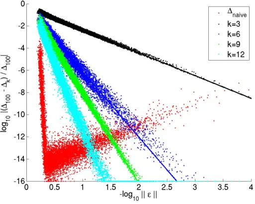
The accuracy of the truncated series expansion can be compared with the naive formula by measuring the JSD between randomly generated probability distributions. Pairs of prob-ability distributions with−4 ≤log₁₀kεk<0, wherekεk =p

(P

nε2n)/N, were randomly generated and the JSD between each pair was calculated by both a direct evaluation of the

(30)

Figure 2.2: Plot comparing the naive and approximate formulae, truncated at different orders for calculating JSD as a function of the normalizedl2-distance (kεk) between pairs

of randomly generated probability distributions. In this figure,∆≡Λ. Best fit slopes are: −2.05(k= 3),−5.89(k= 6),−8.14(k= 9),−11.91(k= 12) and−105.43(comparing naive withk= 100).

exact expression (Λnaive) and the approximate expansion (Λk;k∈ {3,6,9,12}), where Λk= 1 2 X n p_nδnk ; δnk = k X i=1 Biεi_n+1. (2.30)

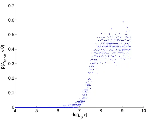
The results shown in Figure 2.2 suggest the series expansion to be a more numerically useful formula when the probability distributions differ by kεk ∼ O(10−0.5_{). Figure 2.3}

further shows that whenkεk ∼ O(10−6_{), a direct evaluation of the exact formula for JSD}

(31)

Figure 2.3: Probability of obtaining (erroneous) negative values, when directly evaluating JSD using its exact expression, is plotted as a function ofkεk. In this figure,∆≡Λ. When implemented inMATLAB, we observe that the naive formula gives negative JSD whenkεk is merely ofO(10−6_).

2.5

Rate of information loss in graph diffusion

We analyze here the rate of loss of predictive information between the relevance variabley and the cluster variablez, during diffusion on a graphG, after the graph nodes have been hard-partitioned intoKclusters.

2.5.1 Well-mixed limit of graph diffusion

For a given partitionQof the graph, defined in equation 2.13, we approximate the mutual informationI[y;z]when diffusion on the graph reaches its well-mixed limit. We introduce

(32)

the lineardependenceη(y, z)such that

p(y, z) =p(y)p(z)(1 +η). (2.31)

This impliesEy[η] = Ez[η] = 0andEy

Ez

η2

= E[η]whereE[·]denotes expectation over the joint distribution andEy[·]andEz[·]denote expectation over the corresponding marginals. Note that the quantityη(·)defined here has no relation to theηdefined in the previous section.

In the well-mixed limit, we have |η| 1. The predictive information (expressed in nats) can then be approximated as:

I[y;z] = E ln p(z, y) p(z)p(y) = Ez[Ey[(1 +η) ln (1 +η)]] ≈ Ez Ey (1 +η)(η−1 2η 2₎ ≈ Ez Ey η+1 2η 2 = 1 2Ez Ey η2 (2.32) = 1 2 X y,z p(y)p(z) p(z, y) p(z)p(y) −1 2 = 1 2 X y,z p(y, z)2 p(y)p(z) −1 ! ≡ι. (2.33)

Here, we defineιas a first-order approximation toI[y;z]in the well-mixed limit of graph diffusion. This quadratic approximation forI[y;z]is known as theχ2_{-approximation.}

Note that the joint and marginal distributions can also be related by the exponential dependenceθ(y, z)defined by

p(y, z) =p(y)p(z)eθ. (2.34) Under this definition, the domain of the dependence is unbounded (i.e. θ ∈ _R) and the mutual information is easily expressed asI[y;z] =E[θ]. We also have

∞ X i=1 Ey θi i! = ∞ X i=1 Ez θi i! = 0. (2.35)

(33)

However, in the well-mixed limit|θ| 1, to first non-trivial order,θ≈ηand the expression forI[y;z]in terms ofθhas the same form as equation 2.32.

We also have η(y, z) = p(z|y) p(z) −1 ≤ 1 p(z) −1 ≤ max z 1 p(z) −1 η(y, z) ≤ max y 1 p(y) −1. ⇒η(y, z)≤min max z 1 p(z) ,max y 1 p(y) −1. (2.36)

Thus, η(y, z)is bounded from below by −1 (by definition) and from above as shown in equation 2.36. However, θ(y, z) is unbounded and negatively divergent for short times. Sinceη is much better behaved thanθ for short times, and for the sake of simplicity, we choose to use the linear dependence instead of the exponential dependence.

2.5.2 Well-mixedK-partitioned graph

As in the IB method, the Markov conditionz−x−yallows us to make several simplifica-tions for the conditional distribusimplifica-tions and associated information theoretic measures. For aK-partitionQof the graph, we have

(34)

p(z) = X x p(z|x)p(x) = X x QzxPx. (2.39)

Graph diffusion being a Markov process, we have P

yGtx0_yG_yxt = G2_xt0_x. Using this and

Bayes ruleGt yxPx=GtxyPy, we have ι = 1 2 X y,z P x,x0QzxGt_yxPxQ_zx0Gt yx0P_x0 (P x00Q_zx00P_x00)Py −1 ! = 1 2 X y,z P x,x0Q_zxQ_zx0P_yGt x0_yGt_yxP_x (P x00Q_zx00P_x00)P_y −1 ! = 1 2 X z P x,x0QzxQzx0( P yGtx0_yGt_yx)Px (P x00Qzx00Px00) −1 ! = 1 2 X z P x,x0QzxQ_zx0G2t x0_xPx (P x00Qzx00Px00) −1 ! . (2.40)

In the hard clustering case,P

xQzxPx=p(z) = [QPQT]zz and we have ι = 1 2 X z [Q(G2tP)QT]zz [QPQT_] zz −1 ! . (2.41)

2.5.3 Well-mixed 2-partitioned graph We can re-writeιas ι = 1 2Ez Ey η2 = 1 2Ey Ez (p(z|y)−p(z))2 p(z)2 . (2.42)

For a bisectionhof the graph,z∈ {+1,−1}and we have

p(z|x) = 1 2(1±hx)≡ 1 2(1 +zhx). (2.43) p(z|y) = 1 p(y) X x p(z, y, x) = 1 p(y) X x p(z|x)p(y|x)p(x) = 1 2 X x (1 +zhx)p(x|y) = 1 2(1 +zhh|yi). (2.44)

(35)

The mutual informationI[y;z]can then be approximated as

ι = 1 2 Ey (hh|yi − hhi)2 1− hhi2 = 1 2 σ2 y(hh|yi) 1− hhi2 . (2.48)

Using Bayes rulep(x|y)p(y) =p(y|x)p(x), we have

Again, graph diffusion being a Markov process,

Ey hh|yi2 = X x,x0 hxhx0p2t(x0|x)p(x) = E2t[hxhx0]. (2.51)

(36)

Time dependence is explicitly denoted here to highlight the fact that diffusion on the graph is till time2t. Substitutinghh|yiin equation 2.48, we get

σ2₍_h_h_|_y_i_{) =} _E y hh|yi2 − hhi2 = E2t[hxhx0]− hhi2. (2.52) ι = 1 2 E2t[hxhx0]− hhi2 1− hhi2 . (2.53) 2.5.4 Fast-mixing graphs

When diffusion on a graph reaches its well-mixed limit in short times, we have G2t ≈

1−2t∆P−1, where1is the identity matrix. Thus, for aK-partition of a graph

Q(G2tP)QT ≈ Q(P−2t∆)QT

= QPQT−2tQ∆QT. (2.54)

For bisections, the short-time approximation ofE2t[hxhx0]can be written as

E2t[hxhx0] = X x,x0 hx0p2t(x0, x)hx = hTG2tPh ≈ hT(1−2t∆P−1)Ph = hTPh−2thT∆h = 1−2thT∆h. (2.55)

Note that this approximation toE2t[hxhx0]makes no assumption about the choice of prior

distributionPon the nodes of the graph. Furthermore, if the discrete-time diffusion oper-ator is used instead,E2t[hxhx0]does not approximate tohT∆hin such a simple manner.

For discrete-time diffusion, the conditional distributionp(y|x)is given as

e Gs yx =p(y|x) = Adiag(d)−1s yx (2.56)

wherediag(d)is the diagonal matrix of node degrees,Ais the adjacency matrix andsis the number of time steps. For anys, substitutingA = diag(d)−∆and expanding the

(37)

binomial gives e G2s = 1−∆diag(d)−12s = 1−2s∆diag(d)−1+ 2s X j=2 (−1)j 2s j ∆diag(d)−1j (2.57)

Thus, forp(x)∝dx, the expression forE2s[hxhx0]becomes

E2s[hxhx0] = 1−2s mh T_∆ h + 2s X j=2 (−1)j m 2s j hT∆ diag(d)−1∆j h (2.58)

From the above equation, we see that even when s = 1, unlike in the continuous-time diffusion case, E2s[hxhx0]does not approximate as simply to the cut andι does not

ap-proximate to the normalized or average cut.

For fast-mixing graphs, the long-time and short-time approximations for I[y;z]and

E2t[hxhx0], respectively, hold simultaneously.

I[y;z] (t)≈ ι(t) ≈1 2−th T_∆ h 1−hhi2 ⇒dI[y;z]/dt≈ dι/dt ∝    A ; p(x)∝1 N ; p(x)∝dx. (2.59)

We have shown analytically that, for fast mixing graphs, the heuristics introduced by Shi and Malik are proportional to the rate of loss of relevance information. The error in-curred in the approximations I[y;z] ≈ ι and E2t[hxhx0] ≈ 1−2thT∆h can be defined

as E₀(t) = E2t[hxhx0]−(1−2thT∆h) E2t[hxhx0] (2.60) E₁(t) = I[y;z] (t)−ι(t) I[y;z] (t) . (2.61)

2.6

Numerical experiments

The validity of the two approximations can be seen in a typical plot of E0(t) and E1(t)

(38)

distributions over the nodes. E1, as seen in figure 2.4, is often found to be non-monotonic

and sometimes exhibits oscillations. This suggests definingE∞, a modified monotonic ‘E1’:

E∞(t)≡max

t0_≥_t E1(t

0_).

(2.62)

E∞(t) is the maximum of E1 over all time greater than or equal to t. We do not need

to define a monotonic form for E0 since this error is always found to be monotonically

increasing in time.

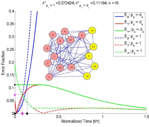
Figure 2.4: E1 and E0 vs normalized diffusion time for two choices of priors over the

graph nodes. E₁ (red) typically tends to have a non-monotonic behavior which motivates defining a monotonicE∞(green). Black –px ∝dx, Magenta –px ∝ 1. H–E∗,n–˜t∗−,u–

˜ t∗₊.

By fast-mixing graphs, we mean graphs which become well-mixed in short times, i.e. graphs for which both the long-time and short-time approximations hold simultaneously

(39)

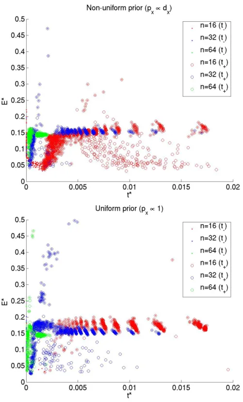
within a certain range of time˜t∗− ≤˜t≤˜t∗+, as illustrated in figure 2.4, where we define E(t) = max(E∞(t),E0(t)) (2.63) E∗ = min t E(t) (2.64) ˜ t∗− = min(arg min ˜ t E(˜t)) (2.65) ˜ t∗₊ = max(arg min ˜ t E(˜t)). (2.66)

E(t) is the larger of the modified long– and short–time errors,E∞andE0, at time t. E∗ is

the minimum ofE(t)over all time. For some graphs, the plot ofE(t)at its minimum might exhibit a plateau instead of a single point, as in figure 2.4 (for prior proportional to degree). ˜

t∗−and˜t∗+denote the left– and right– limits of this plateau. Note that the use ofE∞instead

ofE₁overestimates the value ofE∗_{; the}_E∗_{calculated is an upper bound.}

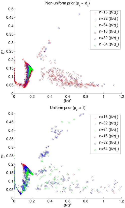
Graphs were drawn randomly from a Stochastic Block Model (SBM) distribution, with block cardinality2, to analyze the distribution ofE∗_,_t_˜∗

− andt˜∗+. As is commonly done in

community detection [Danonet al., 2005], for a graph ofN nodes, the average degree per node is fixed atN/4for graphs drawn from the SBM distribution: two nodes are connected with probabilityp+if they belong to the same block, but with probabilityp−< p+, if they

belong to different blocks. The two probabilities are, thus, constrained by the relation

p+ N 2 −1 +p− N 2 = N 4 (2.67)

leaving only one free parameterp− that tunes the ‘modularity’ of graphs in the

distribu-tion. Starting with a graph drawn from a distribution specified by ap−value and

speci-fying an initial cluster assignment as given by the SBM distribution, we make local moves — adding or deleting an edge in the graph and / or reassigning a node’s cluster label — and search exhaustively over this move-set for local minima ofE∗. Figure 2.5 compares the values ofE∗ and˜t∗−,˜t∗+ for graphs obtained in this systematic search, starting with

a graph drawn from a distribution with p− = 0.02 and N = {16,32,64}. We note that

the scatter plots for graphs of different sizes collapse on one another whenE∗ is plotted against normalized time, confirming the Fiedler value1/τ to be an appropriate character-istic diffusion time-scale [Zivet al., 2005]. A plot ofE∗against actual diffusion time shows that the scatter plots of graphs of different sizes no longer collapse (see figure 2.6).

(40)

Figure 2.5: E∗_vs_˜_t∗_{for graphs of different sizes and different prior distributions over the}

(41)

Figure 2.6: E∗_vs_t∗_{for graphs of different sizes and different prior distributions over the}

(42)

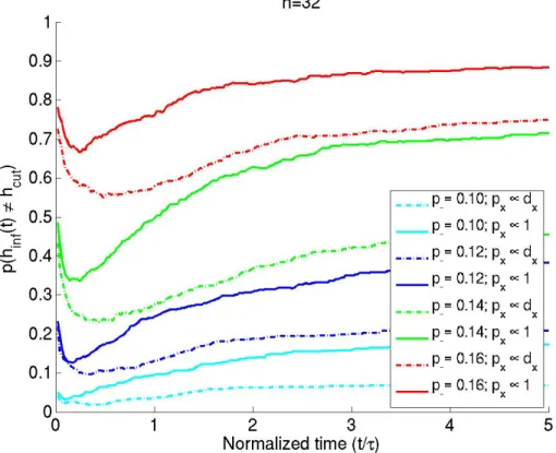
Having shown analytically that, for fast mixing graphs, the regularized mincut is ap-proximately the rate of loss of relevance information, it would be instructive to compare the actual partitions that optimize these goals. Graphs of sizeN = 32 were drawn from the SBM distribution withp− = {0.1,0.12,0.14,0.16}. Starting with an equal-sized

par-tition specified by the model itself, we performed iterative coordinate descent to search (independently) for the partition that minimized the regularized cut (hcut) and one that

minimized the relevance information (hinf(t)); i.e. we reassigned each node’s cluster label

and searched for the reassignment that gave the new lowest value for the cost function be-ing optimized. Plots comparbe-ing the partitionshinf(t)andhcut, learned by optimizing the

two goals (estimated using 500 graphs drawn from each distribution), are shown in figure 2.7.

Figure 2.7: p(hinf(t) 6= hcut) vs normalized diffusion time, estimated using 500 graphs

drawn from a distribution parameterized by a givenp−value, is plotted for different graph

(43)

2.7

Concluding remarks

In this chapter, we have shown that the normalized cut and average cut, introduced by Shi and Malik as useful heuristics to be minimized when partitioning graphs, are well ap-proximated by the rate of loss of predictive information for fast-mixing graphs. Deriving these cut-based cost functions from rate-distortion theory gives them a more principled setting, makes them interpretable, and facilitates generalization to appropriate cut-based cost functions in new problem settings. We have also shown that the inverse Fiedler value is an appropriate normalization for diffusion time, justifying its use in the network infor-mation bottleneck algorithm to capture long-time behaviors on a network.

Absent from this derivation is a discussion of how not to overpartition a graph, i.e. a criterion for selectingK, when employing spectral graph partitioning or the network in-formation bottleneck algorithm. It is hoped that by showing how these heuristics can be derived from a more general problem setting, lessons learned by investigating stability, cross-validation or other approaches may benefit those using min-cut based approaches as well. Furthermore, a derivation of some rigorous bounds on the magnitude of the approx-imation errors, under some conditions, and analysis of algorithms used in rate-distortion theory and min-cut minimization are highly promising avenues for research.

(44)

Chapter 3

Identifying virus hosts from sequence

data

3.1

Context

Emerging pathogens, exemplified by the West Nile outbreak in New York (1999), SARS outbreak in Hong Kong (2003), H1N1 influenza outbreak in Mexico and the US (2009), and the more recent cholera outbreak in Haiti (2010) and E. coli outbreak in Germany (2011) are a critical threat to human society. Rapid and effective public health measures during viral epidemics typically involve identifying and classifying an outbreak from unusual clinical diagnoses, characterizing and restricting viral transmission, and development of appropriate vaccines and treatments. An integral part of this response is the accurate iden-tification and characterization of the virus and understanding what molecular changes in the virus facilitated human infection; a notoriously difficult task in the initial stages of the outbreak when, often, very little reliable, biological information about the virus is known. Complete identification of an organism involves determining the sequence of its genome — a unique blueprint that encodes all the information necessary for the organism to func-tion, within the context of its environment, and reveals details of its evolutionary history. Spurred by rapid advances in high-throughput sequencing technologies, genome sequenc-ing has become one of the most promissequenc-ing and reliable tools to identify and characterize a novel organism. For example, LUJO was identified as a novel, very distinct virus after the

(45)

sequence of its genome was compared to other arenaviruses [Brieseet al., 2009].

This chapter will primarily focus on the goal of predicting the host of a virus from the viral genome. The most common approach to deduce a likely host of a virus from the viral genome is sequence / phylogenetic similarity (i.e., the most likely host of a particular virus is the one that is infected by related viral species). Host inference from phylogenetic trees is consistent with our picture of evolution. Molecular phylogenetic trees constructed using multiple alignment or maximum likelihood methods have been used extensively to determine the original host and evolution of a variety of pathogens. Examples include the swine-origin H1N1 influenza virus [Smithet al., 2009], influenza A virus [Nelson and Holmes, 2007], human immunodeficiency virus [Rambautet al., 2004], andVibrio cholerae

[Chinet al., 2011].

Inference of phylogenies from sparse data, however, is both statistically difficult and methodologically contentious. Techniques based on sequence similarity can also give am-biguous and misleading results when dealing with species very distant to known, anno-tated species. Additionally, armed with a phylogenetic tree, one still requires a principled and accurate assessment of how placement in the tree should be interpreted as association to a host. Moreover, lacking from these techniques is the ability to identify host-specific motifs that can allow us to understand the essential functional changes that enabled the virus to infect a new host. Alternative approaches used in the virus community are typi-cally based on the fact that viruses undergo mutational and evolutionary pressures from the host. For instance, viruses could adapt their codon bias for a more efficient interac-tion with the host translainterac-tional machinery or they could be under pressure of deaminating enzymes (e.g. APOBEC3G or HIV infection). All these factors imprint characteristic signa-tures in the viral genome. Several techniques have been developed to extract these patterns (e.g., nucleotide and dinucleotide compositional biases, and frequency analysis techniques [Touchon and Rocha, 2008]). Although most of these techniques could reveal an underly-ing biological mechanism, they lack sufficient accuracy to provide reliable assessments.

Another promising area of research is metagenomics, in which DNA and RNA sam-ples from different environments are sequenced using shotgun approaches. Metagenomics provides an unbiased understanding of the different species that inhabit a particular niche.

(46)

Examples include the human microbiome and virome, and the Ocean metagenomics col-lection [Williamsonet al., 2008]. It has been estimated that there are more than600bacterial species living in the mouth but that only20%have been characterized. Pathogen character-ization and metagenomic analysis point to an extremely rich diversity of unknown species, where partial genomic sequence is often the only information available. Our main goal here is to develop approaches that can help infer categorical characteristics of an organism from subsequences of its genomic sequence (e.g., host, oncogenicity, and drug-resistance). Using contemporary machine learning techniques, we present an approach to learn complex, yet sparse, tree-structured models built from simple decision rules that predict the hosts of unseen viruses, based on the amino acid sequences of proteins of viruses whose hosts are well characterized. Using sequence and host information of known viruses, we learn a multi-class classifier composed of simple sequence-motif based questions (e.g., does the viral sequence contain the motif ‘DALMWLPD’?) that achieves high prediction accuracies on held-out data. Prediction accuracy of the classifier is measured by the area under the ROC curve, and is compared to a straightforward nearest-neighbor classifier. Importantly (and quite surprisingly), a post–processing study of the highly predictive sequence-motifs selected by the algorithm identifies strongly conserved regions of the viral genome, facilitating biological interpretation.

Our approach is to develop a model that is able to predict the host of a virus given its sequence; those features of the sequence that prove most useful are then assumed to have a special biological significance. Hence, an ideal model is one that is parsimonious and easy to interpret, whilst incorporating combinations of biologically relevant features. In addition, the interpretability of the results is improved if we have a simple learning algorithm which can be straightforwardly verified.

3.2

Mismatch feature space

Formally, for a given virus family, we learn a functiong :S → H, whereS is the space of viral sequences andHis the space of viral hosts. The space of viral sequences S is gen-erated by an alphabetAwhere,|A| = 4(genome sequence) or|A| = 20(primary protein

(47)

sequence). Defining a function on a sequence requires representation of the sequence in some feature space. Below, we specify a representationφ:S → X, where a sequences∈ S is mapped to a vector of counts of subsequencesx ∈ X ⊂_ND

0. Given this representation,

we have the well-posed problem of finding a functionf : X → Hbuilt from a space of simple binary-valued functions.

The collected data consist ofN primary protein sequences, denoteds1. . . sN, of viruses whose host class, denotedh1. . . hN is known. For example, these could be ‘plant’,

‘verte-brate’ and ‘inverte‘verte-brate’. The label for each virus is represented numerically asy ∈ Y = {0,1}L _where_y

l = 1if the index of the host class of the virus is l, and whereL denotes the number of host classes. Note that this representation allows for a virus to have mul-tiple host classes. In the remainder of this thesis, we use notation that treats the indexn over examples (anextensiveindex) as different from an index into a specific vector or ma-trix (intensiveindices), i.e. when referring to a vector associated with thenth _{example, we}

use lowercase boldface variables. For example,ynis a label vector associated with thenth example whileynl is thelth_{element of the label vector for the}_nth_example.

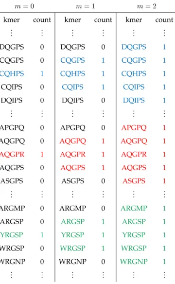
A possible feature space representation of a viral sequence is the vector of counts of exact matches of all possiblek-length subsequences (k-mers). However, due to the high mutation rate of viral genomes [Duffyet al., 2008] [Pybus and Rambaut, 2009], a predictive function learned using this simple representation of counts of exact matches would fail to generalize well to new viruses. Instead, we count not just the presence of an individual k-mer but also the presence of subsequences withinmmismatches from thatk-mer [Leslie

et al., 2004]. Them-neighborhood of ak-merκ, denoted Nm

κ , is the set of allk-mers with a Hamming distance [Hamming, 1950] at mostmfrom it, as shown in Table 3.1. LetδNm κ denote the indicator function of them-neighborhood ofκsuch that

δNm κ (β) =    1 ifβ ∈ Nm κ 0 otherwise. (3.1)

We can then define, for any possiblek-merβ, the mappingφfrom the sequencesonto the number of the elements ofβ’sm-neighborhood insas

φk,m(s, β) = X κ∈s |κ|=k δNm κ (β). (3.2)

(48)

Finally, thedth_{element of the feature vector for a given sequence is then defined}

element-wise as

xd=φk,m(s, βd) (3.3) for every possiblek-merβd∈ Ak, whered= 1. . . DandD=|Ak|.

m= 0 m= 1 m= 2

kmer count kmer count kmer count

..

. ... ... ... ... ...

DQGPS 0 DQGPS 0 DQGPS 1

CQGPS 0 CQGPS 1 CQGPS 1

CQHPS 1 CQHPS 1 CQHPS 1

CQIPS 0 CQIPS 1 CQIPS 1

DQIPS 0 DQIPS 0 DQIPS 1

..

. ... ... ... ... ...

APGPQ 0 APGPQ 0 APGPQ 1

AQGPQ 0 AQGPQ 1 AQGPQ 1

AQGPR 1 AQGPR 1 AQGPR 1

AQGPS 0 AQGPS 1 AQGPS 1

ASGPS 0 ASGPS 0 ASGPS 1

..

. ... ... ... ... ...

ARGMP 0 ARGMP 0 ARGMP 1

ARGSP 0 ARGSP 1 ARGSP 1

YRGSP 1 YRGSP 1 YRGSP 1

WRGSP 0 WRGSP 1 WRGSP 1

WRGNP 0 WRGNP 0 WRGNP 1

..

. ... ... ... ... ...

Table 3.1: The mismatch feature space representation of a segment of a protein sequence ...AQGPRIYDDTCQHPSWWMNFEYRGSP...

Note that whenm= 0,φk,0exactly captures the simple count representation described

earlier. This biologically realistic relaxation allows us to learn discriminative functions that better capture rapidly mutating, yet functionally conserved, regions in the viral genome,

(49)

facilitating generalization to new viruses.

3.3

Alternating decision trees

Given this representation of the data, we aim to learn a discriminative function that maps featuresxonto host class labelsy, given some training data{(x1,y1), . . . ,(xN,yN)}. We want the discriminative function to output a measure of “confidence” [Schapire and Singer, 1999] in addition to a predicted host class label. To this end, we learn on a class of func-tionsf :X →_RL_{, where the indices of positive elements of}_f₍_x₎_{can be interpreted as the} predicted labels to be assigned toxand the magnitudes of these elements to be the confi-dence in the predictions. We will use square brackets to denote the selection of a specific element in the vector output of the discriminative function, i.e.,[f(x)]lis thelth_{element of}

the output of the functionf.

A simple class of such real-valued discriminative functions can be constructed from the linear combination of simple binary-valued functionsψ:X → {0,1}. The functionsψ can, in general, be a combination of single-feature decision rules or their negations:

f(x) = P X p=1 apψp(x) (3.4) ψp(x) = Y d∈Sp I(xd≥θd) (3.5)

whereap ∈RL,P is the number of binary-valued functions,I(·)is 1 if its argument is true,

and zero otherwise,θ∈ {0,1, . . . ,Θ}, whereΘ = maxd,nxnd, andSp is a subset of feature indices. This formulation allows functions to be constructed using combinations of simple rules. For example, we could define a functionψas the following

ψ(x) =I(x5 ≥2)× ¬I(x11≥1)×I(x1 ≥4) (3.6)

where¬_I(·) = 1−_I(·).

Alternatively, we can view each functionψpto be parameterized by a vector of thresh-oldsθp ∈ {0,1, . . . ,Θ}D, whereθpd = 0indicatesψpis not a function of thedthfeaturexd. In addition, we can decompose the weights [Busa-Fekete and Kegl, 2009]ap = αpvp into

(50)

a vote vectorv∈ {+1,−1}L_{and a scalar weight}_α _∈

R+. The discriminative model, then,

can be written as f(x) = P X p=1 αpvpψθp(x), (3.7) ψθp(x) = Y d I(xd≥θpd). (3.8) Root 0.3 [TFLKDELR] ≥ 1 [AKNELSID] ≥ 2 1.5 [AAALASTM] ≥ 1 0.0 0.3 0.4 1.2 0.5

True False True False

True False True 0 2 1 3

˜

ψ

θ3

ψ

θ

3

Figure 3.1: An example of an ADT where rectangles are decision nodes, circles are output nodes and, in each decision node,[β] =φk,m(s, β)is the feature associated with thek-mer β in sequences. The output nodes connected to each decision node are associated with a pair of binary-valued functions(ψ,ψ). The binary-valued function corresponding to thee

highlighted path is given asψe_θ₃(x) = I([AKNELSID]≥ 2)× ¬I([AAALASTM]≥ 1)and

the associatedαe3 = 0.3. Not shown in the figure is the vote vectorvassociated with each

output node.

Every function in this class of models can be concisely represented as an alternating de-cision tree (ADT) [Freund and Mason, 1999]. Similar to ordinary dede-cision trees, ADTs have

(51)

two kinds of nodes: decision nodes and output nodes. Every decision node is associated with a