Interactive Visualization for
Network and Port Scan Detection
Chris Muelder1, Kwan-Liu Ma1, and Tony Bartoletti2 1 University of California, Davis
2 Lawrence Livermore National Laboratory
Abstract. Many times, network intrusion attempts begin with either a network scan, where a connection is attempted to every possible des-tination in a network, or a port scan, where a connection is attempted to each port on a given destination. Being able to detect such scans can help identify a more dangerous threat to a network. Several techniques exist to automatically detect scans, but these are mostly dependant on some threshold that an attacker could possibly avoid crossing. This paper presents a means to use visualization to detect scans interactively.
Key words:Network security, information visualization, intrusion detection, user interfaces, port scans, network scans
1
Introduction
Network scans and port scans are often used by analysts to search their networks for possible security hazards in order to fix them. Unfortunately, these same hazards are exactly what an attacker is also interested in finding so that they can be exploited. Therefore, scanning the computers on a target network or the ports of a target computer are very common first steps in a network intrusion attempt. In fact, any network exposed to the Internet is likely to be regularly scanned and attacked by both automated and manual means [13]. Also, many Internet worms exhibit scan-like behavior, and so for the purposes of detection can be treated similarly [16]. Thus, it is in the best interests of network analysts to be able to detect such scans in order to learn where an attack might be coming from or to enable countermeasures such as a honeypot system.
Also, it is possible to take an attacker’s attempt to gain information about a network through a scan and use it to gain information about the attacker, using methods such as in [14]. That is, a scan can be analyzed in order to identify features of an attacker, such as the attacker’s operating system, the scanning tool being used, or the attacker’s particular hardware. Timing information can even be used to analyze routing delays which can reveal the attacker’s actual location in cases of IP address spoofing. Thus, it is also beneficial to detect scans for counterintelligence purposes.
Previous research has been done in finding ways to automatically detect network and port scans. These methods usually involve distinguishing between
an attacker and a normal user by checking to see if the traffic meets some criteria. However, it is usually possible for an attacker to avoid detection by avoiding meeting the criteria in question. The simplest kind of detection system is to designate a tripwire port or IP address, such that if there is any traffic to that port or IP address, the traffic is designated as a port or network scan respectively. However, this method is essentially just security through obscurity. If an attacker can determine what port or system is being used as a tripwire, it is a relatively simple task to just avoid connecting to that port or system. One of the most common scan detection methods, however, is based on timing thresholds [6]. If traffic from a particular source meets some threshold of connections per unit time to different ports or systems then it is classified as a scan, otherwise it is classified as normal traffic. The difficulty with this method is that if the threshold is too low, then normal traffic can be determined to be a scan, and if the threshold is too high, then scans could be classified as normal traffic. Therefore, if an attacker runs a scan slowly enough to be classified as normal traffic, then it would go undetected entirely.
Visualization provides an alternate approach to solving this problem. Many attempts have been made to ease the detection of interesting information in the logs, using both traditional information visualization mechanisms like parallel coordinates, self-organizing maps, and multi-dimensional scaling, and novel vi-sualization mechanisms designed specifically for this task [4, 3]. Instead of work-ing with the low level timwork-ing information for every packet, however, one can summarize the data and display it for the user to look for patterns. Because it requires human interaction, this is a somewhat more time consuming method and would not be very useful when a quick response time is necessary. However, it provides a high level view of the data, from which patterns such as network or port scans should be easily visible. Visualization also provides a means to detect new and interesting patterns in the information that could be missed by auto-mated rules. From these patterns, new rules can be defined in order to improve the automated methods. This allows an analyst to iteratively refine the rule set, and with each cycle the detection improves.
We have developed effective visualization representations and interaction techniques within a unified system design to address the challenges presented by the complexity and dimension of the traffic information that must be rou-tinely examined. In our study, the (sanitized) traffic data are provided by the Computer Incident Advisory Capability group at the Lawrence Livermore Na-tional Laboratory (LLNL).
2
Related work
This overall method of creating an image of network traffic is not wholly new. SeeNet [1] uses an abstract representation of network destinations and displays a colored grid. Each point on the grid represents the level of traffic between the entity corresponding to the point’sxvalue and the entity corresponding to the point’syvalue. NVisionIP [8] uses network flow traffic and axes that correspond
to IP addresses; each point on the grid represents the interaction between the corresponding network hosts. The points can represent changes in activity in addition to raw activity. In [17], a quadtree coding of IP addresses is used to form a grid; Border Gateway Protocol (BGP) data is visualized as colored quadtree cells and connections between points on the quadtree. The Spinning Cube of Potential Doom [9] is a visualization system that uses two IP address axes and a port number axis to display network activity in a colorful, 3-dimensional cube. The combination makes attacks like port scans very clear; attacks that vary over the IP address space and port number produce interesting visuals (one method of attack, for instance, produces a “barber pole” figure). In [14], scans of class B networks are visualized by using the third and fourth octets of the destination IP addresses as the xand y axes in a grid, and coloring these points based on metrics derived from connection times.
PortVis [11] is a system designed to take very coarsely detailed data—basic, summarized information of the activity on each TCP port during each given time period—and uses visualization to help uncover interesting security events. Similar to the other related works, the primary methods of visualization used by PortVis are to display network traffic by choosing axes that correspond to important features of the data (such as time and port number), creating a grid based on these axes, and then filling each cell of the grid with a color that represents the network activity there. However, all the other related works work with the low level data itself, so they can not scale as large as easily as a system like PortVis that works with summarized information.
This paper presents the design of a port-based visualization system and a set of case studies to demonstrate how the visualization directed approach im-plemented effectively helps identify and understand network scans. Our designs were made according to the lessons we learned from building and using PortVis [11]. This new system offers analysts a suite of carefully integrated capabilities with an interactive interface to interrogate port data at different levels of details. This paper also serves to suggest some general guidelines to those who intend to incorporate visualization into their IDS.
3
A Port Based Visualization System
We have developed a portable system, written in C++ with OpenGL and a GLUT based widget toolkit, that takes general, summarized network data and presents multiple, meaningful perspectives of the data. The resulting visual-ization often leads to useful insights concerning network activities. The system design was tailored to effective detection and better understanding of a variety of port and network scans. However, the system is also capable of detecting other large-scale and small-scale network security events while requiring a minimal amount of data and remaining interactive and intuitive to use.
It is port based, so it should be able to permit analysts to discover the presence of any network security event that causes significant changes in the activity on ports. Since it uses very high-level data, it is a very high-level tool,
and is useful mostly for uncovering high-level security events. Security events that consist of small details—an intrusion that includes only a few connections, for instance—are unlikely to be caught using these methods.
Since information about the network’s size, structure, and other important attributes may be sensitive, it is expedient to look at visualizations that permit network security events to be detected without the use of those attributes. The system was designed to use a very minimal set of aggregate attributes that reveals a minimal amount of information about the network. Since the data consists of only counts of activities (rather than records of the activities themselves), analysis can only go so far. It can identify scans and other suspicious traffic patterns, but it cannot see the traffic that caused the patterns. This is still useful, however; analysts using it can send the suspicious traffic signatures to analysts that have access to the full set of network traffic logs. Also, sometimes the original logs contain information that can not be distributed due to sensitivity concerns or the potential for violation privacy laws. But even if the original traffic logs are sensitive, and can not be disseminated, the summarized data is likely not sensitive and can be distributed and analyzed by third parties.
In addition to mitigating security concerns, using aggregate data results in an immense reduction in storage and transmission requirements. Storing and transmitting detailed data about network activity can be challenging or even impossible for non-trivial periods of time, but if the data is simply aggregated and only the aggregate values are used, these values can be stored and trans-mitted much more efficiently and cheaply, resulting in higher interactivity and explorability of the system.
3.1 Methodology
When dealing with large datasets, often times there is too much data to fit into one view. So visualization methods often employ multiple semantic levels in or-der to be able to present both high-level patterns and low-level details. Then, the user can drill down from higher levels to lower levels to gain insight about interesting patterns in the higher levels. Conversely, the user can gain insights from interesting patterns found in the lower level detailed views that should be confirmed with higher level views. Thus, each level provides contextual informa-tion about the other levels. So it is beneficial to present them all simultaneously to the users, so they can switch between semantic levels without losing context. Also, this improves the speed at which the user can switch between the semantic levels, because the only work involved is a glance to a different region of the screen.
Our system uses three basic semantic levels: a high-level overview that shows the entire dataset at low resolution, a mid-level view that shows all ports at one point in time, and a low-level detailed view that shows an individual port over all metrics for the whole time range of the dataset. In general, the methodology of visualization used in this system starts at a high semantic level then drills down into regions of interest. For example, an analyst might start with a high-level timeline view of the dataset and notice a pattern that could be indicative of a
scan at a particular time. Then the analyst would likely proceed to view just this time with more detail in the mid-level view that shows all ports. Finally, one particular port or range of ports could stand out and warrant investigation with the low-level view. In order to make this drilling down process more intuitive, the views have been laid out from left to right, such that each view represents a progressively lower semantic level.
At each level, several visualizations are used, because they are useful at de-tecting different kinds of patterns. For instance, it is possible that there is an interesting pattern in the high-level view does not show up in the current mid-level view. Conversely, one might find a pattern in a lower mid-level that is not apparent in a current higher level view. So, it is beneficial to allow the user to switch particular views to ones that a pattern of interest does show up in. But while there are one or more different visualizations employed per level, usually only one is used at a time per level. This insures that the contexts between se-mantic levels are preserved, while not overloading the user with too many views at once.
3.2 System Components and Interface
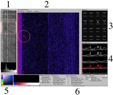
Fig. 1. The entire application. The layout of components from left to right is made according to a drill-down process of visual interrogation.
There are three main semantic levels: the timeline, the time instant, and the port. Each has its own visualizations. As can be seen in Figure 1, all the seman-tic levels are present simultaneously, so it is easy to correlate data and mentally
shift between visualizations. Visualization generally begins at the timeline (1), followed by a time instant (grid or scatterplot) visualization (2). The grid vi-sualization contains a circle, which helps users locate the magnification square in its center. Magnifications from the square within the main visualization are shown in (3); a port may be selected from (3) to get the port activity display in (4). Several parameters (5) control the appearance of the main display and port displays. The panel of options in (6) permits the selection of a data source to display, and offers a color-picker for selecting new colors for gradients.
The timeline visualization Thetimeline is a visualization of the entire time range available. It shows a compressed 2D view, which has several elements. The vertical axis corresponds totime. Each row of the visualization represents one unit of time. The top row is the earliest time unit for which there is data; the bottom row is the latest time unit for which there is data. The horizontal axis corresponds to port range. Each row consists of 32 columns, each of which represents 65,536÷32 = 2,048 ports. The leftmost column corresponds to the
first 2,048 ports, the next column to the right corresponds to the next 2,048 ports, and so forth. The color of the column is determined by the level of activity on the ports during the time unit. The selector (the red box) corresponds to the currently selected time. This is the time unit that is displayed on the grid visualization panel.
The histogram near the bottom corresponds to the relative frequencies of each activity level over the entire range of time. “Activity level” here means “number of sessions.” Therefore, if a very large number of ports have the same activity level, there will be a spike in the histogram at that activity level. The goal of the histogram is to provide information on activity levels so that they can be usefully mapped to colors. Note that all of the analyses of activity levels in the timeline window are done on a log scale; this is necessary because there are generally several ports with very high levels of activity (for instance, port 80), and these would irreparably skew a normal scale.
Finally, the gradient editor below the histogram corresponds tothe mapping from activity level to color. The gradient editor can be used to explore spikes, gaps, or other interesting features of the activity level space revealed in the his-togram by mapping each activity level to a smoothly interpolated color. Any number of arbitrarily colored control points can be added to the gradient; col-ors are linearly interpolated between control points. In general, operatcol-ors are interested in seeing indications of port activity above certain levels [19], and the gradient editor can act as a filter to achieve this end.
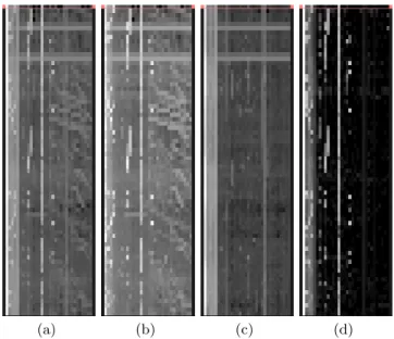
Figure 2 shows some examples of timelines based on different metrics. Dif-ferent metrics can reveal difDif-ferent patterns in the data. The basic session count metric (a) gives a basic overall feel for the amount of activity on a network, however, when searching for something particular like scans, there are better alternative views such as the ratio of destination addresses to source addresses (b). In this view the scan patterns that can be seen in (a) are more clearly defined. Other views such as the difference between the session count and the
unique source/destination pairs count (c) can be useful for detecting anomalies such as covert communications, but are nearly useless for detecting scans be-cause it essentially filters out scan activity, leaving only repeated connections. Another interesting view is the difference between the number of sessions and the number of source addresses (d). This essentially filters out the port scans, leaving network scans and maintained connections.
(a) (b) (c) (d)
Fig. 2.Timelines with different metrics.
The grid visualization The grid visualization depicts the activity during a given time unit. It consists of a dot on a 256×256 grid for each of the 65,536
ports. The port number can be thought of as a two-byte number. Therefore, thex (horizontal) axis represents thehigh byteof the port number, and they(vertical) axis represents the low byte of the port number. So each point corresponds to a particular port, and the color of each point is determined by the value of the current metric at the corresponding port. Points for which there exists no data (probably because there was no activity at all on the port) are always black. A small, square selector (1) corresponds tothe ports currently being magnified. The selector is 4×4 grid units in size and can be dragged around with the mouse to
magnify any group of ports the user desires. A large circle (2) serves tohelp users locate the selector. The selector is relatively small, and can easily get lost in the field of ports, especially when there is a lot of background noise. A magnification area (3) serves to provide detailed information about the magnified ports. Each port’s exact number is displayed, along with an enlarged visualization of its color point—to help users correlate it to the main visualization—and its exact data
value. A histogram (not shown) corresponds to the the relative frequencies of each data value. Like the histogram in the timeline, it serves to identify trends and/or patterns in the data. A gradient editor (not shown) corresponds to the the mapping from data values to colors. Like the gradient editor in the timeline, it helps users explore gaps, spikes, and other interesting features that may be noticeable in the histogram.
Fig. 3.The grid visualization.Session counts are shown with a blue to white gradient. A small region around port 46011 has been zoomed into.
The scatterplot Thescatterplotwas added to help analysts compare the differ-ent metrics. Scatterplots have been applied to security visualizations in previous work [5, 10]. The scatterplot is an alternative to the grid visualization since it is at the same semantic level. The primary difference is that instead of laying the ports out by their numeric value, they are laid out according to the values of two metrics for that port. Some features that are difficult to see in the grid view become quite obvious in a scatterplot and some patterns that are obvious in the grid view are nearly invisible in the scatterplot. For example, to find a network scan in the grid based requires hunting for a small area with a different color, which can be difficult. But in a scatterplot, one can just look at the ports that fall in a certain region and deduce that they are likely network scans. However, while a port scan is quite visible in the grid visualization, in a scatterplot all the ports involved will occlude each other, making it impossible to see a pattern.
The axes of the scatterplot correspond to two different metrics and each point in the scatterplot is a particular port. The color is determined just like the
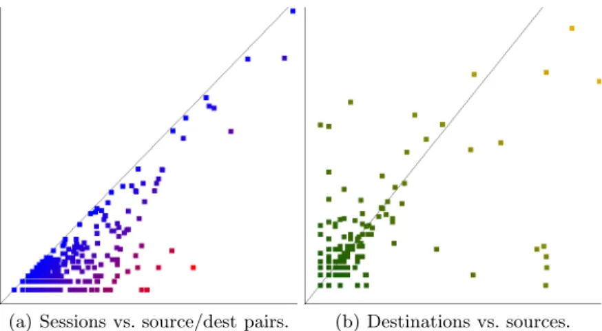
grid visualization, but the position is determined by the values of the metrics that the axes correspond to. The same histogram and gradient editor that are used by the grid visualization are used to control the scatterplot. Figure 4 shows some examples of this method. Figure 4(a) shows the total number of sessions on the xaxis versus the number of different unique pairs of sources and desti-nations on the y axis. This is useful when looking for maintained connections such as covert communications, because it essentially isolates cases where a few computers were making a lot of connections. Figure 4(b) shows the number of destination addresses versus the number of source addresses. Network scans have a low source count and a high destination count, so they fall into the lower right region of this scatterplot. The upper left region however, corresponds to ports that had high source counts and low destination counts, such as would occur in a distributed denial of service attack.
(a) Sessions vs. source/dest pairs. (b) Destinations vs. sources.
Fig. 4. The scatterplot visualization.Per port values are positioned based on their values in two different metrics instead of by the port number.
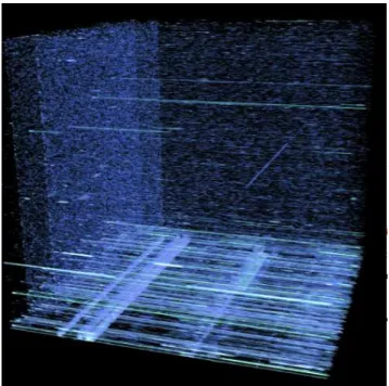
The volume visualization The representation of the timeline works very well for analyzing up to several hundred time units of data at once, but as the num-ber of time units reaches the numnum-ber of rows of pixels available, detail is lost. Alternative representations of time exist; for instance, [12] describes a method for compacting a timeline of arbitrary length into a visualization of constant size. The other option is to add one more dimension to the visualization so more information may be presented. Each row in the previous timeline visualization becomes the 2D plane that the grid visualization would generate, displaying a selected attribute for every port. With time as the third dimension, a volume is formed. In order to view this volume interactively, a hardware accelerated volume renderer was used. Figure 5 shows a volume rendered image of such a
representation that gives essentially an expanded view of the same information that the other views provide. The axes of the volume in this particular image are time going from left to right, high byte going from bottom to top, and low byte going from front to back.
Fig. 5. This 3D volume visualization provides an overview of time-varying port at-tributes using volume rendering.
The volume rendering has the advantage of not needing another visualization at the time instant semantic level, because it displays all of the data at once. However, the dataset is not very conducive to volume rendering. The features of interest are quite often only one or two voxels across, so they could easily be missed. Also, occlusion and noise can make it very difficult to see interesting patterns. But it still provides a nice way to see the whole dataset without having to go back and forth between several panels.
The port visualization The timeline visualization can identify a particular block of ports at particular time that warrant further investigation. The main visualization can often—as in Figure 3—identify specific ports(s) to be investi-gated. But, given that information, one question remains:is the identified activity on the port anomalous? This question is addressed by the remaining visualiza-tion technique, which is a view of all the data available that concerns a particular port.
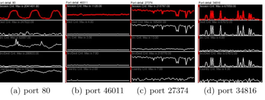
(a) port 80 (b) port 46011 (c) port 27374 (d) port 34816
Fig. 6. The port visualization.Plots of metrics versus time for individual ports. In each example, the session count (the first metric) is highlighted. The other 4 metrics shown are destination address count, source address count, unique source and destina-tion pair count, and source country count. These ports show a few distinct patterns of activity.
Figure 6 displays the components of the port visualization. Each of the par-allel graphs correspond to a particular data metric. The vertical axes correspond to thedata values; the greater the value, the more height. The horizontal axis corresponds to time. The time currently being analyzed is indicated by a red bar. And finally, the attribute that is currently being analyzed with the main visualization is highlighted in red.
Examples of some ports are given in Figure 6. The usage of Port 80 is very periodic; it goes up during the day, and, predictably, down during the night. Port 46011 has a fairly constant level of activity, with a few spikes. Port 27374 is more erratic, though, interestingly, its usage drops noticeably as time goes on. Port 34816 has one of the most suspicious usage graphs; it is only used a few times, but it is used fairly heavily during those times.
Comparing and contrasting It is often the case that a network analyst is not interested so much in what occurred during a particular time unit but rather what changed across a range of time units. [8] Therefore, a feature was imple-mented that allows analysts to select any arbitrary set of time units and see on the grid visualization not a depiction of theactualvalues at each port but rather a depiction of thevariance of the values at each port. Suppose, for instance, that the analyst selected 4 units of times, during which the port had 1,434 sessions, 1,935 sessions, 1,047 sessions, and 1,569 sessions, respectively. The system would then assign that port a value equal to theσ2 of this set of values.
However, a large absolute variance on port 80 is a lot less interesting then the same variance on some random high numbered port such as port 12345. This is because the average value of a metric on port 80 would be expected to be much larger then on port 12345. So in order to prevent values from common ports such as port 80 from overwhelming the rest of the data, the capability was added to view relative variance. This is calculated by dividing the variance calculated for
each port by the average value for that port. Thus, while a variance of 1,000 would be the same on port 80 or port 12345, the relative variance for port 80 would likely be very small, while the relative variance on port 12345 would probably be quite large. So the capability to calculate the relative variance over a range of time was added. Using this statistical method can sometimes bring out interesting patterns that were previously unseen. In figure 7(a), the variance over the whole dataset was calculated. While several interesting ports show up, any pattern that shows up is quite faded, if visible at all. However, when the relative variance is calculated instead, as in figure 7(b), the patterns show up distinctly. In particular, there is a suspicious line down the middle of the image that is completely invisible in the left image.
(a) Variance (b) Relative variance Fig. 7. Variance calculations.
During the course of a day, the amount of traffic on a network will naturally vary substantially. This effect can be seen quite clearly in the oscillating pattern on port 80 shown in figure 6 This can skew some of the results, as natural traffic will have variance but attacks can have relatively low variance. However, one would expect that as traffic levels rise and fall, the percentage of traffic that occurs on a particular port will be relatively constant. That is, if approximately half the traffic is on port 80 at midday, approximately half the traffic should be on port 80 at midnight as well. Therefore, in order to counter the natural variance, one can normalize the data into percentages of the total amount at a particular time. So the option was added to allow to normalize the data before calculation of variance.
4
Case studies
The data sets used in our study were collected by a number of network traffic analyzers installed at the Internet gateway of selected Department of Energy sites. These traffic analyzers summarize large amounts of Internet Protocol (IP) traffic that flows to/from the Internet. As a result of the summarization, the data
is reduced to a set of counts of entities. For instance, instead of a list of each TCP session, there is a field that specifies how many TCP sessions are present; instead of a list of source IP addresses, a field specifies how many different source IP addresses were present. While the raw data is unclassified, it is handled as Official Use Only (OUO), and is therefore restricted, but the summarized data is not, and so it is not restricted.
The full list of fields present appears in Table 1. The first three fields are used for filtering and positioning the data; the last five fields are considered to be attribute values. The fields in combination tell a much more useful story than any individual field. For instance, suppose that a port has a relatively high session count. What does this represent? If many sources and one destination are involved, it could be a distributed denial of service attack, in which many systems attack one system, often targeting a service on a specific port. If many destinations and one source are involved, it could be a network scan or worm attack, in which a single attacker or group of attackers probes a number of des-tination machines on the same port, looking for a vulnerable service. If only a single source and destination are involved, it could be a TTL walking attack, in which an attacker probes a machine 50–100 times in an attempt to deter-mine the network topology through TTL variations. Therefore, information on the uniqueness of source addresses, destination addresses, and pairs of the two is very useful to analysts. In particular, the number of unique pairs provides a redundancy-free measure of the extent to which a port seems broadly inter-esting to the community of adversaries—a measure that is very difficult for an individual attacker to skew.
Since certain patterns are more visible by looking at pairs of these attributes, the capability was added to calculate functional combinations of these five base metrics given in the raw data. Currently, the only functions that work are the four basic math operations (+,−,∗, and/), but these still can still reveal many
interesting features. For example, network scans tend to stand out when one looks at the ratio of destinations to sources.
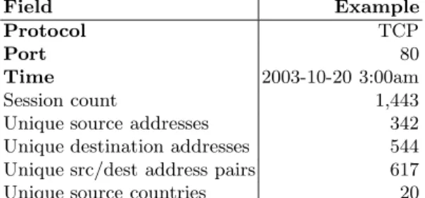
Table 1. The fields available, and an example of each.Each tuple representsthe activity on a given port during a given time period, through the given protocol. The first three fields (Protocol, Port, and Time) form a unique, composite key. The example row here is fictitious. Field Example Protocol TCP Port 80 Time 2003-10-20 3:00am Session count 1,443
Unique source addresses 342
Unique destination addresses 544 Unique src/dest address pairs 617
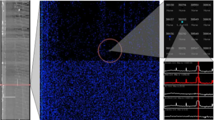
Figure 8 demonstrates how the drill down methodology works for finding network scans by applying it to a 24 hour long dataset at 10 minute resolution. Since we are looking for network scans, the metric being shown has been selected to be the ratio of destinations to sources. Then, starting at the timeline on the left, a spike is found on a high port that crosses several hours. One of these hours is then selected for viewing in the grid based visualization. In it, there is exactly one port with unusually large values in the range of ports that correspond to the column in the timeline that has the spike. So the range around this port is zoomed into which generates the third image (the one in the upper right). Finally, the particular port of interest, which happens to be port 38293, is selected to be shown in the port view. As can be seen in this view, there was an abnormally large number of destinations being connected to by such a small number of sources, which means that this is probably a network scan. Also of note is that the duration of the scan on this port corresponds with the duration of the spike seen on the timeline. A quick check through the hourly views during this duration also confirms that there were no other ports contributing substantially to the spike in the histogram, meaning that the spike is caused by this port alone.
Fig. 8. Methodology example.Systematically discovering a network scan.
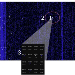
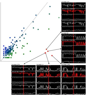
Network scans can be even easier to detect with the scatterplot then with the grid based display. Rather than requiring the user to hunt through a range of ports looking for the one that is a different color, the scatterplot can be used to isolate ports with network scans away from the rest of the ports. For example, in figure 9, the scatterplot has been used to identify several possible network scans. The scatterplot was generated with the source count metric on the y axis, and the destination count metric on thexaxis, because network scans are distinctive in that they have high destination counts and low source counts. Therefore, they should fall into the lower right corner of the plot, and during the hour of interest shown in the figure, there were 5 such ports that stood out strongly. As can be seen in the figure, they all actually do have high destination counts and low
source counts, meaning that there was likely a network scan running on each port during that hour.
Fig. 9. A scatterplot showing destinations versus sources. The ports that are in the lower right are probable network scans.
While network scans focus on single ports or small groups of ports, port scans usually cover a large range of ports, possibly up to all 65536 ports. In Figure 10, two port scans are shown. The scan on theleft is a “randomized” scan; over the period of a few hours, the scanner hit ports at random, eventually trying all of them. Network activity was fairly normal at first, but random port hits increased gradually, and during the final hour, nearly every port was hit. The scan on the right is a linear scan that was also run over a few hours. The scanning formed every-other-port stripes that covered most of the upper port range (the missed ports were covered in a subsequent scan, which is not shown here). Note that both the randomized (top) and linear (bottom) scans stand out on the timeline, making them easy to tag for this kind of detailed analysis.
Figure 11 demonstrates another way the system can be used for the detection of port scans. The dataset in this example covers three and a half days at one hour resolution. The first of the series of images shows the initial timeline view. In it, several diagonal lines can be faintly seen running through the timeline. In order to accentuate these lines, the gradient editor was used to show them with
Fig. 10.Two port scans: A rapid randomized scan and a slow sequential scan
high contrast in the second image. The third image highlights five of the possible port scans discovered in this way. They can also be seen as planes in the volume rendered view, as is shown in the fourth image. Note that these scans take place over several hours each, so it is possible that they are slow enough that they would not be picked up by a simple statistical detection program.
Fig. 11. This timeline visualization provides an overview of the collected data in a highly compact fashion.
Figure 12 shows the variance analysis system in action. When the timeline for this dataset was viewed with the ratio of destinations to sources metric, a region showed a suspicious block of heavy activity on the lower half of the port
space over an entire day. When any of these times are viewed directly with the grid visualization, they just show random noise over the port range. However, calculating the variance over this time range reveals an interesting striation pattern in the range of ports being scanned, as can be seen in the figure. This pattern could be indicative of the order that the ports were scanned or the tool that was used. Or it is possible that it is just an artifact from the reduction to hourly counts, in which case higher resolution data would be required. In either case, explaining the pattern definitively would require access to more detailed data.
Fig. 12. The variance visualization.Looking at the variance reveals probable port scan activity.
5
Conclusion
Among other anomalous features, port scans and network scans can often be seen quite readily with these methods. Even with the limitations on the data, many interesting security features can be detected and identified. Sometimes the cause of the interesting features can not be determined without using some other methods, but knowing where the other methods should be applied is useful. However, the techniques used are not bulletproof. Network scans that occur on ports that are commonly used could easily go undetected, simply because the normal usage overwhelms it. Port scans that are performed slowly enough with a random order would also be very difficult to detect, because they would be ignored as being noise. However, this problem could be overcome by refining and
reducing the data. That is, once scans are detected with a given time interval, filter them out and increase the time interval. Then slower scans would show up without being overwhelmed by the more rapid scans. Overall, the tool manages to give a high level view into the status of a network without sacrificing the confidentiality of a network’s infrastructure, and provides a rapid way to detect both network and port scans.
6
Future work
There is a limit to what can be done with summarized data; a large amount of interesting work lies in the integration of more detailed data about network activity. If IP addresses and other information about each session were incor-porated, the existing visualizations could be made much more richly detailed, and new visualizations could be created that could lead to insights that cannot be found in summarized data. For example, being able to adjust the resolution of the summarization dynamically could make the timeline a good zoomable interface. In fact, it would be a good idea to add access to the full data as a modular plug-in, so that in house analysts can access the full data, while the basic summarized visualizations are usable even by third parties.
These visualization techniques were all developed based on summarizing the data by port. It is also possible to summarize the data based on source addresses or destination addresses, and apply the same visualization methods. For source address summarization, the data values could be session count, destination ad-dress count, port count, and unique destination adad-dress and port pairs. And for destination address summaries, The values could be session count, source address count, port count, and unique source address and destination port pairs. These different metrics would be able reduce the sensitive nature of the original data just like the port summarization, and would provide another view of the data. The combination of these various summarized datasets could allow the user to gain a more insightful view of the data then any one dataset alone.
Currently, human pattern detection is relied upon to find patterns in the data and groups of related ports. However, machine learning could be poten-tially applied to find patterns and anomalies, augmenting human abilities. Since the techniques being used do not label the data, clustering algorithms are likely to be of use, since these have proven to be useful in discovering security events in unlabeled data. [15] For instance, a self-organizing map [7] or multi-dimensional scaling technique [18] could be used to organize the ports according to their nearness in data space (similar to [4]), hopefully isolating the ports with un-usual usage. Another machine learning approach to finding interesting outliers is discussed in [2].
Once these scans are detected, there is still the question of what to do with them. Given the limited dataset used in this project, there is not much more that can be done. However, one can take information gained from looking at this summarized data and isolate a scan in the original data. Then, analysis can be done on more precise information such as the timing of packets to different
destination addresses or ports. Some visualization and statistical techniques for performing such an analysis have been developed by Bryan Parno and Tony Bartoletti [14], and work is currently being done to extend these methods.
There are several other statistical calculations that could be used to view change over ranges of time instead of the variance based methods currently used. The standard deviation and the coefficient of variation would make good alternatives for variance and relative variance respectively, because they serve essentially the same purpose. They also would have the advantage of preserv-ing units, at the cost of bepreserv-ing slightly more computationally expensive. The covariance or correlation between pairs of metrics could also make an interesting measurement.
It would also be useful for the system to have the capability to save and restore visualization states, so that interesting views could be easily recalled. Very useful views could evolve into a kind of “at-a-glance” network visualization system. The system’s responsiveness could also be improved; currently, it reads data from the raw text files and computes its statistics. It would save the user time if some of the calculations were pre-processed and stored so that data loaded more quickly upon startup.
7
Acknowledgements
We would like to thank the DOE Computer Incident Advisory Capability (CIAC) operation at LLNL for providing the data upon which this exploration was based. We would also like to thank Andrew Brown for his ready assistance in extracting and providing the statistical data
References
1. Richard A. Becker, Stephen G. Eick, and Allan R. Wilks. Visualizing network data. IEEE Transactions on Visualization and Computer Graphics, 1(1):16–28, 1995.
2. P. Dokas, L. Ertoz, V. Kumar, A. Lazarevic, J. Srivastava, and P. Tan. Data mining for network intrusion detection. InProc. NSF Workshop on Next Generation Data Mining, 2002.
3. Robert F. Erbacher. Visual traffic monitoring and evaluation. InProceedings of the Conference on Internet Performance and Control of Network Systems II, pages 153–160, 2001.
4. L. Girardin and D. Brodbeck. A visual approach for monitoring logs. InProceedings of the 12th Usenix System Administration conference, pages 299–308, 1998. 5. Tom Goldring. Scatter (and other) plots for visualizing user profiling data and
network traffic. InVizSEC/DMSEC ’04: Proceedings of the 2004 ACM workshop on Visualization and data mining for computer security, pages 119–123, New York, NY, USA, 2004. ACM Press.
6. Jaeyeon Jung, Vern Paxson, Arthur W. Berger, , and Hari Balakrishnan. Fast portscan detection using sequential hypothesis testing. InProc. IEEE Symposium on Security and Privacy, 2004.
7. Teuvo Kohonen. Self-Organization and Associative Memory. Springer-Verlag, Berlin, 3rd edition, 1989.
8. Kiran Lakkaraju, Ratna Bearavolu, and William Yurcik. NVisionIP—a traffic visualization tool for security analysis of large and complex networks. In Interna-tional Multiconference on Measurement, Modelling, and Evaluation of Computer-Communications Systems (Performance TOOLS), 2003.
9. Stephen Lau. The spinning cube of potential doom. Communications of the ACM, 47(6):25–26, 2004.
10. David J. Marchette, V. Nair, M. Jordan, S. L. Lauritzen, and J. Lawless.Computer Intrusion Detection and Network Monitoring: A Statistical Viewpoint. Statistics for Engineering and Information Science. Springer-Verlag, New York, 2001. 11. J. McPherson, K.-L. Ma, P. Krystosk, T. Bartoletti, and M. Christensen. Portvis:
A tool for port-based detection of security events. InACM VizSEC 2004 Workshop, pages 73–81, 2004.
12. K. Mundiandy. Case study: Visualizing time related events for intrusion detection. InProceedings of the IEEE Symposium on Information Visualization 2001, pages 22–23, 2001.
13. Ruoming Pang, Vinod Yegneswaran, Paul Barford, Vern Paxson, and Larry Pe-terson. Characteristics of internet background radiation. In Proceedings of the Internet Measurement Conference, 2004.
14. Bryan Parno and Tony Bartoletti. Internet ballistics: Retrieving forensic data from network scans. Poster Presentation, the 13th USENIX Security Symposium, August 2004.
15. Leonid Portnoy, Eleazar Eskin, and Salvatore J. Stolfo. Intrusion detection with unlabeled data using clustering. In Proceedings of ACM CSS Workshop on Data Mining Applied to Security (DMSA-2001), 2001.
16. S. Staniford, V. Paxson, , and N. Weaver. How to own the internet in your spare time. InProceedings of the 2002 Usenix Security Symposium, 2002.
17. Soon Tee Teoh, Kwan-Liu Ma, S. Felix Wu, and Xiaoliang Zhao. Case study: Interactive visualization for internet security. InProc. IEEE Visualization, 2002. 18. F. W. Young and R. M. Hamer. Multidimensional Scaling: History, Theory and
Applications. Erlbaum, New York, 1987.
19. William Yurcik, James Barlow, Kiran Lakkaraju, and Mike Haberman. Two vi-sual computer network security monitoring tools incorporating operator interface requirements. In ACM CHI Workshop on Human-Computer Interaction and Se-curity Systems (HCISEC), 2003.