Nonlinear Equalization of Hammerstein OFDM
Systems
Xia Hong,
Senior Member, IEEE,
Sheng Chen,
Fellow, IEEE,
Yu Gong,
Member,
IEEE
, and Chris J. Harris
Abstract
A practical orthogonal frequency-division multiplexing (OFDM) system can generally be modelled by the Hammerstein system that includes the nonlinear distortion effects of the high power amplifier (HPA) at transmitter. In this contribution, we advocate a novel nonlinear equalisation scheme for OFDM Hammerstein systems. We model the nonlinear HPA, which represents the static nonlinearity of the OFDM Hammerstein channel, by a B-spline neural network, and we develop a highly effective alternating least squares algorithm for estimating the parameters of the OFDM Hammerstein channel, including channel impulse response (CIR) coefficients and the parameters of the B-spline model. Equalisation of the OFDM Hammerstein channel can then be accomplished by the usual one-tap linear equalisation as well as the inversion of the estimated B-spline neural network model. We propose to use an efficient Gauss-Newton algorithm for the latter inversion task. The effectiveness of our nonlinear equalisation scheme for OFDM Hammerstein channels is demonstrated by simulation results.
Index Terms
Orthogonal frequency-division multiplexing, nonlinear high power amplifier, Hammerstein channel, equalisation, B-spline neural networks, De Boor algorithm
I. INTRODUCTION
Orthogonal frequency-division multiplexing (OFDM) [1], [2] has found its way into numerous recent wireless network standards, owing to its virtues of resilience to frequency selective fading
X. Hong is with School of Systems Engineering, University of Reading, Reading RG6 6AY, U.K. (E-mail: [email protected]).
S. Chen and C.J. Harris are with Electronics and Computer Science, University of Southampton, Southampton SO17 1BJ, UK (E-mails: [email protected], [email protected]). S. Chen is also with Faculty of Engineering, King Abdulaziz University, Jeddah 21589, Saudi Arabia.
Y. Gong is with the School of Electronic, Electrical and Systems Engineering, Loughborough University, Loughborough LE11 3TU, UK (E-mail: [email protected]).
channels. Both the modulation and demodulation operations of an OFDM system facilitate convenient low-complexity hardware implementations with the aid of the inverse fast Fourier transform (IFFT) and fast Fourier transform (FFT) operations. However, OFDM signals are notoriously known to have high peak to average power ratios, and a transmitted OFDM signal can be seriously distorted by the high power amplifier (HPA) at the transmitter, which exhibits nonlinear saturation characteristics [3]–[7]. Thus, the nonlinearities of the HPA at transmitter will significantly degrade the OFDM system’s achievable bit error rate (BER) performance, and it is particularly critical to compensate the nonlinear distortions of the HPA in the design of a OFDM wireless system.
An effective approach to compensate the nonlinear distortions of HPA is to implement a digital predistorter at the transmitter, which is capable of achieving excellent performance, and various predistorter techniques have been developed [8]–[14]. Implementing the predistorter is attractive for the downlink, where the base station (BS) transmitter has the sufficient hardware and software capacities to accommodate the hardware and computational requirements for implementing digital predistorter. In the uplink, however, implementing predistorter at transmitter is difficult, because it is much more challenging for a pocket-size handset to absorb the additional hardware and computational complexity. Alternatively, the nonlinear distortions of the transmitter HPA can be dealt with at the BS receiver, which has sufficient hardware and software resources. With the nonlinear HPA at transmitter, the channel is a complex-valued (CV) nonlinear Ham-merstein system and, moreover, the received signal is further impaired by the channel additive white Gaussian noise (AWGN). Therefore, inversion or equalisation of the OFDM Hammerstein channel is not a trivial task.
Against this background, in this paper, we develop a highly effective nonlinear equalisation scheme for OFDM Hammerstein channels based on the B-spline neural network. The reason that we adopt the B-spline neural network is because it has been demonstrated to be very effective in identification and inversion of CV Wiener systems [14], [15]. Specifically, we propose an efficient alternating least squares (ALS) identification algorithm for estimating the channel impulse response (CIR) coefficients together with the parameters of the B-spline neural network that models the HPA static nonlinearity of the OFDM Hammerstein channel. As linear equalization is naturally accomplished in OFDM systems by a simple yet effective one-tap equalisation in frequency domain (FD), nonlinear equalization of the OFDM Hammerstein
channel only additionally involves the inversion of the estimated B-spline neural network, and we propose a computationally efficient Gauss-Newton algorithm to solve this two-dimensional inverse problem. Simulation results are presented to demonstrate the effectiveness of our proposed B-spline neural network based nonlinear equalisation scheme for OFDM Hammerstein channels. Throughout our discussion, a CV number x∈C is represented either by the rectangular form
x=xR+j·xI, where j=
√
−1, while xR=ℜ[x] and xI =ℑ[x] denote the real and imaginary parts of x, or alternatively by the polar form x = |x| · ej∠x with |x| denoting the amplitude of x and ∠x its phase. The vector or matrix transpose and conjugate transpose operators are denoted by ( )T and ( )H, respectively, while ( )−1 stands for the inverse operation and the
expectation operator is denoted by E{ }. Furthermore, I denotes the identity matrix with an appropriate dimension, and diag{x0, x1,· · · , xn−1} is the diagonal matrix with x0, x1,· · ·, xn−1
as its diagonal elements.
II. OFDM HAMMERSTEINCHANNEL MODEL
We consider the OFDM system withN subcarriers and employing theM-quadrature amplitude modulation (QAM). The sth FD OFDM symbol vector is expressed as
X[s] =[X0[s] X1[s]· · ·XN−1[s]
]T
, (1)
where Xn[s], 0 ≤ n ≤ N −1, denotes the CV data symbol at the nth subcarrier, which takes the values from the M-QAM symbol set
X={d(2l−√M −1) +j·d(2q−√M−1),1≤l, q≤√M}, (2) where 2d is the minimum distance between symbol points. l, q are integers. For notational simplification, we will drop the OFDM symbol index [s] in the sequel. Feeding X through the
N-point IFFT based modulator yields the time-domain (TD) OFDM signal
xk= 1 √ N N−1 ∑ n=0 Xnej2πnk/N, 0≤k ≤N −1. (3) Define the FFT matrix F ∈CN×N given by
F = √1 N 1 1 · · · 1 1 e−j2π/N · · · e−j2π(N−1)/N .. . ... ... ... 1 e−j2π(N−1)/N · · · e−j2π(N−1)(N−1)/N , (4)
which has the orthogonal property of FHF =F FH =I, and let
x=[x0 x1· · ·xN−1
]T
. (5)
Then, the IFFT based modulation operation (3) can be expressed concisely by
x=FHX. (6)
After adding the cyclic prefix (CP) of length NCP to x, the resultant TD OFDM signal is
amplified by the HPA and transmitted over the channel whose channel impulse response (CIR) has the length of LCIR ≤NCP. For notational simplification, we will omit the CP addition
oper-ation performed on x. Thus, the actually transmitted TD signal vector w=[w0 w1· · ·wN−1
]T
is defined by
wk =Ψ (xk),0≤k ≤N −1, (7)
where Ψ( ) represents the CV static nonlinearity of the transmitter HPA. We consider the solid state power amplifier [6], [7], whose nonlinearity Ψ( ) is constituted by the HPA’s amplitude response A(r) and phase response Υ(r) given by
A(r) = ( gar 1 + ( gar Asat )2βa) 1 2βa , (8) Υ(r) = αϕr q1 1 + ( r βϕ )q2, (9)
where r denotes the amplitude of the input to the HPA, ga is the small gain signal, βa is the smoothness factor and Asat is the saturation level, while the parameters of the phase response,
αϕ. βϕ, q1 and q2, are adjusted to match the specific amplifier’s characteristics. The NEC GaAs
power amplifier used in the standardization [6], [7] has the the parameter set
ga = 19, βa= 0.81, Asat = 1.4; αϕ=−48000, βϕ= 0.123, q1 = 3.8, q2 = 3.7. (10)
Hence, given the input xk =|xk| ·ej·∠xk, the output of the HPA can be expressed as
wk =A(|xk|)·ej·
(
∠xk+Υ(|xk|) )
. (11)
The operating status of the HPA may be specified by the output back-off (OBO), which is defined as the ratio of the maximum output power Pmax of the HPA to the average output powerPo of
the signal at the HPA output, given by
OBO= 10·log10Pmax
Po
The smaller OBO is, the more the HPA is operating into the nonlinear saturation region. Denote h = [h0 h1· · ·hLCIR]
T as the vector of channel impulse response (CIR) coefficients.
It is assumed h0 = 1 because if this is not the case, h0 can always be absorbed into the CV
static nonlinearity Ψ(•), and the channel impulse response coefficients are re-scaled as hi/h0
for 0 ≤i ≤LCIR. At the receiver, after the CP removal, the channel-impaired received signals
yk is given by
yk = L∑CIR
i=0
hiwk−i+ek k = 0,· · · , N −1 (13) in which wk−i = wN+k−i for k < i, ek = eRk +j ·eIk is the TD AWGN with E
{ e2 Rk } = E{e2 Ik } = σ2. Because N
CP ≥ LCIR, the CP removal at the receiver automatically cancels the
inter block interference and transfers the linear convolution channel into the circular one. yk and hi are respectively passed to the N-point FFT processor to yield the FD received OFDM vector Y =[Y0 Y1· · ·YN−1
]T
and the frequency domain channel transfer function coefficients (FDCTFCs) Hn, n= 0,· · · , N −1, satisfying the relation
Yn =HnWn+Ξn,0≤n ≤N −1, (14)
where ΞRn+j·ΞIn is the FD nth subcarrier AWGN with E {
ΞR2n} =E{ΞI2n}=σ2, and
W =[W0 W1· · ·WN−1
]T
=F w (15)
is the N-point FFT of w. Note that w is unobservable and therefore W is unavailable. If we denote Ξ =[Ξ0 Ξ1· · ·ΞN−1
]T
, the received FD OFDM signal (13) can be expressed concisely as
Y =diag{H0, H1,· · · , HN−1}W +Ξ =diag{H0, H1,· · · , HN−1}F w+Ξ. (16)
Given the FDCTFCs Hn for 0 ≤ n ≤ N −1, the FD one-tap equalisation can be carried out. The zero-forcing equalisation, for example, is given by
f Wn=
Yn
Hn
, 0≤n≤N −1. (17)
If the HPA Ψ( ) at the transmitter were linear, Yen would be an estimate of the transmitted data symbol Xn. But Ψ( )is nonlinear, and the linear equalisation (16) alone is no longer sufficient for estimating X. If the nonlinearity Ψ( ) is known and it is invertible, then the effects of Ψ( ) can be compensated by inverting it. Specifically, let us define Wf =[fW0 fW1· · ·WfN−1
]T
and
Ψ(x) =[Ψ(x0) Ψ(x1)· · ·Ψ(xN−1)
]T
Performing the IFFT on Ye yields
e
w=[we0 we1· · ·weN−1
]T
=FHWf =Ψ(x) +FHΞ. (19) Thus, an estimate of the TD OFDM signal x is given by
b x=Ψ−1(we)=[Ψ−1(we0 ) Ψ−1(we1 ) · · ·Ψ−1(weN−1 )]T , (20)
which further yields the estimate of the FD OFDM symbol vector X by
c
X =Fxb. (21)
III. NONLINEAREQUALISATION OF OFDM HAMMERSTEINSYSTEM
As discussed in the previous section, the reliable detection of the transmitted OFDM data symbols depends on the ability of estimating the FDCTFCs Hn and the CV static nonlinearity Ψ( ) of the transmitter HPA as well as the ability of inverting Ψ( ). Note that the CV HPA’s nonlinearity, (8) and (9), is completely unknown to the receiver and w is unobserved. We adopt the CV B-spline neural network [15], [16] to represent the mapping wb=Ψ(b xR+j·xI) : C→C that is the estimate of the underlying CV nonlinear function Ψ( ). We then propose an efficient algorithm for jointly estimating Hn and Ψ( ) based on the CV B-spline modelling of Ψ( ). A significant advantage of our CV B-spline neural network is that its inversion can be effectively calculated [15]. Before introducing the B-spline modelling of Ψ( ), we point out that the HPA Ψ( ) of (8) and (9) satisfies the following conditions.
1) Ψ( ) is a one to one mapping, i.e. it is an invertible and continuous function.
2) xR and xI are upper and lower bounded by some finite and known real values, where
x=xR+j·xI denotes the input to the HPA Ψ( ).
According to the property 2), we assume that Umin < xR < Umax andVmin < xI < Vmax, where
Umin, Umax, Vmin and Vmax are known finite real values.
A. Complex-valued B-spline neural network
A set of univariate B-spline basis functions based onxR is parametrised by the order (Po−1) of a piecewise polynomial and a knot sequence which is a set of values defined on the real line that break it up into a number of intervals. To have NR basis functions, the knot sequence is
specified by (NR+Po+ 1) knot values, {U0, U1,· · · , UNR+Po}, with U0 < U1 <· · ·< UPo−2 < UPo−1 =Umin < UPo <· · ·<
UNR < UNR+1 =Umax < UNR+2 <· · ·< UNR+Po. (22)
At each end, there arePo−1“external” knots that are outside the input region and one boundary knot. As a result, the number of “internal” knots is NR+ 1−Po. Given the set of predetermined knots (22), the set ofNR B-spline basis functions can be formed by using the De Boor recursion [17], yielding for 1≤l≤NR+Po, Bl(ℜ,0)(xR) = 1, if Ul−1 ≤xR < Ul, 0, otherwise, (23)
as well as for l= 1,· · · , NR+Po−p and p= 1,· · · , Po,
Bl(ℜ,p)(xR) = xR−Ul−1
Up+l−1−Ul−1
B(lℜ,p−1)(xR) + Up+l−xR
Up+l−Ul
Bl(+1ℜ,p−1)(xR). (24)
The derivatives of the basis functions B(ℜ,Po)
l (xR) for 1 ≤ l ≤ NR can also be computed recursively according to dB(ℜ,Po) l (xR) dxR = Po UPo+l−1−Ul−1 B(ℜ,Po−1) l (xR)− Po UPo+l−Ul B(ℜ,Po−1) l+1 (xR). (25) The De Boor recursion is illustrated in Fig. ??. Po = 3 to 5 is sufficient for most practical applications. The number of B-spline basis functions should be chosen to be sufficiently large to provide accurate approximation capability but not too large as to cause overfitting and to impose unnecessary computational complexity. The internal knots may be uniformly spaced in the interval [Umin, Umax
]
. The extrapolation capability of the B-spline model is influenced by the choice of the external knots. Note that there exist no data for xR < Umin and xR > Umax
in identification but it is desired that the B-spline model has certain extrapolating capability outside the interval[Umin, Umax
]
. The external knots can be set empirically to meet the required extrapolation capability.
Similarly, a set of univariate B-spline basis functions based onxI can be established. Suppose that the order of the piecewise polynomial is again (Po−1) and there are NI basis functions. Then the knot vector is defined on the imaginary line in a similar manner, which is specified by the (NI+Po+ 1) knot values, {V0, V1,· · · , VNI+Po}. Specifically,
V0 < V1 <· · ·< VPo−2 < VPo−1 =Vmin < VPo <· · ·
Again, at each end, there are Po −1 external knots that are outside the input region and one boundary knot. Thus, the number of internal knots isNI+1−Po. Similarly, the set ofNIB-spline basis functions are constructed by the De Boor recursion [17] as, for 1≤m≤NI+Po,
Bm(ℑ,0)(xI) = 1, if Vm−1 ≤xI < Vm, 0, otherwise, (27)
as well as for m= 1,· · · , NI+Po−p and p= 1,· · · , Po,
Bm(ℑ,p)(xI) = xI−Vm−1 Vp+m−1−Vm−1 Bm(ℑ,p−1)(xI) + Vp+m−xI Vp+m−Vm Bm(ℑ+1,p−1)(xI), (28)
while the derivatives of the B-spline basis functions B(ℑ,Po)
m (xI) for 1 ≤ m ≤ NI are given recursively by dB(ℑ,Po) m (xI) dxI = Po VPo+m−1−Vm−1 B(ℑ,Po−1) m (xI)− Po VPo+m−Vm B(ℑ,Po−1) m+1 (xI). (29) Using the tensor product between the two sets of univariate B-spline basis functions [18],
B(ℜ,Po)
l (xR) for 1 ≤ l ≤ NR and B
(ℑ,Po)
m (xI) for 1 ≤ m ≤ NI, a set of new B-spline basis functions B(Po)
l,m (x) can be formed and used in the CV B-spline neural network, giving rise to
b w=Ψ(b x) = NR ∑ l=1 NI ∑ m=1 B(Po) l,m (x)θl,m = NR ∑ l=1 NI ∑ m=1 B(ℜ,Po) l (xR)B (ℑ,Po) m (xI)θl,m, (30) where θl,m =θRl,m+j·θIl,m ∈C, 1≤l ≤NR and 1≤m ≤NI, are the CV weights.
Consider now using the CV B-spline neural network (30) to approximate the HPA nonlinearity Ψ( ) over one OFDM symbol x. Firstly, define the overall parameter vector θ ∈ CNB, where NB =NR·NI, of the B-spline model (30) as
θ =[θ1,1 θ1,2· · ·θl,m· · ·θNR,NI ]T
, (31)
and the B-spline basis function matrix B∈RN×NB as
B= B(Po) 1,1 (x0) B (Po) 1,2 (x0) · · · B (Po) NR,NI(x0) B(Po) 1,1 (x1) B (Po) 1,2 (x1) · · · B (Po) NR,NI(x1) .. . ... ... ... B(Po) 1,1 (xN−1) B (Po) 1,2 (xN−1) · · · B (Po) NR,NI(xN−1) . (32)
Then the B-spline model (30) over x can be represented concisely by
b
w=Bθ (33)
B. Identification of OFDM Hammerstein channel
The identification of OFDM Hammerstein channel involves estimating the nonlinearity Ψ(•), and channel impulse response coefficientshi. Note that by applyingN-point FFT tohiwe obtain
Hn. Consider the estimation of θ and h based on a block of training sequence, e.g. the first K samples from part (K < N) or whole OFDM symbol period (K =N). The identification task can be formulated as the one that minimises the cost function
J(h,θ) = 1 K K ∑ k=0 |ek|2 = 1 K K∑−1 k=0 |yk−ybk|2,s.t. h0 = 1 (34)
in which the model prediction byk is given by
b yk = L∑CIR i=0 hiwk−i = L∑CIR i=0 hi NR ∑ l=1 NI ∑ m=1 B(Po) l,m (xk−i)θl,m, (35) where xk−i = xk−i+N,if k < i. Note that (36) can be viewed two different linear regression models, i.e. one is with respect to h when fixing θ and the other is with respect to θ given a fixed h, each problem having a close form solution.
Specifically letting e = [e0,· · · , eK−1]T, and over the training data set, the system can be
represented as
y=P h+e=Qθ+e (36)
where y=[y0 y1· · ·yK−1
]T
is the received training sample vector, and the regression matrices are P = w0 wN−1 · · · wN−LCIR .. . ... ... ... wk wk−1 · · · wk−LCIR−1 .. . ... ... ... wK−1 wK−2 · · · wK−LCIR−1 ∈CK×(LCIR+1). (37) and Q= φ1,1(0) · · · φl,m(0) · · · φNR,NI(0) .. . ... ... ... φ1,1(k) · · · φl,m(k) · · · φNR,NI(k) .. . ... ... ... φ1,1(K) · · · φl,m(K) · · · φNR,NI(K) ∈CK×NB. (38) respectively, in which φl,m(k) = 1 + ∑LCIR i=1 hiB (Po) l,m (xk−i), with xk−i =xk−i+N,if k < i.
We adopt the following iterative procedure of alternating the LS estimation of h and the LS estimation of θ, which is a coordinate gradient descent algorithm [57], [58] that guarantees to converge fast to an unbiased estimate of h and θ jointly in our case. Note that unlike a generic coordinate gradient descent algorithm, in our case we have the close-form solutions for both h
and θ.
Initialisation.
Initialize wk=xk in P of (38). Calculate h as the LS estimate given by
b
h(0) =(PHP)−1PHy. (39)
Obtain hb(0) by normalizing hi ←hi/h0 for 0≤i≤LCIR−1.
Alternating LS estimation. For1≤τ ≤τmax, whereτmaxis the maximum number of iterations,
perform:
a) Fix h as bh(τ−1) in Q of (38). The LS estimate of θb(τ) is readily given by
b
θ(τ)=(QHQ)−1QHy. (40)
b) ForP of (37), fix wi as its resultant estimate from (30) using θb(τ). Calculate
b
h(τ) =(PHP)−1PHy. (41)
Normalize hi ←hi/h0 for 0≤i≤LCIR.
A few iterations, i.e. a very small τmax, are sufficient for the above alternating LS estimation
procedure to converge to a joint unbiased estimate of h and θ that is at least a local minimum solution for minimising the cost function (34).
C. Inversion of OFDM Hammerstein channel’s static nonlinear function
The inverse of Hammerstein system’s static nonlinear function based on B-spline neural network was introduced in [56], and this is described in below for completeness for solving (20).
The CV B-spline neural network (30) can obviously be decomposed as the following two RV B-spline neural networks
b wR= NR ∑ l=1 NI ∑ m=1 B(ℜ,Po) l (xR)Bm(ℑ,Po)(xI)θRl,m, (42) b wI = NR ∑ l=1 NI ∑ m=1 B(ℜ,Po) l (xR)Bm(ℑ,Po)(xI)θIl,m. (43)
Given the CV Hammerstein system’s static nonlinearity Ψ(•), we wish to compute its inverse defined by x(k) = Ψ−1(w(k)). This task is identical to find the CV root of w(k) = Ψ(x(k)), given w(k). In Subsection III-A, the estimate Ψ(b •)for Ψ(•)has been obtained based on the CV B-spline neural network. We now show that Ψb−1(•) can be effectively obtained. Given Ψ(b •),
we have b wR(k) = NR ∑ l=1 NI ∑ m=1 B(ℜ,Po) l (xR(k))B (ℑ,Po) m (xI(k))bθRl,m, (44) b wI(t) = NR ∑ l=1 NI ∑ m=1 B(ℜ,Po) l (xR(k))B (ℑ,Po) m (xI(k))bθIl,m, (45)
where θbl,m =θbRl,m+j·θbIl,m. Define ζ(k) =w(k)−wb(k) and the squared error (SE)
SE(k) = ζR2(k) +ζI2(k). (46)
If S(k) = 0, then x(k) is the CV root of w(k) = Ψ(b x(k)). Thus, the task is equivalent to the one that minimises the SE (46). We propose to use the following Gauss-Newton algorithm to solve this optimisation problem with the aid of the efficient De Boor algorithm.
By denoting the iteration step with the superscript (t) and giving a random initialisation of
x(0)(k) that satisfies Umin < x(0)R (k)< Umax and Vmin < x(0)I (k)< Vmax, the iterative procedure
is given by x(Rt)(k) x(It)(k) = x(Rt−1)(k) x(It−1)(k) −η((J(xt))TJ(xt) )−1( J(xt))T × ζR(t−1)(k) ζI(t−1)(k) , (47)
where η > 0 is the step size, ζ(t)(k) = w(k)−wb(t)(k) with wb(t)(k) =Ψb(x(t)(k)). During the
iterations, x(Rt)(k) is reset as Umin or Umax if it goes out the bound. Similarly x
(t)
I (k) is reset as
Vmin or Vmax. J
(t)
x is the 2×2 Jacobian matrix given by
J(xt) = ∂x∂ζRR((kk)) ∂ζR(k) ∂xI(k) ∂ζI(k) ∂xR(k) ∂ζI(k) ∂xI(k) |x(k)=x(t)(k) . (48)
The entries in (48) are given by ∂ζR(k) ∂xR(k) =− NR ∑ l=1 NI ∑ m=1 dBl(ℜ,Po)(xR(k)) dxR(k) B (ℑ,Po) m (xI(k))θbRl,m, ∂ζR(k) ∂xI(k) =− M∑R l=1 NI ∑ m=1 B(ℜ,Po) l (xR(k)) dB(mℑ,Po)(xI(k)) dxI(k) b θRl,m, ∂ζI(k) ∂xR(k) =− NR ∑ l=1 NI ∑ m=1 dBl(ℜ,Po)(xR(k)) dxR(k) B (ℑ,Po) m (xI(k))θbIl,m, ∂ζI(k) ∂xI(k) =− NR ∑ l=1 NI ∑ m=1 B(ℜ,Po) l (xR(k)) dB(mℑ,Po)(xI(t)) dxI(k) b θIl,m, (49)
for which the De Boor algorithm, (23)–(25) and (27)–(29), can be used for their calculation efficiently. The algorithm is terminated when SE(k)< ρ, whereρis a preset required precision, e.g.ρ= 10−8, or whent reaches a predetermined maximum value. The step sizeηof the
Gauss-Newton algorithm can be set to a relatively large value. As this is a two-dimensional problem, ten iterations are often sufficient for the Gauss-Newton algorithm to converge.
IV. SIMULATION STUDY
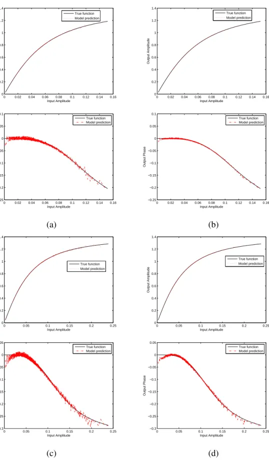
We consider Hammerstein OFDM Systems in which the static nonlinearity described by the HPA (8)-10) is employed using 64-QAM and N = 2048 subcarriers. { Alex, Check A Rayleigh mutlipath fading channel with an exponentially decreasing power delay profile is used. The channel spread is 10 and channel regression factor is set as 3 ???} We used a full OFDM symbol period K =N = 2048 training samples in the joint estimation of the channel impulse coefficient vectorhand the B-spline network parameter vectorθ. The piecewise cubic polynomial (Po = 4) was chosen as the B-spline basis function, and the number of B-spline basis functions was set to eight. The input signals were generated based on the settings of OBO= 5 DB and
OBO = 3 DB respectively. We define Eb as the average power of the input signal xn to the HPA, and No = 2σ2. The empirically determined knot sequences for different HPA operating
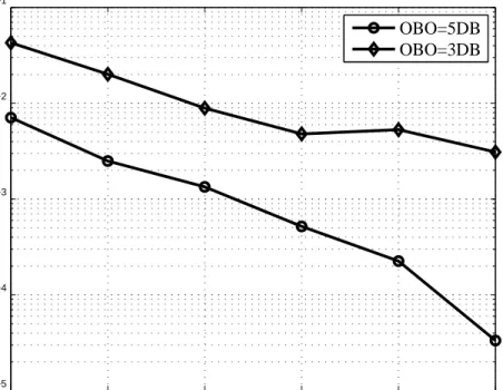
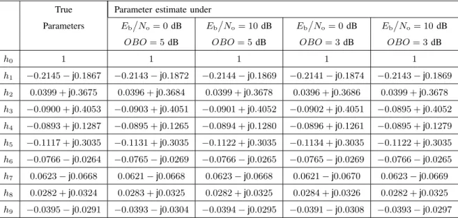
conditions are listed in Table. I. Observe from Table II that the identification of the linear subsystem in the Hammerstein channel was achieved with high accuracy for four conditions. The modeling results of B-spline CV neural network for HPA static nonlinearity are shown in 1, demonstrating that identification algorithm are successful. The BER performance of the proposed nonlinear equalizer of Hammerstein OFDM systems are plotted in Fig. 2, and the proposed nonlinear equalizer is further illustrated using Fig. 3.
0 0.02 0.04 0.06 0.08 0.1 0.12 0.14 0.16 0 0.2 0.4 0.6 0.8 1 1.2 1.4 Input Amplitude Output Amplitude True function Model prediction 0 0.02 0.04 0.06 0.08 0.1 0.12 0.14 0.16 0 0.2 0.4 0.6 0.8 1 1.2 1.4 Input Amplitude Output Amplitude True function Model prediction 0 0.02 0.04 0.06 0.08 0.1 0.12 0.14 0.16 −0.25 −0.2 −0.15 −0.1 −0.05 0 0.05 0.1 Input Amplitude Output Phase True function Model prediction 0 0.02 0.04 0.06 0.08 0.1 0.12 0.14 0.16 −0.25 −0.2 −0.15 −0.1 −0.05 0 0.05 0.1 Input Amplitude Output Phase True function Model prediction (a) (b) 0 0.05 0.1 0.15 0.2 0.25 0 0.2 0.4 0.6 0.8 1 1.2 1.4 Input Amplitude Output Amplitude True function Model prediction 0 0.05 0.1 0.15 0.2 0.25 0 0.2 0.4 0.6 0.8 1 1.2 1.4 Input Amplitude Output Amplitude True function Model prediction 0 0.05 0.1 0.15 0.2 0.25 −0.3 −0.25 −0.2 −0.15 −0.1 −0.05 0 0.05 Input Amplitude Output Phase True function Model prediction 0 0.05 0.1 0.15 0.2 0.25 −0.3 −0.25 −0.2 −0.15 −0.1 −0.05 0 0.05 Input Amplitude Output Phase True function Model prediction (c) (d)
Fig. 1. Comparison of the HPA’s static nonlinearityΨ(•) and the estimated static nonlinearityΨ(b •)under (a) OBO= 5dB,
Eb / No= 0dB; (b) OBO= 5dB,Eb / No= 10dB; (c) OBO= 3dB,Eb / No= 0dB; (d) OBO= 3dB,Eb / No= 10dB;
V. CONCLUSIONS
...
REFERENCES
[1] J. A. C. Bingham, “Multicarrier modulation for data transmission: an idea whose time has come,”IEEE Communications Magazine, Vol. 28, no. 5, pp. 5–14, May 1990.
[2] L. Hanzo, M. M¨unster, B. J. Choi, and T. Keller, OFDM and MC-CDMA for Broadband Multi-User Communications, WLANs, and Broadcasting. Chichester, UK: Wiley, 2003.
[3] A. A. M. Saleh, “Frequency-independent and frequency-dependent nonlinear models of TWT amplifiers,”IEEE Trans. Communications, vol. COM-29, no. 11, pp.1715–1720, Nov. 1981.
TABLE I
EMPIRICALLY DETERMINED KNOT SEQUENCE.
OBO Umin, Vmin Umax, Vmax Knot sequence
5dB -0.15 0.15 -10, -9, -0.3, -0.1, -0.05, -0.02, 0, 0.02, 0.05, 0.1, 0.3, 9, 10 3dB -0.3 0.3 -10, -9, -0.3, -0.15, -0.05, -0.02, 0, 0.02, 0.05, 0.15, 0.3, 9, 10 0 2 4 6 8 10 10−5 10−4 10−3 10−2 10−1 Eb/No (DB)
Bit error rate
OBO=5DB OBO=3DB
TABLE II
IDENTIFICATION RESULTS FORhOF THEHAMMERSTEIN CHANNEL.
True Parameter estimate under Parameters Eb / No= 0 dB Eb / No= 10dB Eb / No= 0 dB Eb / No= 10dB
OBO= 5dB OBO= 5dB OBO= 3dB OBO= 3dB
h0 1 1 1 1 1 h1 −0.2145−j0.1867 −0.2143−j0.1872 −0.2144−j0.1869 −0.2141−j0.1874 −0.2143−j0.1869 h2 0.0399 +j0.3675 0.0396 +j0.3684 0.0399 +j0.3678 0.0396 +j0.3686 0.0399 +j0.3678 h3 −0.0900 +j0.4053 −0.0903 +j0.4051 −0.0901 +j0.4052 −0.0902 +j0.4051 −0.0895 +j0.4052 h4 −0.0893 +j0.1287 −0.0895 +j0.1265 −0.0894 +j0.1280 −0.0896 +j0.1261 −0.0895 +j0.1279 h5 −0.1117 +j0.3035 −0.1131 +j0.3035 −0.1122 +j0.3035 −0.1134 +j0.3035 −0.1122 +j0.3035 h6 −0.0766−j0.0264 −0.0765−j0.0269 −0.0766−j0.0265 −0.0765−j0.0269 −0.0766−j0.0265 h7 0.0623−j0.0668 0.0621−j0.0668 0.0623−j0.0668 0.0621−j0.0670 0.0623−j0.0669 h8 0.0282 +j0.0324 0.0283 +j0.0325 0.0282 +j0.0325 0.0284 +j0.0326 0.0282 +j0.0325 h9 −0.0395−j0.0291 −0.0393−j0.0304 −0.0394−j0.0295 −0.0391−j0.0308 −0.0393−j0.0297
[4] M. Honkanen and S.-G. H¨aggman, “New aspects on nonlinear power amplifier modeling in radio communication system simulations,” inProc. PIMRC’97(Helsinki, Finland), Sept. 1-4, 1997, pp. 844–848.
[5] C. J. Clark, G. Chrisikos, M. S. Muha, A. A. Moulthrop, and C. P. Silva, “Time-domain envelope measurement technique with application to wideband power amplifier modeling,”IEEE Trans. Microwave Theory and Techniques, vol. 46, no. 12, pp. 2531–2540, Dec. 1998.
[6] C.-S. Choi,et al.,“RF impairment models 60 GHz band SYS/PHY simulation,” Document IEEE 802.15-06-0477-01-003c, Nov. 2006.https://mentor.ieee.org/802.15/dcn/06/15-06-0477-01-003c-rf-impairment-models -60ghz-band-sysphy-simulation.pdf
[7] V. Erceg,et al., “60 GHz impairments modeling,” Document IEEE 802.11-09/1213r1, Nov. 2009.
[8] L. Ding, G. T. Zhou, D. R. Morgan, Z. Ma, J. S. Kenney, J. Kim, and C. R. Giardina, “A robust digital baseband predistorter constructed using memory polynomials,”IEEE Trans. Communications, vol. 52, no. 1, pp. 159–165, Jan. 2004.
[9] D. Zhou and V. E. DeBrunner, “Novel adaptive nonlinear predistorters based on the direct learning algorithm,”IEEE Trans. Signal Processing, vol. 55, no. 1, pp. 120–133, Jan. 2007.
[10] M.-C. Chiu, C.-H. Zeng, and M.-C. Liu, “Predistorter based on frequency domain estimation for compensation of nonlinear distortion in OFDM systems,”IEEE Trans. Vehicular Technology, vol. 57, no. 2, pp. 882–892, March 2008.
[11] S. Choi, E.-R. Jeong, and Y. H. Lee, “Adaptive predistortion with direct learning based on piecewise linear approximation of amplifier nonlinearity,”IEEE J. Selected Topics in Signal Processing, vol. 3, no. 3, pp. 397–404, June 2009.
[12] V. P. G. Jim´enez, Y. Jabrane, A. G. Armada, and B. Ait Es Said, “High power amplifier pre-distorter based on neural-fuzzy systems for OFDM signals,”IEEE Trans. Broadcasting, vol.57, no. 1, pp. 149–158, March 2011.
[13] S. Chen, “An efficient predistorter design for compensating nonlinear memory high power amplifier,” IEEE Trans. Broadcasting, vol. 57, no. 4, pp. 856–865, Dec. 2011.
[14] S. Chen, X. Hong, Y. Gong, and C. J. Harris, “Digital predistorter design using B-spline neural network and inverse of De Boor algorithm,”IEEE Trans. Circuits and Systems I, vol. 60, no. 6, pp. 1584–1594, June 2013.
[15] X. Hong, S. Chen, and C. J. Harris, “Complex-valued B-spline neural networks for modeling and inverse of Wiener systems,” Chapter 9 in: A. Hirose, ed.Complex-Valued Neural Networks: Advances and Applications. Hoboken, NJ: IEEE and Wiley, 2012, pp. 209–233.
[16] X. Hong and S. Chen, “Modeling of complex-valued Wiener systems using B-spline neural network,”IEEE Trans. Neural Networks, vol 22, no. 5, pp. 818–825, May 2011.
[17] C. De Boor,A Practical Guide to Splines. New York: Spring Verlag, 1978.
[18] C. J. Harris, X. Hong, and Q. Gan,Adaptive Modelling, Estimation and Fusion from Data: A Neurofuzzy Approach. Berlin: Springer-Verlag, 2002.
[19] E. W. Bai, “An optimal two-stage identification algorithm for Hammerstein-Wiener nonlinear systems,”Automatica, vol. 34, no. 3, pp. 333–338, March 1998. −0.1 −0.05 0 0.05 0.1 −0.1 −0.05 0 0.05 0.1 X −0.2 −0.1 0 0.1 0.2 −0.2 −0.1 0 0.1 0.2 x −0.1 −0.05 0 0.05 0.1 −0.1 −0.05 0 0.05 0.1 estimate X −0.2 −0.1 0 0.1 0.2 −0.2 −0.1 0 0.1 0.2 estimate x
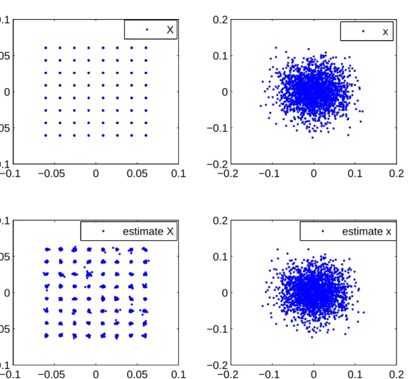
Fig. 3. The illustration of nonlinear equalizer of Hammerstein OFDM systems for one sample OFDM symbol based on
OBO= 5DB,Eb
/
[20] S. Chen, S. McLaughlin, and B. Mulgrew, “Complex-valued radial basis function network, Part I: Network architecture and learning algorithms,”Signal Processing, vol. 35, no. 1, pp. 19–31, Jan. 1994.
[21] S. Chen, S. McLaughlin, and B. Mulgrew, “Complex-valued radial basis function network, Part II: Application to digital communications channel equalisation,”Signal Processing, vol. 36, no. 2, pp. 175–188, March 1994.
[22] A. Uncini, L. Vecci, P. Campolucci, and F. Piazza, “Complex valued neural networks with adaptive spline activation function for digital radio links nonlinear equalization,”IEEE Trans. Signal Processing, vol. 47, no. 2, pp. 505–514, Feb. 1999.
[23] T. Kim and T. Adali, “Approximation by fully complex multilayer perceptrons,” Neural Computation, vol. 15, no. 7, pp. 1641–1666, July 2003.
[24] C.-C. Yang and N. K. Bose, “Landmine detection and classification with complex-valued hybrid neural network using scattering parameters dataset,” IEEE Trans. Neural Networks, vol. 16, no. 3, pp. 743–753, May 2005.
[25] M. B. Li, G. B. Guang, P. Saratchandran, and N. Sundararajan, “Fully complex extreme learning machine,”Neurocomputing, vol. 68, pp. 306–314, Oct. 2005.
[26] A. Hirose,Complex Valued Neural Networks. Berlin: Springer-Verlag, 2006.
[27] S. Chen, X. Hong, C. J. Harris, and L. Hanzo, “Fully complex-valued radial basis function networks: Orthogonal least squares regression and classification,”Neurocomputing, vol. 71, no. 16-18, pp. 3421–3433, Oct. 2008.
[28] T. Nitta, Ed.,Complex-Valued Neural Networks: Utilizing High-Dimensional Parameters. New York: Information Science Reference, 2009.
[29] A. S. Gangal, P. K. Kalra, and D. S. Chauhan, “Inversion of complex valued neural networks using complex back-propagation algorithm,”Int. J. Mathematics and Computers in Simulation, vol. 3, no. 1, pp. 1–8, 2009.
[30] M. Kobayashi, “Exceptional reducibility of complex-valued neural networks,”IEEE Trans. Neural Networks, vol. 21, no. 7, pp. 1060–1072, July 2010.
[31] A. Hirose, ed.,Complex-Valued Neural Networks: Advances and Applications. Hoboken, NJ: John Wiley & Sons, 2012 (in press).
[32] S. A. Billings, “Identification of nonlinear systems – a survey,”IEE Proc. D, vol. 127, no. 6, pp. 272–285, Nov. 1980. [33] I. W. Hunter and M. J. Korenberg, “The identification of nonlinear biological systems: Wiener and Hammerstein cascade
models,”Biological Cybernetics, vol. 55, nos. 2-3, pp. 135–144, 1986.
[34] Y. Zhu, “Estimation of an N-L-N Hammerstein-Wiener model,”Automatica, vol. 38, no. 9, pp. 1607–1614, Sept. 2002. [35] J. Schoukens, J. G. Nemeth, P. Crama, Y. Rolain, and R. Pintelon, “Fast approximate identification of nonlinear systems,”
Automatica, vol. 39, no. 7, pp. 1267–1274, July 2003.
[36] K. Hsu, T. Vincent, and K. Poolla, “A kernel based approach to structured nonlinear system identification part I: algorithms,” in Proc. 14th IFAC Symp. System Identification(Newcastle, Australia), March 29-31, 2006, 6 pages.
[37] K. Hsu, T. Vincent, and K. Poolla, “A kernel based approach to structured nonlinear system identification part II: convergence and consistency,” inProc. 14th IFAC Symp. System Identification(Newcastle, Australia), March 29-31, 2006, 6 pages.
[38] W. Greblicki, “Nonparametric identification of Wiener systems,”IEEE Trans. Information Theory, vol. 38, no. 5, pp. 1487– 1493, Sept. 1992.
[39] A. Kalafatis, N. Arifin, L. Wang, and W. R. Cluett, “A new approach to the identification of pH processes based on the Wiener model,”Chemical Engineering Science, vol. 50, no. 23, pp. 3693–3701, Dec. 1995.
[40] A. D. Kalafatis, L. Wang, and W. R. Cluett, “Identification of Wiener-type nonlinear systems in a noisy environment,”Int. J. Control, vol. 66, no. 7, pp. 923–941, 1997.
[41] Y. Zhu, “Distillation column identification for control using Wiener model,” inProc. 1999 American Control Conference (San Diego, USA), June 2-4, 1999, pp. 3462–3466.
[42] J. C. Gomez, A. Jutan, and E. Baeyens, “Wiener model identification and predictive control of a pH neutralisation process,” IEE Proc. Control Theory and Applications, vol. 151, no. 3, pp. 329–338, May 2004.
[43] I. Skrjanc, S. Blazic, and O. E. Agamennoni, “Interval fuzzy modeling applied to Wiener models with uncertainties,”IEEE Trans. Systems, Man and Cybernetics, Part B, vol. 35, no. 5, pp. 1092–1095, Oct. 2005.
[44] A. Hagenblad, L. Ljung, and A. Wills, “Maximum likelihood identification of Wiener models,”Automatica, vol. 44, no. 11, pp. 2697–2705, Nov. 2008.
[45] S. A. Billings and S. Y. Fakhouri, “Non-linear system identification using the Hammerstein model,”Int. J. Systems Science, vol. 10, no. 5, pp. 567–578, May 1979.
[46] P. Stoica and T. S¨oderstr¨om, “Instrumental-variable methods for identification of Hammerstein systems,”Int. J. Control, vol. 35, no. 3, pp. 459–476, 1982.
[47] A. Balestrino, A. Landi, M. Ould-Zmirli, and L. Sani, “Automatic nonlinear auto-tuning method for Hammerstein modelling of electrical drives,”IEEE Trans. Industrial Electronics, vol. 48, no. 3, pp. 645–655, June 2001.
[48] J. Turunen, J. T. Tanttu, and P. Loula, “Hammerstein model for speech coding,”EURASIP J. Applied Signal Processing, vol. 2003, pp. 1238–1249, Jan. 2003.
[49] S. W. Su, L. Wang, B. G. Celler, A. V. Savkin, and Y. Guo, “Identification and control for heart rate regulation during treadmill exercise,”IEEE Trans. Biomedical Engineering, vol. 54, no. 7, pp. 1238–1246, July 2007.
[50] X. Hong and R. J. Mitchell, “Hammerstein model identification algorithm using Bezier-Bernstein approximation,” IET Control Theory and Applications, vol. 1, no. 1, pp. 1149–1159, April 2007.
[51] X. Hong, R. J. Mitchell, and S. Chen, “Modeling and control of Hammerstein system using B-spline approximation and the inverse of De Boor algorithm,”Int. J. Systems Science, vol. 43, no. 10, pp. 1976–1984, Oct. 2012.
[52] G. Farin,Curves and Surfaces for Computer-Aided Geometric Design: A Practical Guide. Fourth Edition. Boston: Academic Press, 1996.
[53] T. Kavli, “ASMOD – an algorithm for adaptive spline modelling of observation data,” Int. J. Control, vol. 58, no. 4, pp. 947–967, 1993.
[54] M. Brown and C. J. Harris,Neurofuzzy Adaptive Modelling and Control. Hemel Hempstead: Prentice Hall, 1994. [55] Y. Yang, L. Guo, and H. Wang, “Adaptive statistic tracking control based on two-step neural networks with time delays,”
IEEE Trans. Neural Networks, vol. 20, no. 3, pp. 420–429, March 2009.
[56] X. Hong, S. Chen, and C. J. Harris, “Complex-valued B-spline neural networks for modelling and inverse of Wiener systems,” chapter 9 in: A. Hirose, ed.,Complex-Valued Neural Networks: Advances and Applications. Hoboken, NJ: John Wiley & Sons, 2012 (in press).
[57] R. J. Hathaway and J. C. Bezdek, “Grouped coordinate minimization using Newton’s method for inexact minimization in one vector coordinate,”J. Optimization Theory and Applications, vol. 71, no. 3, pp. 503–516, Dec. 1991.
[58] Z. Q. Luo and P. Tseng, “On the convergence of the coordinate descent method for convex differentiable minimization,” J. Optimization Theory and Applications, vol. 72, no. 1, pp. 7–35, Jan. 1991.
[59] B. Igelnik, “Kolmogorov’s spline complex network and adaptive dynamic modeling of data,” in: T. Nitta, Ed., Complex-Valued Neural Networks: Utilizing High-Dimensional Parameters. New York: Information Science Reference: 2009, pp. 56– 78.
[60] M. Scarpiniti, D. Vigliano, R. Parisi, and A. Unicinis, “Flexible blind signal separation in the complex domain,” in: T. Nitta, Ed.,Complex-Valued Neural Networks: Utilizing High-Dimensional Parameters. New York: Information Science Reference, 2009, pp. 284–323.
[61] S. Haykin,Adaptive Filter Theory(2nd Edition). Englewood, NJ: Prentice Hall, 1991.
[62] L. Hanzo, S. X. Ng, T. Keller, and W. Webb,Quadrature Amplitude Modulation: From Basics to Adaptive Trellis-Coded, Turbo-Equalised and Space-Time Coded OFDM, CDMA and MC-CDMA Systems. Chichester, UK: John Wiley, 2004. [63] J. G. Proakis,Digital communications(4th edition). McGraw-Hill, 2000.