Hyperparameter Selection of One-class Support Vector Machine by
Self-adaptive Data Shifting
Siqi Wang, Qiang Liu, En Zhu, Fatih Porikli, Jianping Yin
PII:
S0031-3203(17)30356-4
DOI:
10.1016/j.patcog.2017.09.012
Reference:
PR 6279
To appear in:
Pattern Recognition
Received date:
13 April 2017
Revised date:
29 June 2017
Accepted date:
6 September 2017
Please cite this article as: Siqi Wang, Qiang Liu, En Zhu, Fatih Porikli, Jianping Yin, Hyperparameter
Selection of One-class Support Vector Machine by Self-adaptive Data Shifting,
Pattern Recognition
(2017), doi:
10.1016/j.patcog.2017.09.012
This is a PDF file of an unedited manuscript that has been accepted for publication. As a service
to our customers we are providing this early version of the manuscript. The manuscript will undergo
copyediting, typesetting, and review of the resulting proof before it is published in its final form. Please
note that during the production process errors may be discovered which could affect the content, and
all legal disclaimers that apply to the journal pertain.
ACCEPTED MANUSCRIPT
Hihglights
• We propose a novel self-adaptive data shifting based method for one-class SVM (OCSVM) hyperparameter selection, which has a significant influ-ence on OCSVM performance.
• The proposed method is able to generates a controllable number of high-quality pseudo outlier data around target data by efficient edge pattern detection and a “negative shifting” mechanism, which can effectively reg-ulate the OCSVM decision boundary for an accurate target data descrip-tion. Meanwhile, negative shifting soundly addresses two major difficul-ties of previous pseudo outlier generation based hyperparameter selection methods.
• The proposed method also generates pseudo target data for OCSVM model validation on target class by a “positive shifting” mechanism, which provides an efficient alternative to the time-consuming cross-validation or leave-one-out (LOO) process. More importantly, positive shifting can en-courage robustness to noise in the given target data during hyperparam-eter selection, by generating non-noise pseudo target data for validation from original noise.
• The proposed method is able to yield superior performance when com-pared with other state-of-the-art OCSVM hyperparameter selection meth-ods, on both synthetic 2-D datasets and various benchmark datasets.
• Unlike many previous methods that introduce additional hyperparameters into OCSVM hyperparameter selection, the proposed method is fully au-tomatic and self-adaptive, leaving no additional hyperparameter for users to tune. Besides, the application of the proposed method is not restricted to certain kernel functions like Gaussian kernel.
ACCEPTED MANUSCRIPT
Hyperparameter Selection of One-class Support Vector
Machine by Self-adaptive Data Shifting
Siqi Wanga,∗, Qiang Liua, En Zhua, Fatih Poriklib, Jianping Yina,c aCollege of Computer,
National University of Defense Technology, Changsha, 410073, China bCollege of Engineering and Computer Science (CECS), Australian National University, Canberra, ACT 2601, Australia
cState Key Laboratory of High Performance Computing, National University of Defense Technology, Changsha, 410073, China
Abstract
With flexible data description ability, one-class Support Vector Machine (OCSVM) is one of the most popular and widely-used methods for one-class classification (OCC). Nevertheless, the performance of OCSVM strongly relies on its hyper-parameter selection, which is still a challenging open problem due to the absence of outlier data. This paper proposes a fully automatic OCSVM hyperparam-eter selection method, which requires no tuning of additional hyperparamhyperparam-eter, based on a novel self-adaptive ”data shifting” mechanism: Firstly, by efficient edge pattern detection (EPD) and ”negatively” shifting edge patterns along the negative direction of estimated data density gradient, a constrained number of high-quality pseudo outliers are self-adaptively generated at more desirable locations, which readily avoids two major difficulties in previous outlier genera-tion methods. Secondly, to avoid time-consuming cross-validagenera-tion and enhance robustness to noise in the given training data, a pseudo target set is generated for model validation by ”positively” shifting each given target datum along the positive direction of data density gradient. Experiments on synthetic and benchmark datasets demonstrate the effectiveness of the proposed method. Keywords: one-class SVM, hyperparameter selection, data shifting
∗Corresponding author. Tel.: +86 18670707447.
ACCEPTED MANUSCRIPT
1. Introduction
One-class classification (OCC) [1] describes training data from a single class (called ”target class”) as a normalcy model and aims to detect data from any other class (called ”outlier class”) as outliers. OCC has numerous applications, especially when training data from outlier class are hard or even impossible to obtain. To deal with OCC, existing methods basically fall into three categories: (i)Density based methods. Density based methods, like one-class Gaussian Mix-ture Model (OCGMM) [2] and Parzen density estimation [3], estimate the den-sity of the target class and detect data in low-denden-sity area as outliers. (ii) Reconstruction based methods. Reconstruction methods, such as auto-encoder network [4], assume that target data can be reconstructed by a network with low reconstruction error, while outliers cannot. (iii)Boundary based methods. Boundary based methods, such as One-class Support Vector Machine (OCSVM) [5] and Support Vector Data Description (SVDD) [6], are able to learn a tight and smooth boundary that encloses target data by introducing non-linear ker-nel tricks, which makes boundary based methods particularly popular in OCC. As a prevalent boundary based OCC method, OCSVM has been studied and applied actively in numerous realms of academic research and industrial appli-cations, such as fault detection [7], video abnormal event detection [8], media classification [9], network intrusion detection [10], video summarization [11], etc. Besides, another representative OCC method SVDD is shown to be equivalent to OCSVM when stationary kernel is used [5] (e.g. standard Gaussian kernel). However, a pivotal issue to apply OCSVM is the hyperparameter selection, which has a significant influence on its performance. To be more specific, with the standard Gaussian kernel, two hyperparameters of OCSVM need to be prop-erly tuned: the regularization coefficient ν and the Gaussian kernel width σ
(details will be reviewed in Sec. 2.1). ν controls the upper bound of rejected target data [5], which is often tuned to reject noise in the target data during training OCSVM, while σ controls the smoothness of decision boundary. To illustrate this, we show the decision boundary of OCSVM with different
hy-ACCEPTED MANUSCRIPT
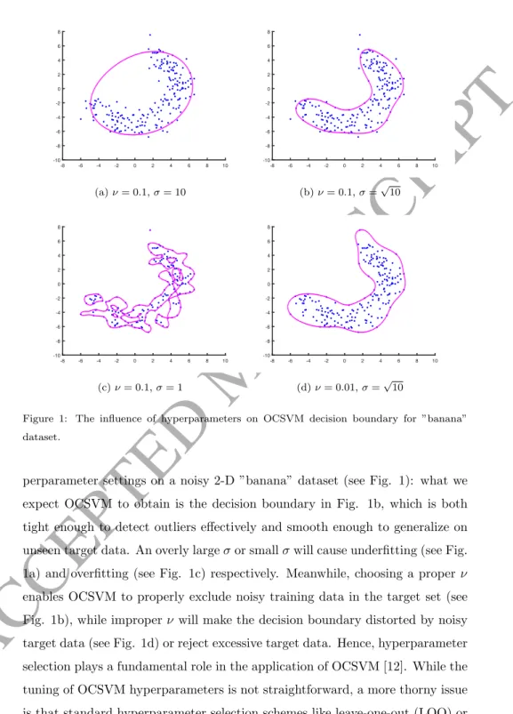
-8 -6 -4 -2 0 2 4 6 8 10 -10 -8 -6 -4 -2 0 2 4 6 8 (a)ν= 0.1,σ= 10 -8 -6 -4 -2 0 2 4 6 8 10 -10 -8 -6 -4 -2 0 2 4 6 8 (b)ν= 0.1,σ=√10 -8 -6 -4 -2 0 2 4 6 8 10 -10 -8 -6 -4 -2 0 2 4 6 8 (c)ν= 0.1,σ= 1 -8 -6 -4 -2 0 2 4 6 8 10 -10 -8 -6 -4 -2 0 2 4 6 8 (d)ν= 0.01,σ=√10Figure 1: The influence of hyperparameters on OCSVM decision boundary for ”banana” dataset.
perparameter settings on a noisy 2-D ”banana” dataset (see Fig. 1): what we expect OCSVM to obtain is the decision boundary in Fig. 1b, which is both tight enough to detect outliers effectively and smooth enough to generalize on unseen target data. An overly largeσor smallσwill cause underfitting (see Fig. 1a) and overfitting (see Fig. 1c) respectively. Meanwhile, choosing a properν
enables OCSVM to properly exclude noisy training data in the target set (see Fig. 1b), while improperν will make the decision boundary distorted by noisy target data (see Fig. 1d) or reject excessive target data. Hence, hyperparameter selection plays a fundamental role in the application of OCSVM [12]. While the tuning of OCSVM hyperparameters is not straightforward, a more thorny issue is that standard hyperparameter selection schemes like leave-one-out (LOO) or
ACCEPTED MANUSCRIPT
cross-validation will be problematic for OCC due to the absence of data from outlier class, and the model error on outlier class can longer be obtained directly [12, 13]. As a result, hyperparameter selection of OCSVM remains a challeng-ing open problems and many attempts have been made to tackle this problem, which will be reviewed in Sec. 2.2.
In this paper, we enable fully automatic OCSVM hyperparameter selection by a novel self-adaptive data shifting (SDS) based method, which consists of two contributions: Firstly, based on an efficient edge pattern detection (EPD) method, pseudo outliers are generated by ”negatively” shifting the detected edge patterns for model error estimation on outlier class. The proposed method can generate a controllable number of high-quality deterministic pseudo outliers at more desirable locations in the data space, which can effectively regulate the decision boundary of OCSVM for a more accurate target data description. More importantly, negative shifting avoids two major difficulties in previous outlier generation methods (discussed in Sec. 2.2). Secondly, a pseudo target data set is generated by an efficient ”positive shifting” mechanism for model validation on target class, which can avoid time-consuming cross-validation. The generated pseudo target data can perfectly preserve the original target data distribution, so as to soundly evaluate the generalization performance on target class and prevent overfitting. Meanwhile, it can enhance the robustness to noise in the given target data by generating normal pseudo target data from noise for model validation. Unlike many previous methods, both negative and positive shifting are self-adaptive and leave no additional hyperparameter for users to tune dur-ing OCSVM hyperparameter selection. Experimental results demonstrate that the proposed method enables OCSVM to accurately describe target data with complex data distributions and achieve satisfactory OCC performance.
The rest of paper is organized as follows: Sec. 2 revisits the basics of OCSVM (Sec. 2.1) and then briefly reviews existing hyperparameter selection methods for OCSVM (Sec. 2.2). Sec. 3 presents the proposed data shifting based OCSVM hyperparameter selection method in detail. Sec. 4 reports the exper-imental results of the proposed method on both synthetic datasets and
bench-ACCEPTED MANUSCRIPT
mark datasets in comparison with existing OCSVM hyperparameter selection methods. Sec. 5 concludes this paper.
2. Related Work
2.1. One-class Support Vector Machine (OCSVM)
Before we discuss the hyperparameter selection of OCSVM, it is neces-sary to review the basics of OCSVM first. As an extension of the standard binary SVM, Sch¨olkopf et al. [5] proposed OCSVM to handle OCC prob-lems. Formally, suppose that the target data to be described by OCSVM is Xtarget={x1,x2,· · ·,xN}, and an implicit mappingφ(·) that can map target
data from their original feature space to a new feature spaceH. OCSVM intends to seek such a hyper-plane Π inH: the hyper-plane Π :wT·φ(x)−ρ= 0 (wis
a normal vector of Π) has the largest distance to the origin, while all mapped target dataφ(xi) lie at the opposite side of hyper-plane to the origin. This goal
can be formulated as the following primal optimization problem:
min w,ξ,ρ 1 2||w|| 2+ 1 νN N X i=1 ξi−ρ s.t. wT ·φ(xi)−ρ+ξi≥0, ξi≥0, ∀i (1)
where ν is the regularization coefficient mentioned in Sec. 1, which trades off model complexity and training error, andξiis the slack variable that enables
OCSVM to have soft matgin so as to exclude some noisy training data. It is proved that, hyperparameter ν controls the upper bound of the training data that are excluded by the decision boundary of OCSVM [5]. Since the mapping
φ(·) is usually implicit, the above optimization problem is usually solved by its dual form: max α − 1 2 N X i,j=1 αiαjK(xi,xj) s.t. N X i=1 αi= 1, 0≤αi≤ 1 νN,∀i (2)
ACCEPTED MANUSCRIPT
whereK(xi,xj) =φ(xi)T·φ(xj) is the inner product of mapped data, while
αiis the dual variable. In practice, one usually directly specifies kernel function
K(xi,xj) instead of the mappingφ(x), which may be indefinite, and Gaussian
kernel K(xi,xj) = exp(−||xi−xj|| 2
σ2 ) is usually the standard choice (σ is the
Gaussian kernel width). With selected kernel function and its hyperparameter, the above dual optimization problem can be solved as a quadratic programming problem. Having solvedαiby the dual optimization problem,ρcan be obtained
by choosing anyxithat its correspondingαisatisfies 0< αi< νN1 and calculate
ρ=PNj=1αjK(xi,xj). In the meantime, anyxithat has a correspondingαi>0
is called a support vector, which supports the decision boundary of OCSVM. An incoming new datumxt is determined as an outlier if it satisfies:
f(xt) =
X
αi>0
αiK(xt,xi)−ρ <0 (3)
In this paper, we will focus on the hyperparameter selection of standard Gaussian kernel based OCSVM, but the applicability of the proposed method is not limited to Gaussian kernel. Existing methods on OCSVM hyperparameter selection are reviewed in next section below.
2.2. Existing OCSVM Hyperparameter Selection Methods
Since the very beginning, researchers have noticed the dramatic influence of hyperparameters on the performance of OCSVM/SVDD. Sch¨olkopf et al. [5] analyzed the influence of hyperparameter ν and σ from a theoretical view, but did not provide specific guidelines to their selection. Afterwards, a host of methods are proposed and we roughly classify them into two categories:
(1)Pseudo outlier generation based methods. The motivation of this type of methods is straightforward as they intend to tackle the essence of OCC problem: the absence of outlier data. An early attempt is Fan et al. [14], who replaced the feature value that appears most frequently with a randomly chosen value to generate artificial anomalies. However, this method can only deal with feature with discrete values. Taxet al. [1] studied an intuitive solution: generating uni-formly distributed random outliers in the hyper-cube that encloses the target
ACCEPTED MANUSCRIPT
data to guide hyperparameter selection, and they further improved the hyper-cube into a hyper-sphere to better fit the target data [12]. Unfortunately, as [12] pointed out by themselves, such simple random outlier generation faces two major difficulties: Firstly, outliers are not guaranteed to be generated at desir-able locations due to randomness. [6] discovered that pseudo outliers inside or overly far from the target data are not contributing, and they may even lead to selecting poor hyperparameters. Secondly, as a small number of randomly located outliers cannot deliver an accurate error estimation on outlier class, such methods require generating massive random outliers to fill in the entire data space, so as to yield a relatively good estimation of the model error on outlier class. [12] pointed out that the number of pseudo outliers required for filling can grow exponentially as the feature dimension increases, which makes it particularly difficult to know the exact number of outliers sufficient for a good outlier error estimation. In other words, such methods actually introduce an-other non-intuitive hyperparameter to specify: the amount of generated outliers
No. Some other improved outlier generation methods are proposed: Denget al.
[15] proposed a ”skewness” based outlier generation method, which generates outliers by randomly ”skewing” each target datum from its original location. However, the degree of skewnessαis another sensitive hyperparameter for users to specify. Banhalmi et al. [16] detect boundary points and generate outliers by a transformation between each given datum and its nearest boundary point, but it requires training one SVM for each datum for boundary detection, which is extremely expensive. Besides, it introduces two additional hyperparameters
distandcurv. Desiret al. [17] improved pseudo outlier distribution by using a complementary histogram to indicate the probability of outlier generation. In addition, Tax et al. [13] proposed a ”consistency” based method to avoid the difficulties of explicit outlier generation. It starts with the most underfitting OCSVM model, and gradually tightens the model boundary until the model no longer satisfies the defined ”consistency” criteria, which is set under an implicit uniform outlier distribution assumption. Nevertheless, the performance of this method is actually very sensitive to the ”consistency” criteria, which depends
ACCEPTED MANUSCRIPT
on the threshold of variance, a tunable hyperparameter.
(2)Heuristics based methods. Due to the difficulties of pseudo outlier gen-eration, heuristics based OCSVM hyperparameter tuning has gained increasing popularity over the years. Generally speaking, heuristics based methods assume that good hyperparameters of OCSVM typically satisfy some intuitive observa-tions or empirical prior knowledge, and some corresponding heuristic rules are adopted to provide guidance on OCSVM hyperparameter selection. Specifically, Evangelistaet al. [18] proposed to select goodσ by maximizing the ratio be-tween the variance and average value of kernel matrix’s off-diagonal elements. Khazai et al. [19] proposed to determine σ by the maximal distance between target data and target data number. Xiao et al. [7] proposed two heuristics to tune σ based on maximal-minimal distance between target data and the statistics of distance to nearest neighbor, respectively. However, all methods above need to pre-specifyν, which can sometimes be difficult. Wanget al. [20] proposed a method named Min#SV+MaxL to tune both ν and σ based on a trade-off between minimizing support vector number and maximizing objective value. Xiao et al. [21] put forward an interesting method named MIES: by calculating normalized distance (ND) from target data to OCSVM’s decision boundary, MIES is based on the following observation: good OCSVM hyper-parameters can maximize the difference between ND of data inside the target set (called ”interior patterns”) and the ND of data on the boundary area of the target set (called ”edge patterns”). A more recent work by Ghafooriet al. [22] proposed to estimateνandσ efficiently and unsupervisedly by seeking the ”knee-point” with the largest curvature in the sorted density measure of target data and a revised Duplex Max-margin Model Selection (RDMMS) method. Heuristics based methods can avoid the difficulties of pseudo outlier generation, but they sometimes perform poorly since the underlying observations do not hold. In addition, the application of heuristics based methods are often limited to certain kernel functions like Gaussian kernel.
ACCEPTED MANUSCRIPT
3. Methodology
As we discussed in Sec. 2.2, existing outlier generation based hyperparame-ter selection methods are faced with two major unsolved difficulties, and usually introduce additional hyperparameters that need to be specified by users. This paper proposes a self-adaptive OCSVM hyperparameter selection method based on a novel ”data shifting” mechanism, which can readily avoid the aforemen-tioned difficulties in previous outlier generation methods and leave no tuning of additional hyperparameter to users.
3.1. Self-adaptive Data Shifting
Our hyperparameter selection method for OCSVM based on self-adaptive data shifting is composed of three components: (1) Pseudo outlier data gen-eration by negative shifting. By employing edge pattern detection (EPD) [23] method and calculating the negative data density gradient [24], we develop a new ”negative shifting” mechanism to obtain pseudo outlier data by shifting the detected edge patterns of the target data along the direction of negative data gradient. (2) Pseudo target data generation by positive shifting. With the calculated data density gradient of each given target datum, we develop a novel ”positive shifting” mechanism to generate pseudo target data by shifting each target datum slightly along the direction of positive data density gradient. (3) Grid search. With the generated pseudo outlier and target data as validation data, we use grid search to select good hyperparameters for OCSVM. The pro-posed positive shifting and negative shifting mechanism will be introduced in detail by Sec. 3.2 and Sec. 3.3 respectively, and the whole algorithm will be shown by Sec. 3.4.
3.2. Pseudo Outlier Data Generation by Negative Shifting 3.2.1. Edge Pattern Detection (EPD)
The proposed method is inspired by the working mechanism of SVM [25]: the decision boundary of SVM can be supported only using the exterior patterns in each data class, which are called support vectors. Motivated by this, we discover
ACCEPTED MANUSCRIPT
that it is actually unnecessary to generate massive random outliers to fill in the entire data space like [12]. To regulate the OCSVM decision boundary for an accurate target data description, we can simply generate a small number of high-quality pseudo outliers that tightly surround the domain of target data, serving as pseudo ”supports” from the outlier class. Thus, a novel solution is proposed to generate such high-quality outliers: we shift the data at the exterior surface of target class (denoted as ”edge patterns”) outwards into pseudo outliers (see Fig. 3a), which is called ”negative shifting” and will be discussed in the next section. Before we generate outliers by negative shifting, we will show how to locate the edge patterns at the exterior of target class efficiently in the first place, which is called edge pattern detection (EPD).
ni
vij Tangent plane
Data exterior surface
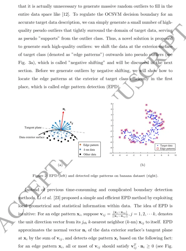
k-nn data Other data Edge pattern (a) -8 -6 -4 -2 0 2 4 6 8 10 -10 -8 -6 -4 -2 0 2 4 6 8 Target data Edge patterns (b) Figure 2: EPD (left) and detected edge patterns on banana dataset (right).
Instead of previous time-consuming and complicated boundary detection methods, Liet al. [23] proposed a simple and efficient EPD method by exploiting local geometrical and statistical information within data. The idea of EPD is intuitive: For an edge patternxi, supposevij = ||(xxii−−xxijij)||, j= 1,2,· · ·k, denotes
the unit direction vector from itsjthk-nearest neighbor (k-nn)xijto itself. EPD
approximates the normal vectorni of the data exterior surface’s tangent plane
atxiby the sum ofvij, and detects edge patternxibased on the following fact:
ACCEPTED MANUSCRIPT
2a). A detailed EPD algorithm is shown in Algorithm 1, in which the indicator function I(·) = 1 if the statement in the bracket is true, otherwise I(·) = 0. It should be noted that two parameters of the EPD algorithm, the number of nearest neighborskand the decision thresholdT, have been thoroughly studied by Li et al., and we simply fix them as the recommended values from [23] in Algorithm 1. Therefore, the EPD process does not require user to specify any parameter. As an illustration, EPD is performed on the banana dataset and the results are displayed in Fig. 2b, which shows EPD can effectively detect the edge patterns of a given target data set.
Algorithm 1:EPD Algorithm.
Input: Taregt datasetXtarget={x1,x2,· · ·,xN}
Output: Edge pattern setXedge
1 calculatek=d5 log10Ne; 2 set thresholdT = 0.1; 3 setXedge=∅;
4 fori= 1toN do
5 calculatek-nn direction vectorvij= ||(xxii−−xxijij)||, j= 1,2,· · ·k;
6 approximate normal vectorni=Pkj=1vij;
7 calculateθij=vTij·ni, j= 1,2,· · ·k; 8 calculateli= 1kPkj=1I(θij ≥0); 9 if li≥1−T then 10 Xedge=Xedge∪xi; 11 returnXedge; 3.2.2. Negative Shifting
With detected edge patterns, we will introduce how to shift them into pseudo outliers to regulate the OCSVM decision boundary and provide guidance on selecting good hyperparameters. Since the edge patterns are shifted ”away” from the target data, this process is called ”negative shifting” (see Fig. 3a).
ACCEPTED MANUSCRIPT
ls
Data exterior surface
Pseudo outlier Other data Edge pattern −∇𝑝(𝐱) k-nn data (a) -8 -6 -4 -2 0 2 4 6 8 10 -10 -8 -6 -4 -2 0 2 4 6 8 Target data Edge pattern Pseudo outlier (b)
Figure 3: Negative shifting (left) and pseudo outliers on banana dataset (right).
To generate high-quality outliers, two key elements need to be determined for negative shifting: the shifting direction and shifting magnitude. We will discuss the shifting direction first. Theoretically, we should shift edge patterns along the direction of target data density’s negative gradient, in which the target data density drops at the fastest rate. In other words, it is the easiest direction for edge patterns to be shifted to the nearby region that has no existence of target data and become valid high-quality pseudo outliers. Formally speaking, with the density of target data at a pointxdenoted asp(x), the ideal shifting direction is−∇p(x). We follow the method in [24] (p. 534) to derive the approximation of−∇p(x): for any givenx, we define a sufficiently small local region centered atxwith radiusr: L(x) ={y|kx−yk2≤r2}. As the data density atyisp(y),
the total amount of data covered byL(x) is:
a=
Z
L(x)
p(y)dy (4)
The direction vector from the centerxto a pointyinL(x) is (y−x). The expectation of such direction vectors inL(x) is:
E{(y−x)|L(x)} ∼=
Z
L(x)
(y−x)p(y)
ACCEPTED MANUSCRIPT
AsL(x) is a small enough local region centered atx, we can approximatea
by the equation below:
a=
Z
L(x)
p(y)dy∼=p(x)u (6)
whereuis the volume ofL(x). By Taylor expansion, we havep(y)∼=p(x) + (y−x)T∇p(x). Therefore, with Taylor expansion ofp(y) and Eq. 6, Eq. 5 can
be transformed into: E{(y−x)|L(x)} ∼= Z L(x) (y−x)1 udy+ Z L(x) (y−x)(y−x)T1 udy ∇p(x) p(x) (7)
Since L(x) is a symmetric region, we have RL(x)(y−x)1
udy = 0. By the
conclusion from [24] (Appendix B.6), Eq. 7 can be converted to:
E{(y−x)|L(x)} ∼= Z L(x) (y−x)(y−x)T1 udy ∇p(x) p(x) = r2 D+ 2 ∇p(x) p(x) (8)
whereDis the dimension ofx. Finally, with the scalar value D+2
r2 p(x),s,
the desired shifting direction−∇p(x) can be approximated by:
−∇p(x)∼=sE{(x−y)|L(x)} ∼= s k k X j=1 (x−xj) (9)
wherexj is thejth k-nn ofx. Eq. 9 suggests that the negative data density
gradient direction can be approximated by the direction vectors from the k -nn data of x to itself. However, the approximation in Eq. 9 has a practical problem: since the given real-world target data near the data exterior surface are usually non-uniform and noisy, the estimated−∇p(x) is often dominated by some noisyk-nn with very large magnitudekx−xik. To enhance the robustness to k-nn noise, we adopt the same solution in [16, 23] to normalize the k-nn direction vector by its magnitude. This makes the estimated −∇p(x) exactly coincide with the normal vectorn calculated during EPD, which facilitates us
ACCEPTED MANUSCRIPT
to determine both edge patterns and their shifting directions by EPD:
−∇p(x)∼=n= k X j=1 x−xj kx−xjk (10)
where the scalar sk in Eq. 9 is dropped since we are only interested in the di-rection of−∇p(x). The second consideration is the negative shifting magnitude
lns. A proper shifting magnitude is vital: overly largelnswill generate outliers
that cannot regulate the OCSVM decision boundary, while overly smalllnswill
make outliers too close to target data, which may lead to overfitting decision boundary. However, it is not easy to manually set a good shifting magnitude for different target data. To automatically determine a properlns, it is assumed
that a functioning pseudo outlier has alnsthat is equal to the average distance
ofk-nn data to this edge pattern. The assumption is intuitive: it ensures the generated outlier to be no further than the furthestk-nn data of an edge pattern, which avoids an overly distant outlier, while it also ensures that the generated outlier to be no closer than some k-nn data of an edge pattern, which avoids an overly close outlier, i.e. minjkx−xjk ≤lns≤maxjkx−xjk(see Fig. 3a).
As we mentioned above, thek-nn of a single edge pattern is often noisy, so we average the meank-nn distance of all edge patterns as a more robust ¯lns:
¯ lns= 1 |Xedge| X xi∈Xedge 1 k k X j=1 kxi−xijk (11)
Finally, we can generate a pseudo outliers set by negative shifting as follows:
Xoutlier={x(oi)|x(oi)=xi+ ni
knik·¯lns,∀xi∈Xedge} (12)
Since bothk-nn distance andnihave been calculated during EPD, the
lier generation calls for minimal computation. We visualize the generated out-liers for banana dataset in Fig. 3b as an example. Compared with previous outlier generation methods, the pseudo outlier data generated above enjoy the advantages below: (1) As Fig. 3b shows, the generated pseudo outliers can compactly surround the target data domain while keeping a moderate distance
ACCEPTED MANUSCRIPT
to target data, which soundly addresses the first difficulty discussed in Sec. 2.2: generating good outliers at desirable locations. (2) Since each pseudo outlier is yielded by negatively shifting the detected edge patterns, the number of gen-erated pseudo outlier is always smaller or equal to the number of target data, i.e. |Xoutlier|=|Xedge| ≤ |Xtarget|, which avoids the second difficulty to
gener-ate exponentially-growing pseudo outliers in the high-dimensional space. (3) A prominent merit of the proposed negative shifting process is self-adaptiveness: it requires no tuning of additional hyperparameters by users. Both the shifting direction and magnitude are automatically derived from the target data without human effort, and the number of generated pseudo outliers needs not to be spec-ified as well. In addition, it is worth noting the generated outliers are only for model validation purpose, i.e. they are not used as training data. Using those outliers as negative training data will make the decision boundary shift towards the outliers to cover redundant marginal space and accepts more outliers. 3.3. Pseudo Target Data Generation by Positive Shifting
Having obtained pseudo outliers to estimate the error on outlier class, we also need to estimate the error on target class, so as to preserve generalization performance and avoid an overfitting model like Fig. 1c. To estimate error on target class, leave-one-out (LOO) or cross-validation (CV) are usually adopted, which often leads to intolerable long hyperparameter selection time [6, 22]. The problem is further exacerbated when dealing with a relatively large number of training data. For example, since the training complexity of OCSVM is usually
O(N3) [5], applying a standard 10-fold CV to validating a certain
hyperparame-ter combination requires roughly a complexity ofO(10×(9
10N)3)≈O(7.29N3).
However, if we can generate a separated pseudo target data set as the valida-tion set, it only requires training OCSVM once with all given target data, i.e. a complexity ofO(N3), which can be much faster than usual CV. To illustrate
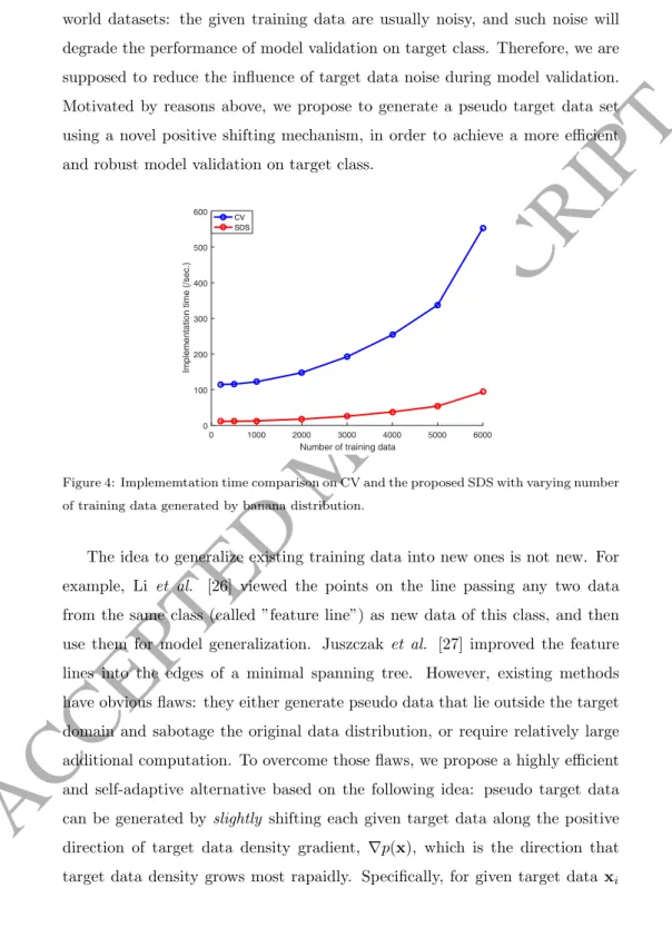
this, we compare the implementation time of 10-fold CV and the proposed SDS method with a separated pseudo target set for validation when the number of training data varies in Fig. 4. Besides, there is another problem with
real-ACCEPTED MANUSCRIPT
world datasets: the given training data are usually noisy, and such noise will degrade the performance of model validation on target class. Therefore, we are supposed to reduce the influence of target data noise during model validation. Motivated by reasons above, we propose to generate a pseudo target data set using a novel positive shifting mechanism, in order to achieve a more efficient and robust model validation on target class.
0 1000 2000 3000 4000 5000 6000
Number of training data
0 100 200 300 400 500 600
Implementation time (/sec.)
CV SDS
Figure 4: Implememtation time comparison on CV and the proposed SDS with varying number of training data generated by banana distribution.
The idea to generalize existing training data into new ones is not new. For example, Li et al. [26] viewed the points on the line passing any two data from the same class (called ”feature line”) as new data of this class, and then use them for model generalization. Juszczak et al. [27] improved the feature lines into the edges of a minimal spanning tree. However, existing methods have obvious flaws: they either generate pseudo data that lie outside the target domain and sabotage the original data distribution, or require relatively large additional computation. To overcome those flaws, we propose a highly efficient and self-adaptive alternative based on the following idea: pseudo target data can be generated byslightly shifting each given target data along the positive direction of target data density gradient, ∇p(x), which is the direction that target data density grows most rapaidly. Specifically, for given target data xi
ACCEPTED MANUSCRIPT
and theirk-nn neighborsxij, j = 1,2,· · ·, k, the pseudo target data setX
0 target is generated by: X0target={x (i) t |x (i) t =xi+ ∇p(xi) k∇p(xi)k ,xmin +ij −xi · ∇p(xi) k∇p(xi)k ,∀xi∈Xtarget} (13) whereh·idenotes inner product andxmin +ij is defined by:
xmin +ij = argmin xij∈Λ+i { ∇p(xi) k∇p(xi)k,xij−xi } (14)
where Λ+i is the set ofk-nn data ofxi that satisfy
D ∇p(xi)
k∇p(xi)k,xij−xi E
>0 (Λ−i can be defined as the opposite), and∇p(xi) can be estimated by Eq. 10
as we discussed in last section. For an intuitive interpretation, we show the process of positive shifting by Fig. 5a: the termD ∇p(xi)
k∇p(xi)k,xij−xi E
represents the projection length of (xij−xi) on the direction of∇p(xi). Eq. 13 actually
indicates that a new pseudo target datum is generated by thek-nn datum that has the smallest positive projection distance to the original target datum (the red point in Fig. 5a), which explains the name ”positive shifting”.
𝜦𝒊+
Candidate data Target data Pseudo target data
∇𝑝(𝐱) k-nn data Nearest k-nn data (a) -8 -6 -4 -2 0 2 4 6 8 10 -10 -8 -6 -4 -2 0 2 4 6 8 Target data Pseudo target data Noise Pseudo data gen. by noise
(b) Figure 5: Positive shifting (left) and pseudo target data of banana (right).
We will explain why the generated pseudo target data have very high confi-dence to be data from the target class: since the pseudo target data are
gener-ACCEPTED MANUSCRIPT
ated by shifting each given target datum along the direction∇p(xi) by a small
distance (we will explain why the distance is small later), we have two good rea-sons to believe that the generated data belong to the target class: Firstly, it is on the direction that target data density rises most rapidly (∇p(xi)); Secondly,
if a given target datum is not noise, the generated datum will be guaranteed to stay very closely to the original target datum. To prove this, suppose the nearestk-nn data toxi in the set Λ+i is denoted byxnij+(denoted by the orange
point in Fig. 5a, andxnij−is similarly defined), the generated datum (red point)
will be strictly confined to the small region centered atxiwith radiuskxnij+−xik
(denoted by the orange dashed cirlce in Fig. 5a), which can be proved easily by the definition ofxmin +ij in Eq. 14:
kx(ti)−xik= xmin +ij −xi, ∇p(xi) k∇p(xi)k ≤ xnij+−xi, ∇p(xi) k∇p(xi)k ≤ kxnij+−xik (15) By Eq. 15, for edge patterns on convex surface of the target data (li = 1
in EPD, e.g. the edge pattern shown in Fig. 2a), we have kxn+
ij −xik =
minjkxij−xikbecause Λ+i contains allk-nn data, which yields: kx(ti)−xik ≤min
j kxij−xik (16)
For edge patterns on non-convex surface and target data that are not edge patterns (li<1), since the vector∇p(xi) points to the region with denser data, kxnij+−xik ≤ kxnij−−xik is usually satisfied (though not always), Eq. 16 can often be satisfied as well. Therefore, ifxi is not noise, x(ti) stays very closely
to xi, i.e. often closer than the nearest neighbor ofxi. In the meantime, by
definition of Λ+i , we have: kx(ti)−xik= xmin +ij −xi, ∇p(xi) k∇p(xi)k >0 (17)
Consequently, eachx(ti) is definitely different from the givenxi by Eq. 17,
ACCEPTED MANUSCRIPT
in most cases is less than the distance to xi’s nearest neighbor). Thus, the
proposed pseudo target data generation method enjoys the following merits: (1) Each pseudo target datum, if not noise, is generated through shifting the original target datum off its original location by a provable small distance, so the generated pseudo target data can perfectly preserve the data distribution of the given target data (e.g. see the generated pseudo target data on banana dataset in Fig. 5b). Thus, the generated pseudo target data can provide a favorable estimation on the model error of target class to prevent overfitting. (2) Like negative shifting, the proposed positive shifting can generate pseudo target data in an efficient and self-adaptive manner. As Eq. 13 suggests, the
k-nn and data density gradient∇p(x) can both be obtained during the EPD process in Sec. 3.2.1, and little additional computation is needed. Meanwhile, the positive shifting process leaves no hyperparameter for users to tune, which is self-adaptive as well. (3) More importantly, the designed positive shifting scheme can encourage robustness to noise in the given target data by generating noise-free pseudo target data for model validation. To encourage a smooth and tight boundary, noise should be encouraged to be excluded by OCSVM decision boundary. The proposed positive shifting enables training data noise to generate a normal pseudo target datum that is not noise by attracting it back to data-dense region (see Fig. 6). In this way, an error of noise is no longer regarded as an error on target class during model validation, which enhances the robustness to noise. As an example, in Fig. 5b, the training data noise of banana dataset (in blue triangle) generates a normal pseudo target datum (in red triangle) for validation. This encourages OCSVM decision boundary not to be spoiled by the noise like Fig. 1d.
Finally, the generated pseudo target data are only used for model validation as well: they prevent OCSVM from selecting an overfitting decision boundary. 3.4. The Whole Algorithm
As we have generated pseudo outlier and target data for OCSVM model validation, the hyperparameter ν and σ can be simply selected by the grid
ACCEPTED MANUSCRIPT
𝜦𝒊+
Candidate data Target data
Pseudo target data
∇𝑝(𝐱)
k-nn data Data exterior surface
Noise in target data
Figure 6: Positively shifting the noise back to target data domain.
search, which is still the most widely-used hyperparameter search method. The whole algorithm of OCSVM hyperparameter selection based on adaptive data shifting is summarized in Algorithm 2. It is worth noting that in Algorithm 2, the implementation of line 1, 2, 3 can actually be finished by running one EPD process, because the information needed by line 2, 3 (k-nn, edge patterns, normal vectors) has been calculated as intermediate results during EPD.
In terms of time complexity, the major computation of the proposed method is incurred by EPD. A naive implementation of EPD needs to calculate the distance matrix of the given target data (O(N2)) and find thek-nn data of each
target datum (O(N2·logN)). Since generating pseudo outlier and target data
utilize the results that are already calculated by EPD, they require negligible computation. Therefore, considering no speed-up technique with advanced data structure like kd-tree, the overall complexity for a naive implementation of the proposed method isO(N2·logN), which is favorably acceptable when compared
with the standard cross-validation (see Fig. 4).
4. Experiments
In this section, we report experimental results of the proposed self-adaptive data shifting (SDS) based OCSVM hyperparameter selection. The
implementa-ACCEPTED MANUSCRIPT
Algorithm 2:OCSVM hyperparameter selection.
Input: Taregt datasetXtarget, hyperparameter rangeνrange,σrange
Output: Optimal hyperparameter combination (νopt, σopt)
1 implement EPD in Algorithm 1;
2 generate pseudo outlier setXoutlier by Eq. 12;
3 generate pseudo target setX0target by Eq. 13; 4 setErrbest=∞;
5 foreach hyperparameter combination(ν, σ)from νrange, σrangedo
6 train an OVSVM modelM(ν, σ) with hyperparameter (ν, σ); 7 estimate the error rate on the outlier classErrobyXoutlier;
8 estimate the error rate on the target classErrt byX
0
target;
9 calculate current overall error rateErr= 0.5·Erro+ 0.5·Errt ;
10 if Errbest> Errthen
11 (νopt, σopt) = (ν, σ);
12 return (νopt, σopt);
tion of OCSVM is from LibSVM toolbox3[28], and the OCC framework is
bor-rowed from PRTools4[29] and dd tools toolbox5[30]. For grid search,
hyperpa-rametersσandνare selected from [10−4,10−3,· · ·,104] and [0.01,0.05,0.1],
re-spectively. For comparison, we compare the proposed method with seven state-of-the-art OCSVM hyperparameter selection methods: Hyper-cube [1] (HC), Hyper-sphere [12] (HS), Consistency [13] (CS), Skewness [15] (SK), Min#SV+MaxL [20] (MSML), MIES [21] and QMS+RDMMS [22] (QR). For HC and HS method, an important hyperparameter—the number of generated pseudo outlier dataNo
should be appointed, which depends on dimension of feature space and is still hard to be determined exactly as discussed in [12]. Since the number of pseudo outlier data|Xoutlier|generated by the proposed SDS method is constantly less
3http://www.csie.ntu.edu.tw/ cjlin/libsvm/index.html
4http://prtools.org/prtools/
ACCEPTED MANUSCRIPT
or equal to the number of given target data, i.e. |Xoutlier| ≤ |Xtarget|, we sim-ply set No = |Xtarget| for HC and HS (which suggests they always generate
more or equal number of pseudo outliers to the proposed method) as a refer-ence. By contrast, SK and the proposed SDS method avoid the trouble to set hyperparameter No. Besides, the degree of skewness α is set to be 2 as the
experiments in [15]. The variance threshold of Consistency is set to be 2 and 5-fold cross-validation is adopted, which are the default settings in [13]. The trade-off hyperparameter λ of MIES is set to 1 as the authors suggest. All experiments are conducted in the MATLAB 2016a environment of a PC with Intel i7 6700HQ processor and 8 GB RAM.
4.1. Results on Synthetic Datasets
We first test the proposed method on 6 synthetic 2-D datasets generated by different priorly known distributions: banana, sine, ring, spiral, four gauss, twin banana, in order to provide a convenient demonstration of the proposed method. The yielded OCSVM decision boundary, generated pseudo outlier and target data on 6 synthetic datasets by the proposed method are all visualized in Fig. 7.
As shown in Fig. 7, by virtue of the proposed hyperparameter selection method, OCSVM can obtain both smooth and accurate decision boundary to flexibly describe target data with various challenging distributions. Although only a relatively small number of pseudo outliers (in green) are generated, we can observe that by negative shifting they are scattered self-adaptively and compactly around the target data domain to regulate the decision boundary of OCSVM. In the meantime, the generated pseudo target data (in red) have perfectly preserved the distributions of the original given target data (in blue) by positive shifting (even though the origin data distributions can be complicated, such as Fig. 7b and 7d), which effectively prevents OCSVM from selecting the overfitting model with many ”holes” inside the decision boundary. In particular, as we have discussed in Sec. 3.3, we can discover that obvious noises in the given target data are ”positively” shifted back to the target data domain when
ACCEPTED MANUSCRIPT
-8 -6 -4 -2 0 2 4 6 8 10 -10 -8 -6 -4 -2 0 2 4 6 8 Target data Pseudo outlier data Pseudo target data Decision boundary (a) Banana 0 2 4 6 8 10 12 0 0.5 1 1.5 2 2.5 3 3.5 4 Target data Pseudo outlier data Pseudo target data Decision boundary (b) Sine -5 -4 -3 -2 -1 0 1 2 3 4 5 -5 -4 -3 -2 -1 0 1 2 3 4 5 Target data Pseudo outlier data Pseudo target data Decision boundary (c) Ring 0 0.1 0.2 0.3 0.4 0.5 0.6 0.7 0.8 0.9 1 0 0.1 0.2 0.3 0.4 0.5 0.6 0.7 0.8 0.9 1 Target data Pseudo outlier data Pseudo target data Decision boundary (d) Spiral -8 -6 -4 -2 0 2 4 6 8 -8 -6 -4 -2 0 2 4 6 8(e) Four gauss
-6 -4 -2 0 2 4 6 -6 -4 -2 0 2 4
6 Target dataPseudo outlier data
Pseudo target data Decision boundary
ACCEPTED MANUSCRIPT
generating pseudo target data for validation, and the resulting OCSVM decision boundary can soundly exclude such noise (see Fig. 7a, 7e and 7f). In the meantime, our qualitative and quantitative comparison show that the proposed SDS method is able to yield equivalent or fairly close results to the approximated optimal solutions (yielded by a very fine-grained HC method) on all of the synthetic 2-D datasets, which is reported in the supplementary material.
In addition, we also compare the proposed method with 7 state-of-the-art OCSVM hyperparameter methods on 6 synthetic datasets both qualitatively and quantitatively (more detailed results and discussion are presented in the supplementary material due to the limit of article length). By the compari-son, we draw several conclusions: (1) Heuristics based methods (MSML, MIES, QR) typically perform worse than pseudo outlier generation based methods (SDS, HC, HS, SK) on synthetic 2-D datasets with relatively complex distri-butions, as the prior observations of heuristics based methods are often not satisfied when dealing with complex data distributions. (2) On those synthetic 2-D datasets, classic pseudo outlier generation methods (HC and HS) can yield equivalently good or marginally worse results to the proposed SDS, because generating enough random pseudo outliers to fill in the entire data space is still easy for the 2-D situation. (3) Although SK method does not need to specify number of generated outlier data as HC and HS, its performance is unstable (SK yields very poor results on banana and spiral dataset). (4) CS method performs well with datasets with simple distributions, but it is sensitive to noise and cannot deal with datasets with complex distributions like sine and spiral. 4.2. Results on Benchmark Datasets
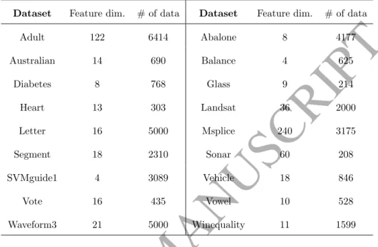
To further compare the proposed method with other OCSVM hyperparame-ter selection methods, we conduct experiments on 18 benchmark datasets down-loaded from the popular UCI Machine Learning Repository1and LIBSVM Data
ACCEPTED MANUSCRIPT
Table 1: Details of Benchmark datasets.
Dataset Feature dim. # of data Dataset Feature dim. # of data
Adult 122 6414 Abalone 8 4177 Australian 14 690 Balance 4 625 Diabetes 8 768 Glass 9 214 Heart 13 303 Landsat 36 2000 Letter 16 5000 Msplice 240 3175 Segment 18 2310 Sonar 60 208 SVMguide1 4 3089 Vehicle 18 846 Vote 16 435 Vowel 10 528 Waveform3 21 5000 Winequality 11 1599
webpage2(the dataset details are summarized in Tab. 1). Since the benchmark
datasets are usually designed for classification, we follow the experimental setup of [21, 17] to test the OCSVM performance with hyperparameters selected by different methods: The values of features are normalized into the interval [−1,1]. For each benchmark dataset, the data from the former half of classes are used as data of target class first, while data from the latter half of classes are viewed as data of outlier class. Data of the target class are randomly partitioned into a training target set and a testing target set. OCSVM is trained using the training target set only, and the testing target set is combined with the data from outlier class as the final testing set for OCC performance evaluation. The random partition is repeated for 10 times to yield the mean OCC performance. Then, the target class and the outlier class are switched and repeat the above procedure to obtain the OCC performance on data from the latter half of classes.
ACCEPTED MANUSCRIPT
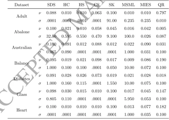
Finally, we average the OCC performance on two halves of classes as the final OCC performance of this benchmark dataset. As to the evaluation metrics, we adopt the widely-used f1-score and Matthews Correlation Coefficient (MCC) [17]. For a rigorous comparison, we perform pairedStudent’s t-testto compare the results yielded by the proposed method and other methods. Ap-value less than 0.05 is considered statistically significant. Those results whose differences from the highest value are not statistically significant are shown in bold for each dataset. The average hyperparemeter values selected by different methods on each dataset in Tab. 2, and the results on benchmark datasets are reported in Tab. 3 (”NaN” in the table means ”Not a number”, which suggests that the trained OCSVM trivially classifies all testing data as outliers).
Table 2: Average hyperparameter values selected on benchmark datasets.
Dataset SDS HC HS CS SK MSML MIES QR Adult ν σ 0.088 .0001 0.010 .0001 0.010 .0001 0.063 .0001 0.100 91.00 0.010 0.235 0.010 0.235 0.797 0.010 Abalone ν σ 0.100 32.50 0.021 0.595 0.010 0.550 0.058 0.470 0.045 9.100 0.016 100.0 0.042 0.026 0.005 0.087 Australian ν σ 0.100 0.065 0.091 0.090 0.012 .0001 0.088 .0001 0.012 .0001 0.022 1.000 0.090 0.031 0.031 0.100 Balance ν σ 0.095 1.000 0.019 0.100 0.021 0.100 0.098 .0001 0.017 0.050 0.009 10.00 0.086 0.072 0.190 0.100 Diabetes ν σ 0.091 1.000 0.028 0.160 0.026 0.115 0.073 .0001 0.019 1.550 0.021 10.00 0.028 0.075 0.018 0.100 Glass ν σ 0.098 0.805 0.030 0.110 0.015 .0001 0.010 .0001 0.100 .0001 0.017 5.950 0.045 0.053 0.147 0.100 Heart ν σ 0.100 .0001 0.010 .0001 0.010 .0001 0.010 .0001 0.100 .0001 0.013 1.000 0.077 0.035 0.182 0.100 Continued on next page
ACCEPTED MANUSCRIPT
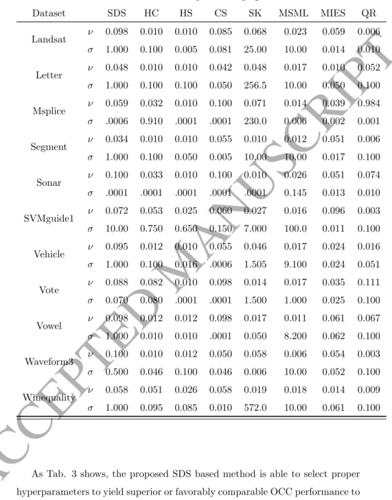
Table 2 – continued from previous page
Dataset SDS HC HS CS SK MSML MIES QR Landsat ν σ 0.098 1.000 0.010 0.100 0.010 0.005 0.085 0.081 0.068 25.00 0.023 10.00 0.059 0.014 0.006 0.010 Letter ν σ 0.048 1.000 0.010 0.100 0.010 0.100 0.042 0.050 0.048 256.5 0.017 10.00 0.010 0.050 0.052 0.100 Msplice ν σ 0.059 .0006 0.032 0.910 0.010 .0001 0.100 .0001 0.071 230.0 0.014 0.006 0.039 0.002 0.984 0.001 Segment ν σ 0.034 1.000 0.010 0.100 0.010 0.050 0.055 0.005 0.010 10.00 0.012 10.00 0.051 0.017 0.006 0.100 Sonar ν σ 0.100 .0001 0.033 .0001 0.010 .0001 0.100 .0001 0.010 .0001 0.026 0.145 0.051 0.013 0.074 0.010 SVMguide1 ν σ 0.072 10.00 0.053 0.750 0.025 0.650 0.060 0.150 0.027 7.000 0.016 100.0 0.096 0.011 0.003 0.100 Vehicle ν σ 0.095 1.000 0.012 0.100 0.010 0.016 0.055 .0006 0.046 1.505 0.017 9.100 0.024 0.024 0.016 0.051 Vote ν σ 0.088 0.070 0.082 0.080 0.010 .0001 0.098 .0001 0.014 1.500 0.017 1.000 0.035 0.025 0.111 0.100 Vowel ν σ 0.098 1.000 0.012 0.010 0.012 0.010 0.098 .0001 0.017 0.050 0.011 8.200 0.061 0.062 0.067 0.100 Waveform3 ν σ 0.100 0.500 0.010 0.046 0.012 0.100 0.050 0.046 0.058 0.006 0.006 10.00 0.054 0.052 0.003 0.100 Winequality ν σ 0.058 1.000 0.051 0.095 0.026 0.085 0.058 0.010 0.019 572.0 0.018 10.00 0.014 0.061 0.009 0.100
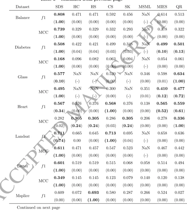
As Tab. 3 shows, the proposed SDS based method is able to select proper hyperparameters to yield superior or favorably comparable OCC performance to other state-of-the-art hyperparameter selection methods on benchmark datasets. Compared with existing pseudo outlier generation based methods (HC, HS and
ACCEPTED MANUSCRIPT
SK), the proposed SDS based method almost constantly outperforms them. In the meantime, it can be seen that hyperparameter selection based on random outliers generated by HC, HS and SK sometimes lead to a trivial solution that simply classifies all testing data into outliers, and their performance is usually poorer than the implicit outlier generation based CS method. As to heuristics based methods, MIES and QR can perform relatively satisfactorily on most datasets, but sometimes their performance can significantly deteriorate since their underlying assumptions on the target data may not hold in such cases. However, MSML yields relatively bad performance and often leads to trivial solution when compared with other methods. To sum up, the proposed method enables OCSVM to achieve fairly good OCC performance on various benchmark datasets, which makes it a promising OCSVM hyperparameter selection method in practical applications.
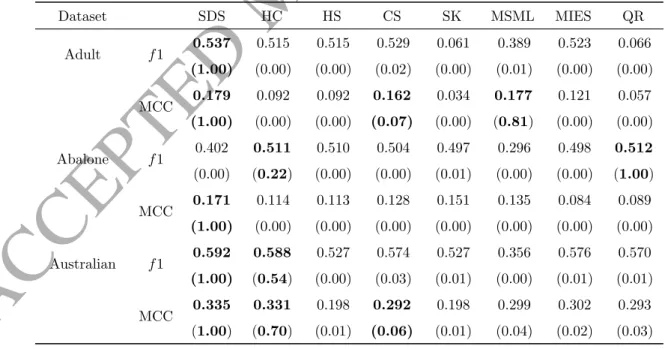
Table 3: Averagef1-score and MCC on benchmark datasets (p-value in the bracket). Boldface
means no statistical difference from the best value (p≥0.05).
Dataset SDS HC HS CS SK MSML MIES QR Adult f1 0.537 (1.00) 0.515 (0.00) 0.515 (0.00) 0.529 (0.02) 0.061 (0.00) 0.389 (0.01) 0.523 (0.00) 0.066 (0.00) MCC 0.179 (1.00) 0.092 (0.00) 0.092 (0.00) 0.162 (0.07) 0.034 (0.00) 0.177 (0.81) 0.121 (0.00) 0.057 (0.00) Abalone f1 0.402 (0.00) 0.511 (0.22) 0.510 (0.00) 0.504 (0.00) 0.497 (0.01) 0.296 (0.00) 0.498 (0.00) 0.512 (1.00) MCC 0.171 (1.00) 0.114 (0.00) 0.113 (0.00) 0.128 (0.00) 0.151 (0.00) 0.135 (0.00) 0.084 (0.00) 0.089 (0.00) Australian f1 0.592 (1.00) 0.588 (0.54) 0.527 (0.00) 0.574 (0.03) 0.527 (0.01) 0.356 (0.00) 0.576 (0.01) 0.570 (0.01) MCC 0.335 (1.00) 0.331 (0.70) 0.198 (0.01) 0.292 (0.06) 0.198 (0.01) 0.299 (0.04) 0.302 (0.02) 0.293 (0.03) Continued on next page
ACCEPTED MANUSCRIPT
Table 3 – continued from previous page
Dataset SDS HC HS CS SK MSML MIES QR Balance f1 0.808 (1.00) 0.471 (0.00) 0.471 (0.00) 0.592 (0.00) 0.456 (0.00) NaN (-) 0.614 (0.00) 0.513 (0.00) MCC 0.739 (1.00) 0.329 (0.00) 0.329 (0.00) 0.332 (0.00) 0.293 (0.00) NaN (-) 0.378 (0.00) 0.322 (0.00) Diabetes f1 0.508 (1.00) 0.422 (0.04) 0.421 (0.04) 0.499 (0.03) 0.348 (0.03) NaN (-) 0.499 (0.10) 0.501 (0.13) MCC 0.168 (1.00) 0.096 (0.00) 0.082 (0.00) 0.062 (0.00) 0.094 (0.00) NaN (-) 0.054 (0.00) 0.061 (0.00) Glass f1 0.577 (0.10) NaN (-) NaN (-) 0.520 (0.00) NaN (-) 0.346 (0.00) 0.598 (0.01) 0.634 (1.00) MCC 0.495 (1.00) NaN (-) NaN (-) 0.300 (0.00) NaN (-) 0.351 (0.01) 0.410 (0.12) 0.477 (0.72) Heart f1 0.567 (0.34) 0.376 (0.00) 0.376 (0.00) 0.568 (1.00) 0.376 (0.00) 0.138 (0.00) 0.565 (0.52) 0.559 (0.61) MCC 0.282 (0.02) 0.305 (0.24) 0.305 (0.24) 0.286 (0.03) 0.305 (0.24) 0.206 (0.00) 0.278 (0.00) 0.336 (1.00) Landsat f1 0.711 (0.74) 0.665 0.00 0.645 (0.00) 0.713 (1.00) 0.695 (0.04) NaN (-) 0.658 (0.00) 0.636 (0.00) MCC 0.611 (1.00) 0.471 (0.00) 0.457 (0.00) 0.547 (0.00) 0.523 (0.00) NaN (-) 0.467 (0.00) 0.442 (0.00) Letter f1 0.601 (1.00) 0.519 (0.00) 0.519 (0.00) 0.515 (0.00) 0.068 (0.00) 0.058 (0.00) 0.514 (0.00) 0.494 (0.00) MCC 0.349 (1.00) 0.145 (0.00) 0.145 (0.00) 0.123 (0.00) 0.079 (0.00) 0.140 (0.00) 0.120 (0.00) 0.138 (0.00) Msplice f1 0.609 (0.00) 0.072 (0.00) 0.693 (1.00) 0.580 (0.00) 0.287 (0.00) 0.266 (0.00) 0.524 (0.00) 0.027 (0.00) Continued on next page
ACCEPTED MANUSCRIPT
Table 3 – continued from previous page
Dataset SDS HC HS CS SK MSML MIES QR MCC 0.385 (1.00) 0.150 (0.00) 0.366 (0.11) 0.381 (0.85) 0.087 (0.00) 0.151 (0.00) 0.371 (0.01) 0.083 (0.00) Segment f1 0.769 (1.00) 0.589 (0.00) 0.588 (0.00) 0.576 (0.00) 0.431 (0.00) 0.436 (0.00) 0.581 (0.00) 0.589 (0.00) MCC 0.644 (1.00) 0.348 (0.00) 0.346 (0.00) 0.309 (0.00) 0.441 (0.00) 0.444 (0.00) 0.325 (0.00) 0.348 (0.00) Sonar f1 0.506 (1.00) 0.422 (0.01) 0.407 (0.00) 0.506 (1.00) 0.407 (0.00) 0.394 (0.00) 0.505 (0.89) 0.498 (0.29) MCC 0.141 (0.00) 0.095 (0.00) 0.067 (0.00) 0.141 (0.00) 0.067 (0.00) 0.232 (1.00) 0.151 (0.00) 0.142 (0.01) SVMguide1 f1 0.838 (1.00) 0.720 (0.00) 0.662 (0.00) 0.727 (0.00) 0.741 (0.01) 0.217 (0.00) 0.755 (0.00) 0.610 (0.00) MCC 0.764 (1.00) 0.568 (0.00) 0.460 (0.00) 0.590 (0.00) 0.634 (0.01) 0.277 (0.00) 0.622 (0.00) 0.345 (0.00) Vehicle f1 0.651 (1.00) 0.564 (0.00) 0.501 (0.00) 0.497 (0.00) 0.442 (0.00) NaN (-) 0.505 (0.00) 0.523 (0.00) MCC 0.542 (1.00) 0.276 (0.00) 0.055 (0.00) 0.032 (0.00) 0.033 (0.00) NaN (-) 0.078 (0.00) 0.129 (0.00) Vote f1 0.733 (1.00) 0.696 (0.21) 0.512 (0.00) 0.690 (0.01) 0.430 (0.00) 0.362 (0.00) 0.678 (0.01) 0.676 (0.17) MCC 0.540 (1.00) 0.523 (0.63) 0.323 (0.01) 0.476 (0.02) 0.281 (0.00) 0.398 (0.00) 0.463 (0.02) 0.536 (0.78) Vowel f1 0.648 (0.24) 0.340 (0.00) 0.340 (0.00) 0.617 (0.00) 0.338 (0.00) 0.169 (0.00) 0.661 (1.00) 0.648 (0.70) MCC 0.552 (1.00) 0.209 (0.00) 0.209 (0.00) 0.380 (0.00) 0.210 (0.00) 0.207 (0.00) 0.460 (0.00) 0.469 (0.04) Continued on next page
ACCEPTED MANUSCRIPT
Table 3 – continued from previous page
Dataset SDS HC HS CS SK MSML MIES QR Waveform3 f1 0.674 (1.00) 0.615 (0.00) 0.632 (0.00) 0.639 (0.00) 0.627 (0.00) NaN (-) 0.637 (0.00) 0.629 (0.00) MCC 0.455 (1.00) 0.269 (0.00) 0.291 (0.00) 0.327 (0.00) 0.329 (0.00) NaN (-) 0.326 (0.00) 0.276 (0.00) Winequality f1 0.519 (1.00) 0.500 (0.00) 0.500 (0.00) 0.497 (0.00) 0.226 (0.00) 0.241 (0.00) 0.501 (0.00) 0.501 (0.00) MCC 0.154 (0.07) 0.053 (0.00) 0.046 (0.00) 0.044 (0.00) 0.182 (1.00) 0.181 (0.88) 0.037 (0.00) 0.039 (0.00)
4.3. Results on MNIST Handwritten Digit Dataset
In addition to the benchmark datasets, we also compare the proposed method with its counterparts on another commonly-used dataset in OCC performance evaluation: MNIST handwritten digit dataset. MNIST dataset provides a la-belled training set with 60000 hand-written digit images (digit 0−9) with a resolution of 28×28 pixels, as well as a separated labelled testing set with 10000 images. For feature extraction, we calculate a 512-D Gist feature [31] to describe each image. For each time, images of one digit from 0−9 in the train-ing set are used as the target class to train one OCSVM. For OCC performance evaluation, the trained OCSVM is used to discriminate this digit from other dig-its (outliers) in the separated testing set. To further validate the effectiveness of the proposed method, we also compare the proposed method with the standard cross-validation (CV) and a ”cheating” method (OPT) by directly using the data from the test set for model validation (the performance of which is there-fore the optimal performance that OCSVM can obtain). In our experiments, SK and MSML perform poorly on MNIST dataset and almost constantly yield trivial solutions (f1 and MCC are both ”NaN”), so we omit the comparison with them in this table. The results are summarized in Tab. 4 below:
ACCEPTED MANUSCRIPT
Table 4: f1-score and MCC on MNIST datasets. Boldface denotes the best results expect
OPT.
Digit SDS HC HS CS MIES QR CV OPT
Digit 0 f1 0.765 0.313 0.313 0.492 0.441 0.309 0.389 0.765 MCC 0.771 0.304 0.304 0.495 0.437 0.305 0.382 0.771 Digit 1 f1 0.938 0.580 0.580 0.836 0.627 0.273 0.720 0.938 MCC 0.933 0.565 0.565 0.820 0.611 0.230 0.694 0.933 Digit 2 f1 0.601 0.344 0.344 0.483 0.360 0.330 0.424 0.601 MCC 0.635 0.331 0.331 0.479 0.349 0.322 0.411 0.635 Digit 3 f1 0.723 0.385 0.385 0.547 0.524 0.403 0.482 0.723 MCC 0.735 0.381 0.381 0.545 0.512 0.408 0.471 0.735 Digit 4 f1 0.564 0.431 0.431 0.564 0.470 0.391 0.519 0.726 MCC 0.558 0.429 0.429 0.558 0.468 0.400 0.507 0.730 Digit 5 f1 0.465 0.341 0.341 0.465 0.375 0.324 0.437 0.677 MCC 0.474 0.348 0.348 0.474 0.385 0.336 0.440 0.699 Digit 6 f1 0.762 0.644 0.644 0.835 0.818 0.646 0.784 0.890 MCC 0.769 0.637 0.637 0.821 0.800 0.645 0.765 0.879 Digit 7 f1 0.757 0.482 0.482 0.573 0.507 0.440 0.552 0.757 MCC 0.747 0.474 0.474 0.562 0.498 0.444 0.532 0.747 Digit 8 f1 0.380 0.296 0.296 0.380 0.373 0.295 0.350 0.719 MCC 0.378 0.280 0.280 0.378 0.365 0.285 0.339 0.731 Digit 9 f1 0.829 0.458 0.458 0.576 0.474 0.236 0.546 0.829 MCC 0.825 0.456 0.456 0.571 0.471 0.191 0.534 0.825
As can be seen in Tab. 4, the proposed SDS based method yields the best OCC performance for 9 out of 10 digits. Specifically, the proposed method evidently outperforms CV method and obtains optimal results for 6 out of 10 digits (digit 0, 1, 2, 3, 7, 9). For other digits that the optimal results are not reached, our method yields the best sub-optimal results among the compared
ACCEPTED MANUSCRIPT
hyperparameter selection methods for 3 digits (digit 4, 5, 8). The implicit outlier generation based method CS obtains equally or slightly worse results than the proposed method. Two classic explicit outlier generation methods HC and HS yield evidently worse OCC performance than the proposed SDS method on each digit. Interestingly, we notice that HC and HS obtain exactly the same results on each digit, which suggest that in fact the random outliers generated by them do not make a difference in a relatively high-dimensional feature space (512-D). When it comes to heuristics based methods, MIES and QR yield comparable or only marginally better OCC performance than random outlier based methods. Consequently, the proposed SDS based method is again proved as an effective method for OCSVM hyperparameter selection.
5. Conclusions
This paper proposes a data shifting based method to automatically select proper hyperparameters of OCSVM, which are vital for OCSVM performance. By self-adaptive negative shifting and positive shifting mechanism, the pro-posed method can efficiently generate high-quality pseudo outlier and target data to estimate the error on outlier class and target class respectively, with-out introducing any new hyperparameters to be tuned by users. It also soundly avoids two major difficulties, determining the number and locations of generated pseudo outlier data, in previous outlier generation based hyperparameter selec-tion methods. Experiments on various synthetic and benchmark datasets verify the effectiveness of the proposed method in comparison with 7 state-of-the-art OCSVM hyperparameter selection methods.
Our future research directions include: (1) Exploring better searching strat-egy like Bayesian Optimization in the hyperparameter space. (2) Since the proposed method can generate new data by self-adaptive data shifting, we will explore its application to imbalanced classification by generating more data for minority classes with insufficient training data.
ACCEPTED MANUSCRIPT
Acknowledgement
This work was sponsored by the National Natural Science Foundation of China (Project no. 61170287, 61232016).
References
[1] D. M. J. Tax, One-class classification, Ph.D. thesis, Delft University of Technology, Netherland (2001).
URLhttp://www.ph.tn.tudelft.hl/~david/thesis.pd
[2] S. Roberts, L. Tarassenko, A probabilistic resource allocating network for novelty detection, Neural Computation 6 (2) (1994) 270–284.
[3] G. Cohen, H. Sax, A. Geissbuhler, Novelty detection using one-class parzen density estimator. an application to surveillance of nosocomial infections., Studies in Health Technology and Informatics 136 (136) (2008) 21–26. [4] N. Japkowicz, C. Myers, M. Gluck, A novelty detection approach to
classi-fication, in: International Joint Conference on Artificial Intelligence, 1995, pp. 518–523.
[5] B. Schlkopf, J. Platt, J. Shawe-Taylor, A. Smola, Estimating the support of a high-dimensional distribution, Neural Computation 13 (7) (2001) 1443. [6] D. M. J. Tax, R. P. W. Duin, Support vector data description, Machine
Learning 54 (1) (2004) 45–66.
[7] Y. Xiao, H. Wang, L. Zhang, W. Xu, Two methods of selecting gaussian kernel parameters for one-class svm and their application to fault detection, Knowledge-Based Systems 59 (2) (2014) 75–84.
[8] D. Xu, E. Ricci, Y. Yan, J. Song, N. Sebe, Learning deep representations of appearance and motion for anomalous event detection, in: British Machine Vision Conference, 2015.
ACCEPTED MANUSCRIPT
[9] V. Mygdalis, A. Iosifidis, A. Tefas, I. Pitas, Graph embedded one-class classifiers for media data classification, Pattern Recognition 60 (C) (2016) 585–595.
[10] R. Perdisci, G. Gu, W. Lee, Using an ensemble of one-class svm classifiers to harden payload-based anomaly detection systems, in: IEEE International Conference on Data Mining, 2006, pp. 488–498.
[11] V. Mygdalis, A. Iosifidis, A. Tefas, I. Pitas, Exploiting subclass information in one-class support vector machine for video summarization, in: IEEE International Conference on Acoustics, Speech and Signal Processing, 2015, pp. 2259–2263.
[12] D. M. J. Tax, R. P. W. Duin, Uniform object generation for optimizing one–class classifiers, Journal of Machine Learning Research 2 (2) (2002) 155–173.
[13] D. M. J. Tax, K. R. Muller, A consistency-based model selection for one-class one-classification, in: International Conference on Pattern Recognition, 2004, pp. 363–366.
[14] W. Fan, M. Miller, S. J. Stolfo, W. Lee, Using artificial anomalies to detect unknown and known network intrusions, in: IEEE International Conference on Data Mining, 2001, pp. 123–130.
[15] H. Deng, R. Xu, Model selection for anomaly detection in wireless ad hoc networks, in: IEEE Symposium on Computational Intelligence and Data Mining, 2007, 2007, pp. 540–546.
[16] A. Nhalmi, A. Kocsor, R. Busa-Fekete, bert, Counter-example generation-based one-class classification, in: European Conference on Machine Learn-ing (ECML), 2007, pp. 543–550.
[17] C. Dsir, S. Bernard, C. Petitjean, L. Heutte, One class random forests, Pattern Recognition 46 (12) (2013) 3490–3506.
ACCEPTED MANUSCRIPT
[18] P. F. Evangelista, M. J. Embrechts, B. K. Szymanski, Some properties of the gaussian kernel for one class learning, in: Artificial Neural Networks -ICANN 2007, International Conference, Porto, Portugal, September 9-13, 2007, Proceedings, 2007, pp. 269–278.
[19] S. Khazai, S. Homayouni, A. Safari, B. Mojaradi, Anomaly detection in hyperspectral images based on an adaptive support vector method, IEEE Geoscience and Remote Sensing Letters 8 (4) (2011) 646–650.
[20] S. Wang, J. Yu, E. Lapira, J. Lee, A modified support vector data descrip-tion based novelty detecdescrip-tion approach for machinery components, Applied Soft Computing 13 (2) (2013) 1193–1205.
[21] Y. Xiao, H. Wang, W. Xu, Parameter selection of gaussian kernel for one-class svm, IEEE Transactions on Cybernetics 45 (5) (2014) 927.
[22] Z. Ghafoori, S. Rajasegarar, S. M. Erfani, S. Karunasekera, C. A. Leckie, Unsupervised parameter estimation for one-class support vector machines, in: Pacific-Asia Conference on Knowledge Discovery and Data Mining, 2016.
[23] Y. Li, L. Maguire, Selecting critical patterns based on local geometrical and statistical information, IEEE Transactions on Pattern Analysis and Machine Intelligence 33 (6) (2011) 1189–1201.
[24] K. Fukunaga, Introduction to statistical pattern recognition (2nd ed.), Aca-demic Press, 1990.
[25] C. Cortes, V. Vapnik, Support-vector networks, Machine Learning 20 (3) (1995) 273–297.
[26] S. Z. Li, J. Lu, Face recognition using the nearest feature line method, IEEE Transactions on Neural Networks 10 (2) (1999) 439–443.
[27] P. Juszczak, D. M. J. Tax, E. Pekalska, R. P. W. Duin, Minimum spanning tree based one-class classifier, Neurocomputing 72 (7-9) (2009) 1859–1869.
ACCEPTED MANUSCRIPT
[28] C. C. Chang, C. J. Lin, Libsvm: A library for support vector machines, Acm Transactions on Intelligent Systems and Technology 2 (3, article 27) (2007) 27.
[29] F. V. D. Heijden, Classification, parameter estimation and state estimation - an engineering approach using matlab, Journal of Time 32 (2) (2011) 194– 194.
[30] D. Tax, Ddtools, the data description toolbox for matlab, version 2.1.2 (June 2015).
[31] A. Oliva, A. Torralba, Modeling the shape of the scene: A holistic repre-sentation of the spatial envelope, International Journal of Computer Vision 42 (3) (2001) 145–175.
ACCEPTED MANUSCRIPT
Siqi Wangis currently a Ph.D. candidate of Computer Science and Technol-ogy in National University of Defense TechnolTechnol-ogy, China. His research interests include pattern recognition and anomaly detection.
Qiang Liu received the Ph.D. degree in computer science and technology from the National University of Defense Technology (NUDT) in 2014. He has contributed several archived journal papers and conference papers, such as IEEE TWC, ICL, NCA, etc. He was invited as a TPC member of Chinacom 2014 and a Session Chair of HPCC 2013. His research interests include protocol design and performance evaluation, machine learning, DoS and other security issues in the emerging wireless networks.
En Zhu received his M.S. degree and Ph.D. degree in Computer Science from the National University of Defense Technology, China, in 2001 and 2005, respectively. He is now working as a full professor in the School of Computer Science, National University of Defense Technology, China. His main research interests include pattern recognition, image processing, and information secu-rity.
Fatih Porikliis an IEEE Fellow and a Professor with the Research School of Engineering, Australian National University, Canberra, ACT, Australia. He is also acting as the Leader of the Computer Vision Group at NICTA, Sydney, NSW, Australia. He received the Ph.D. degree from NYU, New York, NY, USA, in 2002. Previously he served as a Distinguished Research Scientist at Mitsubishi Electric Research Laboratories, Cambridge, MA, USA. He has con-tributed broadly to object detection, motion estimation, tracking, image-based representations, and video analytics. He is the coeditor of two books on Video Analytics for Business Intelligence and Handbook on Background Modeling and Foreground Detection for Video Surveillance. He is an Associate Editor of five journals including IEEE Signal Processing Magazine, SIAM Imaging Sciences, EURASIP Journal of Image & Video Processing, Springer Journal on Machine Vision Applications, and Springer Journal on Real-time Image & Video Pro-cessing. His publications won three best paper awards and he has received the R&D100 Award in the Scientist of the Year category in 2006. He served as the
ACCEPTED MANUSCRIPT
General and Program Chair of several IEEE conferences in the past.
Jianping Yinreceived his M.S. degree and Ph.D. degree in Computer Sci-ence from the National University of Defense Technology, China, in 1986 and 1990, respectively. He is a full professor of computer science in the National University of Defense Technology. His research interests involve artificial intel-ligence, pattern recognition, algorithm design, and information security.