Ranking instances by maximizing the area under ROC curve

Ranking Instances by Maximizing

the Area under ROC Curve

H. Altay Gu¨venir,

Member,

IEEE, and Murat Kurtcephe

Abstract—In recent years, the problem of learning a real-valued function that induces a ranking over an instance space has gained importance in machine learning literature. Here, we propose a supervised algorithm that learns a ranking function, called ranking instances by maximizing the area under the ROC curve (RIMARC). Since the area under the ROC curve (AUC) is a widely accepted performance measure for evaluating the quality of ranking, the algorithm aims to maximize the AUC value directly. For a single categorical feature, we show the necessary and sufficient condition that any ranking function must satisfy to achieve the maximum AUC. We also sketch a method to discretize a continuous feature in a way to reach the maximum AUC as well. RIMARC uses a heuristic to extend this maximization to all features of a data set. The ranking function learned by the RIMARC algorithm is in a human-readable form; therefore, it provides valuable information to domain experts for decision making. Performance of RIMARC is evaluated on many real-life data sets by using different state-of-the-art algorithms. Evaluations of the AUC metric show that RIMARC achieves significantly better performance compared to other similar methods.

Index Terms—Ranking, data mining, machine learning, decision support

Ç

1

I

NTRODUCTION

I

Nthis paper, we propose a binary classification metho-dology that ranks instances based upon how likely they are to have a positive label. Our method is based on receiver operating characteristic (ROC) analysis, and attempts to maximize the area under the ROC curve (AUC); hence, the algorithm is called ranking instances by maximizing the area under ROC curve (RIMARC). The RIMARC algorithm learns a ranking function which is a linear combination of nonlinear score functions constructed for each feature separately. Each of these nonlinear score functions aims to maximize the AUC by considering only the corresponding feature in ranking. All continuous features are first discretized into categorical ones in a way that optimizes the AUC. Given a single categorical feature, it is possible to derive a scoring function that achieves the maximum AUC. We show the necessary and sufficient condition that such a scoring function for a single feature has to satisfy for achieving the maximum AUC. Computing the score function for a categorical feature requires only one pass over the training data set. Missing feature values are simply ignored. The AUC value, obtained on the training data, for a single feature, reflects the effect of that feature in the correct ranking. Using these AUC values as weights, the RIMARC algorithm combines these score functions, learned for each feature, into a single ranking function.

The main characteristics of the RIMARC algorithm can be summarized as follows: It achieves comparably high AUC values. Its time complexity for both learning and applying the ranking function is relatively low. Being a nonparametric method, it does not require tuning of parameters to achieve the best performance. It is robust to missing feature values. Finally, the ranking function learned is in a human readable form that can be easily interpreted by domain experts, listing the effects (weight) of features and how their particular values affect the ranking. The RIMARC algorithm is simple and easy to implement. In cases where a data set is collected from experiments for research purposes, the researchers may be more interested in the effects of the features and their particular values on ranking than the particular ranking function.

In the next section, the ranking problem is revisited. Section 3 covers ROC, AUC and research on AUC maximization. In Section 4, the RIMARC method and implementation details are given. Section 5 presents the empirical evaluation of RIMARC on real-world data sets. Section 6 discusses the related work. Finally, Section 7 concludes with some suggestions for future work.

2

R

ANKING

The ranking problem can be viewed as a binary classification problem with additional ordinal information. In the binary classification problem, the learner is given a finite sequence of labeled training examples z¼ ððx1; y1Þ;. . .;ðxn; ynÞÞ, where the xi are instances in some instance space X and the yi are labels in Y ¼ fp;ng, and the goal is to learn a binary-valued function h:X!Y that predicts accurately labels of future instances.

The problem of finding a function that ranks positive instances higher than the negative ones is referred as the bipartiteranking problem. Here, a training data setD, from

. The authors are with the Department of Computer Engineering, Bilkent University, Ankara 06800, Turkey.

E-mail: guvenir@cs.bilkent.edu.tr, kurtcephe@gmail.com.

Manuscript received 26 Feb. 2012; revised 15 Oct. 2012; accepted 17 Oct. 2012; published online 23 Oct. 2012.

Recommended for acceptance by B.C. Ooi.

For information on obtaining reprints of this article, please send e-mail to: tkde@computer.org, and reference IEEECS Log Number TKDE-2012-02-0128. Digital Object Identifier no. 10.1109/TKDE.2012.214.

an instance space X, is given, where the instances come from a set of two categories, positive and negative, represented as {p,n}. UsingD, the goal is to learn a ranking function r:X!IR that ranks future positive instances higher than negative ones. In other words, the functionris expected to assign higher values to positive instances than to negative ones. Then, the instances can be ordered using the values provided by the ranking function.

3

I

NTRODUCTION TO

ROC A

NALYSIS

The ROC graph is a tool that can be used to visualize, organize, and select classifiers based on their performance [22]. It has become a popular performance measure in the machine learning community after it was realized that accuracy is often a poor metric to evaluate classifier performance [33], [41], [42].

The literature on ROC is more established to deal with binary classification problems than multiclass ones. At the end of the classification phase, some classifiers simply map each instance to a class label (discrete output). Some other classifiers, such as naı¨ve Bayes or neural networks are able to estimate the probability of an instance belonging to a specific class (continuous valued output).

Binary classifiers produce a discrete output represented by only one point in the ROC space, since only one confusion matrix is produced from their classification output. Continuous-output-producing classifiers can have more than one confusion matrix by applying different thresholds to predict class membership. All instances with a score greater than the threshold are predicted to bepclass and all others are predicted to benclass. Therefore, for each threshold value, a separate confusion matrix is obtained. The number of confusion matrices is equal to the number of ROC points on an ROC graph. With the method proposed by Domingos [15], it is possible to obtain ROC curves even for algorithms that are unable to produce scores.

Let a set of instances, labeled as por n, be ranked by some scoring function. Given a threshold value, instances whose score is below are predicted asn, and those with score higher thanare predicted asp. For a given threshold value,TP is equal to the number of positive instances that have been classified correctly andFPis equal to the number of negative instances that have been misclassified.

The ROC graph can be plotted as the fraction of true positives out of the positives (TPR = true positive rate) versus the fraction of false positives out of the negatives (FPR= false positive rate). The values ofTPRandFPRare calculated by using (1). In this equation,Nis the number of total negative instances and P is the number of total positive instances

T P R¼T P

P ; F P R¼ F P

N : ð1Þ

For each possible distinct value, a distinct (FPR,TPR) value is computed. The ROC space is a 2D space with a range of [0, 1] on both axes. In ROC space the vertical axis represents the true positive rate of a classification output, while the horizontal axis represents the false positive rate. That is, each (FPR,TPR) pair corresponds to a point on the ROC space. In a data set with s distinct classifier scores,

there aresþ1ROC points, including the trivial (0, 0) and (1, 1) points.

Although ROC graphs are useful for visualizing the performance of a classifier, a scalar value is needed to compare classifiers. Bradley [5] proposes the area under the ROC curve as a performance measure.

The ROC graph space is a one-unit square. The highest possible AUC value is 1.0, which represents the perfect ordering. In ROC graphs, a 0.5 AUC value means random guessing has occurred and values below 0.5 are not realistic as they can be negated by changing the decision criteria of the classifier.

The AUC value of a classifier is equal to the probability that the classifier will rank a randomly chosen positive instance higher than a randomly chosen negative instance [22].

In an empirical ROC curve, the AUC is usually estimated by the trapezoidal rule. According to this rule, trapezoids are formed using the observed points as corners, the areas of these trapezoids are computed and then they are added up. Fawcett [22] proposed efficient algorithms for generat-ing the ROC points and computgenerat-ing the AUC.

It can be shown that the area under the ROC curve is closely related to the Mann-Whitney U, which tests whether positives are ranked higher than negatives. AUC is also equivalent to the Wilcoxon test of ranks [30].

4

RIMARC

RIMARC is a simple, yet powerful, ranking algorithm designed to maximize the AUC metric directly. The RIMARC algorithm reduces the problem of finding a ranking function for the whole set of features into finding a ranking function for a single categorical feature, and then combines these functions to form one covering all features. We will show that it is possible to determine a ranking function that achieves the maximum possible AUC for a single categorical feature. During the training phase, the RIMARC algorithm first discretizes the continuous features by a method called MAD2C, proposed by Kurtcephe and Guvenir [35]. The MAD2C method discretizes a continuous feature in such a way that results in a set of categorical values so that the AUC of the new categorical feature is the maximum. At this point, all the features are categorical. Then, the score for a valuevof a featurefis assigned to be the probability of a training instance that has the valuevfor the feature f to have the class label p. During the computation of the score values, instances whose value for the feature f is missing are simply ignored. For each feature, the values are sorted in the increasing order of their score, and the AUC is computed. Finally, the weight of a feature f is computed as, wf ¼2ðAUCðfÞ 0:5Þ where AUC(f) is the AUC obtained on the featuref. That is, the weight of a feature is a linear function of its AUC value calculated using the training instances whose value for that feature is known. A higher value of AUC for a feature is an indication of its higher relevance in determining the class label. For example, if the AUC computed for a featurefis 1, than it means that all instances in the training set can be ranked by using only the values off. Hence, we can expect that new query instances can also be ranked correctly by

using f only. The training method of the RIMARC algorithm is given in Algorithm 2.

For a given query, q, the ranking function, r(), of the RIMARC algorithm returns a real valuerðqÞin the range of [0, 1]. This value r(q) is roughly the probability that the instanceqhas the class labelp. It is only a rough estimate of the probability, since it is very likely that no other instance with exactly the same feature values has been observed in the training set. The ranking function of the RIMARC algorithm determines this estimated probability by comput-ing the weighted average of probabilities computed on single features, as shown in Algorithm 1.

Algorithm 1.The ranking function.

Algorithm 2.Training in RIMARC.

In the following sections, we will show how the ranking function and the score values can be defined for a single categorical feature.

4.1 Single Categorical Feature Case

A categorical feature has a finite set of choices as its values. Let V ¼ fv1;. . .vkg be a the set of categorical values for a given feature. In that case, the training data setDis a set of instances represented by a vector of feature value and class label as <vi; c>, where vi2V and c2 fp;ng. A ranking functionr:V ! [0, 1] can be defined to rank the values in V. According to this ranking function, a valuevjcomes after a valueviif and only ifrðviÞ< rðvjÞ; hence,rdefines a total

ordering on the setV, that isvivj. A pair of consecutive values vi and viþ1 defines an ROC point Ri on the ROC space. The coordinates of the point Ri are (F P Ri; T P Ri). The instances of D can then be ranked according to the values ofrðvi) corresponding to their feature values,vi.

Let D be a data set with a single categorical feature whose value set is V ¼ fv1;. . .; vkg, and r:V ! [0, 1] be the ranking function that orders the values ofV, such that viviþ1ifrðviÞ< rðviþ1Þ, for all values of 1ik. Since there is only one feature, this function r(), ranks the instances, directly.

It is interesting to note that, if the values of the ranking function for two consecutive values vi and viþ1 are swapped, then the only change in the ROC curve is that the ROC point corresponding to the vi and viþ1 values moves to a new location so that the slopes of the line segments adjacent to that ROC point are swapped.

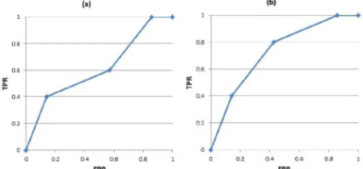
For example, consider a data set with a single categorical feature, given as D ¼ fða;nÞ;ðb;pÞ;ðb;nÞ;ðb;nÞ;ðb;nÞ;

ðc;pÞ;ðc;pÞ;ðc;nÞ;ðc;nÞ;ðd;pÞ;ðd;pÞ;ðd;nÞg, w h e r e V ¼ fa;b;c;dg. If a ranking function r orders the values of V as acbd, with rðaÞ< rðcÞ< rðbÞ< rðdÞ, the ROC curve shown in Fig. 1a will be obtained. If the ranking function is modified so that values of rðbÞ and rðcÞ are swapped, the ROC curve shown in Fig. 1b will be obtained. A similar technique was used earlier by earlier by Flach and Wu [24] to create better prediction models for classifiers.

This property of the ROC spaces helps to remove the concavities in an ROC curve, resulting in a larger AUC. To obtain the maximum AUC value, the ROC curve has to be convex. Hence, we will show how to construct the ranking function so that the resulting ROC curve is guaranteed to be convex.

Note that the slope of the line segment between two consecutive ROC pointsRi andRiþ1is

si ¼T P RiT P Riþ1

F P RiF P Riþ1: ð2Þ In order for the ROC curve to be convex, the slopes of all line segments connecting consecutive ROC points starting from the trivial ROC point (1, 1) must be nondecreasing, as shown in Fig. 2. Therefore, the condition for a convex ROC curve is

8i

1i<k si siþ1: ð3Þ

Fig. 1. Effect of swapping the values of the ranking function of two feature values.

Using (2), 8i 1i<k T P Riþ1T P Riþ2 F P Riþ1F P Riþ2 T P RiT P Riþ1 F P RiF P Riþ1: By definition,T P Ri¼T Pi

P , whereT Piis the number of true positives with valuevi. Further, due to the ordering of values, T Pi ¼PiþT Piþ1, where Pi is the number of p-labeled instances with valuevi. Hence,

T P RiT P Riþ1¼T P Ri P T P Riþ1 P ¼ 1 P PiþT Piþ1T Piþ1¼Pi P: Similarly, F P RiF P Riþ1¼Ni N: T P Riþ1T P Riþ2¼Piþ1 P and

F P Riþ1F P Riþ2¼Niþ1

N :

Therefore, the condition in (3) can be rewritten as

8i 1i<k Piþ1=P Niþ1=N Pi=P Ni=N: Finally, 8i 1i<k Piþ1 Niþ1 Pi Ni: ð4Þ

That is, to obtain a convex ROC curve, the condition in (4) must be satisfied for all ROC points. In other words, to achieve the maximum AUC, the ranking function has to satisfy the following condition:

8i

1i<krðviþ1Þ> rðviÞiff Piþ1 Niþ1

Pi

Ni: ð5Þ

Further, any ranking function that satisfies (5) will result in the same ROC curve and achieve the maximum AUC. For example, the ranking function defined asrðviÞ ¼NPii will result in a convex ROC curve.

It is also important to note that, given a data set with a single categorical feature, there exists exactly one convex ROC curve, and it corresponds to the best ranking.

The general assumptions for ranking problems are given below: 8i 1ikPi 0; 1ik8i Ni 0; P¼X k 1 Pi>0; N ¼X k 1 Ni>0:

Although the data set is guaranteed to have at least one instance with class labelpand one instance with labeln, it is possible that for some values ofi,Ni may be 0. In such cases the ranking function defined as rðviÞ ¼Pi=Ni will have an undefined value. To avoid such problems, the RIMARC algorithm defines the ranking function as

rðviÞ ¼ Pi

PiþNi: ð6Þ

Note that, since8i1ikPiþNi>0,r(vi) is defined for all values ofi. To see that the ranking function defined in (6) satisfies the condition in (5), note that if

8i 0i<n Piþ1 Piþ1þNiþ1 Pi PiþNi; then 8i

0i<n Piþ1ðPi þNiÞ PiðPiþ1 þNiþ1Þ; and 8i 0i<n Piþ1 Niþ1 Pi Ni:

The ranking function given in (6) has another added benefit, in that it is simply the probability of the p label among all instances with valuevi. Such a probability value is easily interpretable by humans.

However, note that the commonly used Laplace esti-mate, defined as Piþ1

PiþNiþ2 does not satisfy the condition in (5).

4.1.1 The Effect of the Choice of the Class Labeling on the AUC

To calculate theP andN values, one of the classes should be labeled aspand the other class asn, but one can question the effect this choice has on the AUC value. It is possible to show that the AUC value of a categorical feature is independent from the choice of class labels by using the value from the Wilcoxon-Mann-Whitney statistics.

In (7), the AUC formula based on the Wilcoxon-Mann-Whitney statistics is given. The set Dp represents the

p-labeled instances andDnrepresents then-labeled instances. Dpiis the ranking of theith instance in theDpset, similarly, Dnj, is the ranking of theith instance in theDpset

AUC¼ PP i¼1 PN j¼1fðDpi; DnjÞ P N ; f¼ 1 if Dpi> Dnj 0 if Dpi< Dnj 0:5 if Dpi¼Dnj 2 6 4 3 7 5: ð7Þ

The dividend part of the AUC formula in (7) counts the number ofp-labeled instances for each element of theDpset whose ranking is higher than any element of the Dn set. Then, AUC is calculated by dividing this summation by the multiplication of thep-labeled andn-labeled elements.

It is straightforward that the divisor part of the AUC formula is independent of the choice of the class labels.

Fig. 2. Relation between the slopes of two consecutive line segments in a convex ROC curve.

Assume that the ranking function given in (6) is used on the data setD, and Dp and Dn sets are formed. Letni be the number ofn-labeled instances whose ranking is lower than theith element of theDpset and letri be the score assigned to this element. When the classes are swapped, the new ranking score r0_i is equal to1ri. Using this property, all instance scores are subtracted from 1. However, this operation simply reverses the ranking of the instances. So the formula in (7), which calculates the value of AUC, using the ranking of the instances, is independent of the choice of class labeling.

4.1.2 An Example Toy Data Set

Consider a toy training data set with a single categorical feature given in Table 1. To calculate the AUC value of this particular feature, assume that the ranking scores are calculated by the function in (6). The ranking scores of the categorical values are as follows: rðaÞ ¼0:25; rðbÞ ¼ 0:33; rðcÞ ¼0:67, and rðdÞ ¼1. The version of the data set sorted by the ranking function is given in Table 2. In this example, the value of P is 7 and the value ofN is 6. The AUC value of this feature is calculated by using (7), as 34:5

76¼0:82. When the class labels are swapped (nlabels are replaced byplabels and vice versa) the ranking scores are also swapped. The sorted version of the swapped toy data set is given in Table 3. Since the relative ranking of the instances does not change, the AUC value of the new ranking is also is 0.82.

4.2 Handling Continuous Features

Having determined the requirement for a ranking function for a categorical feature to achieve the maximum possible AUC, the next problem is to develop a mechanism for handling the continuous features. An obvious and trivial ranking function maps each real value seen in the training set with the class labelpto 1 and each real value with the class label n to 0. This risk function will result in the maximum possible value for AUC, which is 1.0. However, such a risk function will over fit the training data, and will be undefined for unseen values of the feature, which are very likely to be seen in a query instance. The first requirement for a risk function for a continuous feature is that it must be defined for all possible values of that continuous feature. A straightforward solution to this requirement is to discretize the continuous feature by grouping all consecutive values with the same class value

to a single categorical value. The cut off points can be set to the middle point between feature values of differing class labels. The ranking function, then, can be defined using the function given in (6) for categorical features. Although this would result in a ranking function that is defined for all values of a continuous function, it would still suffer from the over fitting problem. To overcome this problem, the RIMARC algorithm makes the following assumption.

Assumption.For a continuous feature, either the higher values are indicators of thepclass and lower values are indicators of the of thenclass, or vice versa.

Although there exist some features in real-world domains that do not satisfy this assumption, in the data sets we examined this assumption is satisfied in general.

This assumption is also consistent with the interpreta-tions of the values of continuous features in many real-world applications. For example, in a medical domain, a high value of fasting blood glucose is an indication for diabetes. On the other hand, low fasting blood glucose is an indication of another health problem, called hypoglycemia.

4.2.1 The MAD2C Method

As explained above, the RIMARC algorithm requires all features to be categorical. Therefore, the continuous features in a data set need to be converted into categorical ones, through discretization. The aim of a discretization method is to find the proper cut-points to categorize a given continuous feature.

The MAD algorithm given in [35] is defined for multiclass data sets. It is designed to maximize the AUC value by checking the ranking quality of values of a continuous feature. A special version of the MAD algorithm, called MAD2C, defined for two-class problems, is used in RIMARC. The MAD2C algorithm first sorts the training instances in ascending order. Sorting is essential for all discretization methods to produce intervals that are as homogenous as possible. After the sorting operation, feature values are used as hypothetical ranking score values and the ROC graph of the ranking on that feature is constructed. The AUC of the ROC curve indicates the overall ranking quality of the continuous feature. To obtain the maximum AUC value, only the points on the convex hull must be selected. The minimum number of points that form the convex hull is found by eliminating the points that cause concavities on the ROC graph. In each pass, the MAD2C method compares the slopes in the order of the creation of the hypothetical lines, finds the junction points (cut-points) that cause concavities and eliminates them. This process is repeated until there is no concavity remaining on the graph. The points left on the graph are the cut-points, which will be used to discretize the feature.

TABLE 1

Toy Training Data Set with One Categorical Feature

TABLE 2

Toy Training Data Set with Score Values

The ranking scores of the instances are calculated and they are sorted in ascending order.

TABLE 3

Training Data Set with Class Labels Swapped

The ranking scores are recalculated and instances are sorted in ascending order.

It has been proven that the MAD2C method finds the cut-points that will yield the maximum AUC. It is also shown that the cut-points found by MAD2C never separate two consecutive instances of the same class. This is an important property, expected from a discretization method. The MAD2C method is preferred among other discretiza-tion methods since it has been shown in empirical evaluations that MAD2C has lower running time in two-class data sets and helps the two-classification algorithms to achieve a higher performance than other well-known discretization methods on AUC basis [35].

4.2.2 A Toy Data Set Discretization Example

To visualize the discretization process using the MAD2C method, a toy data set is given in Table 4. After the sorting operation, the ROC points are formed. The ROC graph for the example in Table 4 is given in Fig. 3. In this example, the higher F1 values are indicators of thepclass. If the lower values of feature F1 were indicators of thepclass, then thep

and nclass labels would be swapped and the ROC graph below the diagonal would have been obtained. Note that these two ROC graphs are symmetric about the diagonal.

The first pass of the MAD2C algorithm is shown in Fig. 4. All points below or on the diagonal are ignored since they have no positive effect on the maximization of AUC. Then the points causing concavities are eliminated. MAD2C converged to the convex hull in one pass for this example, as shown in Fig. 4. The set of points left on the graph are reported as the discretization cut-points.

4.3 The RIMARC Algorithm

The training phase of the RIMARC algorithm is given in Algorithm. 1. In the training phase, first, using the MAD2C algorithm, all continuous features are discretized and

converted into categorical features. Ranking scores are calculated for each value of a given categorical feature, including discretized continuous features. In this step, the ranking function defined in (6) is used to obtain the optimal ranking for the features. Then, the training instances are sorted according to their ranking values computed in the previous step. Since the ranking function used by RIMARC always results in a convex ROC curve, the AUC is always equal to or greater than 0.5.

The AUC of a feature indicates its relevance in the ranking of an instance. For example, if a feature has 1 as its AUC, than the ranking score of a new instance can be computed by considering only that feature. On the other hand, a feature with 0.5 as its AUC should be ignored. Therefore, the RIMARC algorithm uses a function of AUC to determine the weight of a feature in ranking. Since it is easier for human experts to interpret the weight values in the range of 0 to 1, the RIMARC algorithm uses a weightwf for a featuref computed as

wf¼2ðAUCf0:5Þ: ð8Þ The ROC curve of an irrelevant feature is simply a diagonal line from (0, 0) to (1, 1), withAUC¼0:5. The weight function in (8) assigns 0 to such irrelevant features to ignore them in computing the ranking function. The score values and weights of the features are stored for the querying phase. The model learned for the single function for the toy data set in Table 4 is shown in Fig. 5. The model contains the weight of the feature and a nonlinear ranking function.

The testing phase of the RIMARC method is straightfor-ward, as shown in Algorithm 2. For each feature, the ranking score corresponding to the value of the feature in

TABLE 4

A Toy Data Set for Visualizing MAD2C

Fig. 3. Visualization of the ROC points in two-class discretization.

Fig. 4. Final cut-points after the first pass of convex hull algorithm.

the query instance is used. The ranking score of this feature is weighted by its weight computed in the training phase. The computation of the ranking function for a query instanceqis given in (9). rðqÞ ¼ P fwf: PrðpjqfÞ P fwf ; wf¼ 2ðAUCf0:5Þ; qfis known; 0; qfis missing: ð9Þ

The maximization of AUC for the whole feature set is a challenging problem. Cohen et al. [11] showed that the problem of finding the ordering that agrees best with a learned preference function is NP-Complete. As a solution, this weighting mechanism is used as a simple heuristic to extend this maximization over the whole feature set.

In (9),PrðpjqfÞis the probability that the query instance qbeingp-labeled, given that the value of featurefinqisqf and wf is the weight of the feature f, computed by (8). Finally, to obtain the weighted average, the sum of all weighted score values is divided by the sum of the weights of all used (known) features. That is, rðqÞ is the weighted probability of the instanceq has the labelp.

4.4 Time Complexity

The training time complexity of the MAD2C algorithm is Oðn2_{Þ, in the worst case and OðnlognÞ in the best case,} where n is the number of training instances. Since the distribution of the data is not known, calculation of the average-case is not possible theoretically. However, in empirical evaluations, the MAD2C method converged to the convex hull in very close to linear time [35] excluding sorting time. After discretizing the numerical features, the time complexity of the RIMARC algorithm is OðmvlogvþnÞ, wherem is the number of features and v is the average number of categorical values per feature. That is, the training time complexity of the RIMARC is bounded by that of the MAD2C algorithm. The time complexity of the querying step is simplyO(m).

4.5 Interpretation of the Predictive Model of RIMARC

The RIMARC method not only provides the ranking score as a single real value for a given query instance, but also reports the model used for ranking, which can provide useful information to domain experts. For example, a high feature weight value indicates that the corresponding feature is a highly effective factor in the given domain. On the other hand, domain experts may choose to ignore features with low weights, potentially reducing the cost of record keeping.

Some of the categorical features are formed by dis-cretizing continuous features. Assume that the effect of age is investigated on a real-world domain, such as medicine. Although such a feature can be discretized into child, youth, adult, and elderly, by some experts, the intervals should be chosen carefully since they can affect the ranking performance of the system. Further, in some experimental domains this kind of prior knowledge may not even be available. The MAD2C method used in RIMARC learns the proper intervals to maximize the AUC during the training phase.

5

E

MPIRICAL

E

VALUATIONS

To support the theoretical background of the RIMARC algorithm with empirical results, it is compared with 27 different machine learning algorithms on AUC basis. To experiment with real-life domains, we selected some of the two-class data sets from the UCI machine learning repository [25]. We chose 10 data sets with two class labels. The properties of the data sets are given in Table 5.

To perform the comparisons, 27 different classification algorithms are selected from the WEKA package [28]. Since the AUC values are used for the measure of the predictive performance, only the classification methods that provide prediction probability estimates are employed in experi-mental results. However, the SVM algorithms do not provide these probabilities directly. Therefore, the LibSVM library is used for the SVM algorithm [9], since it provides probability estimates using the second approach proposed by Wu et al. [50]. To compare RIMARC with ranking algorithms that try to maximize the AUC directly, the SVM-Perf is also chosen, since the source code is available from the author [34].

Although RIMARC is a nonparametric method, it would be unfair not to optimize the parametric classifiers used in the evaluation. Therefore, the parameters of the SVM-based classifiers (SVM-RBF and SVM-Perf-RBF), naı¨ve Bayes and J48 (decision tree) algorithms are optimized. For all other classifiers, their default settings in the WEKA package are used.

5.1 Predictive Performance

Researchers have reported that some of the algorithms that aim to maximize AUC directly do not obtain significantly better AUC values than the ones designed to maximize accuracy [13], [29]. Therefore, it is important to show that RIMARC can outperform accuracy-maximizing algorithms statistically significantly, as well the ranking algorithms based on classifiers.

Stratified tenfold cross validation is used to calculate AUC values for each data set. As shown in Table 6, the RIMARC method outperformed all algorithms on the average AUC metric. Further, Wilcoxon signed-rank test is used to determine whether the differences in averages are significant [48]. This statistical method is chosen, since it is a nonparametric method and does not assume normal distribution as pairedt-test does. According to the Wilcoxon

TABLE 5

Real Life Data Sets for Evaluation

signed-rank test on a 95 percent confidence level (the same level will be used for other statistical tests), RIMARC statistically significantly outperforms 17 of the 27 machine learning algorithms. These algorithms include naı¨ve Bayes, decision trees (PART, C4.5) and SVM with an RBF kernel and SVM-Perf with an RBF kernel. The RIMARC algorithm outperformed the other 10 algorithms, as well, but the differences between the averages for these algorithms are not statistically significant.

One important point should be mentioned about the SVM algorithms. As seen in Table 6, SVM has the worst predictive performance among all the classification algo-rithms because of the absence of parameter tuning. There-fore, we optimized the SVM-RBF and SVM-Perf-RBF by using an inner cross validation to find the optimum gamma value for the RBF kernel. The optimized versions of SVM are called SVM-RBF-Opt and SVM-Perf-RBF-Opt. Gamma value ranged from 0.01 up to 0.1 in 10 steps. As seen in Table 6, optimization boosted the performance of SVM-RBF significantly (0.701 versus 0.887). However, SVM-Perf-RBF did not gain such a significant improvement by optimiza-tion (0.754 versus 0.763). As a result, it can be claimed that the nonparametric RIMARC algorithm outperforms SVM-based methods significantly, even when they are optimized on the gamma value.

Entropy-MDLP discretization method by Fayyad and Irani [19] is used on the naı¨ve Bayes method to improve predictive performance. Since Dougherty et al. [16] showed that using discretization improves naı¨ve Bayes predictive performance, an improvement was expected.

However, as Table 6 shows, the discretization did not improve the performance of naı¨ve Bayes at all. The C parameter is optimized by using inner cross validation for J48 algorithm (decision tree). The C-value is ranged from 0.1 up to 0.5 in 10 steps.

The classifier with the highest AUC after RIMARC was the Adaboost method. As an ensembling algorithm, Adaboost uses a base classifier, which is DecisionStump by default in the WEKA package.

The classification algorithms such as Logistic (multi-nomial logistic regression model) and ClassViaReg (classi-fication via regression) achieve high AUC values. As mentioned above, these models are highly used in the domain of medicine, and in this work their predictive performance is validated.

Another point that deserves mentioning is that the average standard deviation among the individual AUC values of the RIMARC algorithm is the smallest among all the algorithms we tested.

Similar to the naı¨ve Bayes classifier, the RIMARC algorithm assumes that the features are independent of each other. Holte [32] has pointed out that most of the data sets in the UCI repository are such that, for classification, their attributes can be considered independently of each other, which explains the success of the RIMARC algorithm on these data sets. Similar observation is also made by Gu¨venir and S¸irin [27].

5.2 Running Time

The RIMARC method is designed to be simple, effective, and fast. It computes the scores for each value for a categorical

TABLE 6

Predictive Performance Comparison

The comparison of the predictive performance of RIMARC algorithm with other algorithms on the AUC metric. Ten data sets are used during evaluation. Standard deviation values are given in parenthesis. Algorithms marked with ++ are outperformed by RIMARC on average, with a statistically significant difference. Algorithms marked with + are outperformed by RIMARC on average, with no statistically significant difference (higher is better).

feature in close to linear time. MAD2C requires more time since it uses sorting. Although the time complexity of the RIMARC algorithm is shown to be low, empirical experi-ments were conducted to support this claim.

The overall running times of the training phase of 25 different algorithms on the data sets are compared with that of RIMARC. The training times of all algorithms are measured using Java Virtual Machine’s CPU time and 100 results are averaged.

Since the outsourced libraries were used for the SVM-RBF and SVM-Perf-SVM-RBF algorithms, they are not included in the running time experiments. The results of the overall running time for the other algorithms are shown in Table 7. The RIMARC algorithm, on the basis of running times, significantly outperformed 13 of the algorithms according to the Wilcoxon signed-rank test [49]. These methods outperformed by RIMARC are indicated by the ++ symbol in Table 7. Seven algorithms significantly outperformed RIMARC. These algorithms are shown with a symbol. The differences between the other five methods in the table and RIMARC are not significant. Note that all of the algorithms that significantly outperformed the RIMARC algorithm in terms of the running time are outperformed by RIMARC in terms of the AUC metric.

6

R

ELATED

W

ORK

The problem of learning a real-valued function that induces a ranking or ordering over an instance space has gained importance in machine learning literature. Information retrieval, credit-risk screening or estimation of risks

associated with a surgery are some examples of the application domains. In this paper, we consider the ranking problem with binary classification data. It is known as the bipartite ranking problem, which refers to the problem of learning a ranking function from a training set of examples with binary labels [2], [10], [26]. Agarwal and Roth [2] studied the learnability of bipartite ranking functions and showed that learning linear ranking functions over Boolean domains is NP-hard. In the bipartite ranking problem, given a training set of instances with labels either positive or negative, one wants to learn a real-valued ranking function that can be used for an unseen case to associate a measure of being close to positive (or negative) class. For example, in a medical domain, a surgeon may be concerned with estimating the risk of a patient who is planned to undergo a serious operation. A successful ranking (or scoring) function is expected to return a high value if the operation carries high risks for that patient. Specific ranking functions have been developed for particular domains, such as information retrieval [18], [47], finance [6], medicine [12], [14], [44], fraud detection [20], and insurance [17]. Some of these methods are dependent on statistical models while some are based on machine learning algorithms. A binary classification algorithm that returns a confidence factor associated with the class label can be used for bipartite ranking, where the confidence factor associated with a positive label (or the complement associated with a negative label) can be taken as the value of the ranking function.

The area under the receiver operating characteristic curve (AUC) is a widely accepted performance measure for evaluating the quality of a ranking function [5], [22]. It has been shown that the AUC represents the probability that a randomly chosen positive instance is correctly assigned a higher rank value than a randomly selected negative instance. Further, this probability of correct ranking is equal to the value estimated by the nonpara-metric Wilcoxon statistic [30]. Also, AUC has important features such as insensitivity to class distribution and cost distributions [5], [22], [33]. Agarwal et al. [1] showed what kind of classification algorithms can be used for ranking problems and proved theorems about generalization prop-erties of AUC.

Some approximation methods aiming at maximizing the global AUC value directly have been proposed by researchers [31], [39], [51]. For example, Ataman et al. [3] proposed a ranking algorithm by maximizing AUC with linear programming. Brefeld and Scheffer [7] presented an AUC maximizing support vector machine. Rakotomamonjy [43] proposed a quadratic programming-based algorithm for AUC maximization and showed that under certain conditions 2-norm soft margin support vector machines can also maximize AUC. Toh et al. [46] designed an algorithm to optimize the ROC performance directly according to the fusion classifier. Ferri et al. [23] proposed a method to locally optimize AUC in decision tree learning, and Cortes and Mohri [13] proposed boosted decision stumps. To maximize AUC in rule learning, several algorithms have been proposed [4], [21], [40]. A nonparametric linear classifier based on the local max-imization of AUC was presented by Marrocco et al. [38]. A ROC-based genetic learning algorithm has been proposed by Sebag et al. [44]. Marrocco et al. [37] used linear

TABLE 7

Running Time Performance Comparison

The comparison of the average running time performance of RIMARC with other algorithms (in ms). Ten data sets are used during evaluation. Algorithms marked with ++ are outperformed by RIMARC on running time basis with a statistically significant difference. Algorithms marked with -- outperformed RIMARC on running time basis with a statistically significant difference. Algorithms marked with + are outperformed by RIMARC on average, and the ones marked with - outperform RIMARC on average, but with no significant difference. (Lower is better).

combinations of dichotomizers for the same purpose. Freund et al. [26] gave a boosting algorithm combining multiple rankings. Cortes and Mohri [13] showed that this approach also aims to maximize AUC. A method by Tax et al. [45] that weighs features linearly by optimizing AUC has been applied to the detection of interstitial lung disease. Ataman et al. [3] advocated an AUC-maximizing algorithm with linear programming. Joachims [34] pro-posed a binary classification algorithm by using SVM that can maximize AUC. Ling and Zhang [36] compared AUC-based tree-augmented naı¨ve Bayes (TAN) and error-AUC-based TAN algorithms; the AUC-based algorithms are shown to produce more accurate rankings. More recently, Calders and Jaroszewicz [8] suggested a polynomial approximation of AUC to optimize it efficiently. Linear combinations of classifiers are also used to maximize AUC in biometric scores fusion [46]. Han and Zhao [29] proposed a linear classifier based on active learning that maximizes AUC.

7

C

ONCLUSIONS AND

F

UTURE

W

ORK

In this paper, we presented a supervised algorithm for learning a ranking function, called RIMARC.

We have shown that for a categorical feature, there is only one ordering that gives the maximum AUC. Then, we showed the necessary and sufficient condition that a ranking function for a single categorical feature has to satisfy to achieve this ordering. As a result, we proposed a ranking function that achieves the maximum possible AUC value on a single categorical feature. This ranking function is based on the probability ofpclass for each value of that feature. The MAD2C algorithm used by RIMARC discre-tizes continuous features in a way that yields the maximum AUC, as well. The RIMARC algorithm used AUC values of features as their weights in computing the ranking function. With this simple heuristic, we computed the weighted average of all feature value scores to achieve maximum AUC over the whole feature set. Since the RIMARC algorithm uses all available feature values and ignores the missing ones, it is robust to missing feature values.

We presented the characteristics of the ranking function learned by the RIMARC algorithms and how it can be interpreted. The ranking function is in a human readable form that can be easily interpreted by domain experts. The feature weights learned help the experts to determine how they affect the ranking.

We compared RIMARC with 27 different algorithms. According to our empirical evaluations, RIMARC signifi-cantly outperformed 17 algorithms on an AUC basis and 13 algorithms on a time basis. It also outperformed all algorithms on the average AUC and 16 of them on an average running time basis.

It is also worth noting that the RIMARC algorithm is a non-parametric machine learning algorithm. As such, it does not have any parameters that need to be tuned to achieve high performance on a given data set; hence, it can be used by domain experts who are not experienced in tuning machine learning algorithms.

To improve the performance of RIMARC, instead of using the weighted average, other approaches can be investigated. Another possible direction for future work would be to experiment with methods that ensemble RIMARC with other ranking algorithms.

R

EFERENCES

[1] S. Agarwal, T. Graepel, R. Herbrich, S. Har-Peled, and D. Roth, “Generalization Bounds for the Area under the ROC Curve,”

J. Machine Learning Research,vol. 6, pp. 393-425, 2005.

[2] S. Agarwal and D. Roth, “Learnability of Bipartite Ranking Functions,”Proc. 18th Ann. Conf. Learning Theory,2005.

[3] K. Ataman, W.N. Street, and Y. Zhang, “Learning to Rank by Maximizing AUC with Linear Programming,” Proc. IEEE Int’l Joint Conf. Neural Networks (IJCNN),pp. 123-129, 2006.

[4] H. Bostro¨m, “Maximizing the Area under the ROC Curve Using Incremental Reduced Error Pruning,” Proc. Int’l Conf. Machine Learning Workshop (ICML ’05),2005.

[5] A.P. Bradley, “The Use of the Area under the ROC Curve in the Evaluation of Machine Learning Algorithms,”Pattern Recognition,

vol. 30, no. 7, pp. 1145-1159, 1997.

[6] B.O. Bradley and M.S. Taqqu, “Handbook of Heavy-Tailed Distributions in Finance,” Financial Risk and Heavy Tails,

S.T. Rachev, ed., pp. 35-103, Elsevier, 2003.

[7] U. Brefeld and T. Scheffer, “AUC Maximizing Support Vector Learning,”Proc. ICML Workshop ROC Analysis in Machine Learning,

2005.

[8] T. Calders and S. Jaroszewicz, ”Efficient AUC Optimization for Classification,” Proc. 11th European Conf. Principles and Practice of Knowledge Discovery in Databases (PKDD ’07),pp. 42-53, 2007.

[9] C.C. Chang and C.C. Lin, “LIBSVM: A Library for Support Vector Machines,” http://www.csie.ntu.edu.tw/~cjlin/libsvm, 2001.

[10] S. Cleme´nc¸on, G. Lugosi, and N. Vayatis, “Ranking and Scoring Using Empirical Risk Minimization,” Proc. 18th Ann. Conf. Learning Theory (COLT ’05),pp. 1-15, 2005.

[11] W.W. Cohen, R.E. Schapire, and Y. Singer, “Learning to Order Things,”J. Artificial Intelligence Research,vol. 10, pp. 243-270, 1998.

[12] R.M. Conroy, K. Pyo¨ra¨la¨, and A.P. Fitzgerald, “Estimation of Ten-Year Risk of Fatal Cardiovascular Disease in Europe: The SCORE Project,”European Heart J.,vol. 11, pp. 987-1003, 2003.

[13] C. Cortes and M. Mohri, “AUC Optimization versus Error Rate Minimization,”Proc. Conf. Neural Information Processing Systems (NIPS ’03),vol. 16, pp. 313-320, 2003.

[14] R.B. D’Agostino, S.V. Ramachandran, and J. Pencina, “General Cardiovascular Risk Profile for Use in Primary Care: The Framingham Heart Study,”Circulation,vol. 17, pp. 743-753, 2008.

[15] P. Domingos, “MetaCost: A General Method for Making Classifiers Cost-Sensitive,” Proc. Fifth ACM SIGKDD Int’l Conf. Knowledge Discovery and Data Mining,pp. 155-164, 1999.

[16] J. Dougherty, R. Kohavi, and M. Sahami, “Supervised and Unsupervised Discretization of Continuous Features,”Proc. 12th Int’l Conf. Machine Learning,pp. 194-202, 1995.

[17] K. Dowd and D. Blake, “After VaR: The Theory, Estimation, and Insurance Applications of Quantile-Based Risk Measures,” The J. Risk and Insurance,vol. 73, no. 2, pp. 193-229, 2006.

[18] W. Fan, M.D. Gordon, and P. Pathak, “Discovery of Context-Specific Ranking Functions for Effective Information Retrieval Using Genetic Programming,” IEEE Trans. Knowledge and Data Eng.,vol. 16, no. 4, pp. 523-27, Apr. 2004.

[19] U. Fayyad and K. Irani, “On the Handling of Continuous-Valued Attributes in Decision Tree Generation,”Machine Learning,vol. 8, pp. 87-102, 1992.

[20] T. Fawcett and F. Provost, “Adaptive Fraud Detection,” Data Mining and Knowledge Discovery,vol. 1, pp. 291-316, 1997.

[21] T. Fawcett, “Using Rule Sets to Maximize ROC Performance,”

Proc. IEEE Int’l Conf. Data Mining (ICDM ’01),pp. 131-138, 2001.

[22] T. Fawcett, “An Introduction to ROC Analysis,”Pattern Recogni-tion Letters,vol. 27, pp. 861-874, 2006.

[23] C. Ferri, P. Flach, and J. Hernandez, “Learning Decision Trees Using the Area under the ROC Curve,” Proc. 19th Int’l Conf. Machine Learning (ICML ’02),pp. 139-146, 2002.

[24] P. Flach and S. Wu, “Repairing Concavities in ROC Curves,”Proc. UK Workshop Computational Intelligence,pp. 38-44, 2003.

[25] A. Frank and A. Asuncion, “UCI Machine Learning Repository,” School of Information and Computer Science, Univ. of California, http://archive.ics.uci.edu/ml, 2010.

[26] Y. Freund, R. Iyer, R.E. Schapire, and Y. Singer, “An Efficient Boosting Algorithm for Combining Preferences,” J. Machine Learning Research,vol. 4, pp. 933-969, 2003.

[27] H.A. Gu¨venir and_I. S¸irin, “Classification by Feature Partitioning,”

[28] M. Hall, E. Frank, G. Holmes, B. Pfahringer, P. Reutemann, and I.H. Witten, “The WEKA Data Mining Software: An Update,”

SIGKDD Explorations,vol. 11, no. 1, pp. 10-18, 2009.

[29] G. Han and C. Zhao, “AUC Maximization Linear Classifier Based on Active Learning and Its Application,”Neurocomputing,vol. 73, nos. 7-9, pp. 1272-1280, 2010.

[30] J.A. Hanley and B.J. McNeil, “The Meaning and use of the Area under a Receiver Operating Characteristic (ROC) Curve,” Radi-ology,vol. 143, pp. 29-36, 1982.

[31] A. Herschtal and B. Raskutti, “Optimising the Area under the ROC Curve Using Gradient Descent,” Proc. Int’l Conf. Machine Learning,pp. 49-56, 2004.

[32] R.C. Holte, “Very Simple Classification Rules Perform Well on Most Commonly Used Data Sets,” Machine Learning, vol. 11, pp. 63-91, 1993.

[33] J. Huang and C.X. Ling, “Using AUC and Accuracy in Evaluating Learning Algorithms,” IEEE Trans. Knowledge and Data Eng.,

vol. 17, no. 3, pp. 299-310, Mar. 2005.

[34] T. Joachims, “A Support Vector Method for Multivariate Performance Measures, “Proc. Int’l Conf. Machine Learning (ICML),

2005.

[35] M. Kurtcephe and H.A. Gu¨venir, “A Discretization Method Based on Maximizing the Area under ROC Curve,” Int’l J. Pattern Recognition and Artificial Intelligence,vol. 27, no. 1, article 1350002, 2013.

[36] C.L. Ling and H. Zhang, “Toward Bayesian Classifiers with Accurate Probabilities,”Proc. Sixth Pacific-Asia Conf. Advances in Knowledge Discovery and Data Mining,pp. 123-134, 2002.

[37] C. Marrocco, M. Molinara, and F. Tortorella, “Exploiting AUC for Optimal Linear Combinations of Dichotomizers,”Pattern Recogni-tion Letters,vol. 27, no. 8, pp. 900-907, 2006.

[38] C. Marrocco, R.P.W. Duin, and F. Tortorella, “Maximizing the Area under the ROC Curve by Pairwise Feature Combination,”

Pattern Recognition,vol. 41, pp. 1961-1974, 2008.

[39] M.C. Mozer, R. Dodier, M.D. Colagrosso, C. Guerra-Salcedo, and R. Wolniewicz, “Prodding the ROC Curve: Constrained Optimi-zation of Classifier Performance,”Proc. Conf. Advances in Neural Information Processing Systems,vol. 14, pp. 1409-1415, 2002.

[40] R. Prati and P. Flach, “Roccer: A ROC Convex Hull Rule Learning Algorithm,” Proc. ECML/PKDD Workshop Advances in Inductive Rule Learning,pp. 144-153, 2004.

[41] F. Provost and T. Fawcett, “Analysis and Visualization of Classifier Performance: Comparison under Imprecise Class and Cost Distributions,”Proc. Third Int’l Conf. Knowledge Discovery and Data Mining,pp. 43-48, 1997.

[42] F. Provost, T. Fawcett, and R. Kohavi, “The Case against Accuracy Estimation for Comparing Induction Algorithms,”Proc. 15th Int’l Conf. Machine Learning,pp. 445-453, 1998.

[43] A. Rakotomamonjy, “Optimizing Area under ROC Curve with SVMS,” Proc. Workshop ROC Analysis in Artificial Intelligence,

pp. 71-80, 2004.

[44] M. Sebag, J. Aze, and N. Lucas, “ROC-Based Evolutionary Learning: Application to Medical Data Mining,”Artificial Evolu-tion,vol. 2936, pp. 384-396, 2004.

[45] D.J.M. Tax, R.P.W. Duin, and Y. Arzhaeva, “Linear Model Combining by Optimizing the Area under the ROC Curve,”Proc. IEEE 18th Int’l Conf. Pattern Recognition,pp. 119-122, 2006.

[46] K.A. Toh, J. Kim, and S. Lee, “Maximizing Area under ROC Curve for Biometric Scores Fusion,”Pattern Recognition,vol. 41, pp. 3373-3392, 2008.

[47] F. Wang and X. Chang, “Cost-Sensitive Support Vector Ranking for Information Retrieval,”J. Convergence Information Technology,

vol. 5, no. 10, pp. 109-116, 2010.

[48] M. Wasikowski and X. Chen, “Combating the Small Sample Class Imbalance Problem Using Feature Selection,”IEEE Trans. Knowl-edge Discovery and Data Eng.,vol. 22, no. 10, pp. 1388-1400, Oct. 2010.

[49] F. Wilcoxon, “Individual Comparisons by Ranking Methods,”

Biometrics,vol. 1, pp. 80-83, 1945.

[50] T.-F. Wu, C.-J. Lin, and W.C. Wen, “Probability Estimates for Multi-Class Classification by Pairwise Coupling,” J. Machine Learning Research,vol. 5, pp. 975-1005, 2004.

[51] L. Yan, R. Dodier, M.C. Mozer, and R. Wolniewicz, “Optimizing Classifier Performance via the Wilcoxon-Mann-Whitney Statis-tics,”Proc. 20th Int’l Conf. Machine Learning,pp. 848-855, 2003.

H. Altay Gu¨ venir received the BS and MS degrees in electronics and communications engineering from Istanbul Technical University, in 1979 and 1981, respectively, and the PhD degree in computer engineering and science from Case Western Reserve University in 1987. He joined the Department of Computer Engi-neering at Bilkent University in 1987. He has been a professor and serving as the chairman of the Department of Computer Engineering since 2001. His research interests include artificial intelligence, machine learning, data mining, and intelligent data analysis. He is a member of the IEEE and the ACM.

Murat Kurtcephereceived the first MSc degree in computer science from Bilkent University, Ankara, Turkey, where he worked on machine learning and data mining, especially on dis-cretization and risk estimation methods with Prof. H. Altay Gu¨venir. He received the second MSc degree from the Computer Science De-partment at Case Western University, where he worked with Professor Meral Ozsoyoglu on query visualization and pedigree data querying. Currently, he is working at NorthPoint Solutions, New York, focusing on regulatory compliance reporting applications.

. For more information on this or any other computing topic, please visit our Digital Library atwww.computer.org/publications/dlib.