Lecture Notes 7
Exchange Rate Overshooting
International Economics: Finance Professor: Alan G. Isaac
7 Exchange Rate Overshooting 1
7.1 Overshooting: Core Considerations . . . 3
7.1.1 Covered Interest Parity with Regressive Expectations . . . 4
7.1.2 Liquidity Effects and Overshooting . . . 8
7.1.3 The Algebra of Overshooting . . . 10
7.2 Implied Real Changes . . . 12
7.2.1 CIPRE : Real Version . . . 12
7.2.2 Liquidity Effects and Non-Neutrality of Money . . . 15
7.3 The Long Run In Sticky-Price Models . . . 17
7.3.1 The Real Interest Differential Model . . . 19
7.4 Money Market Considerations . . . 23
7.4.1 Overshooting with Sticky Prices . . . 25
7.5 Simple Empirical Considerations . . . 30
7.5.2 Forward Rates . . . 31
7.5.3 VAR Analysis . . . 32
7.6 Conclusion . . . 33
Terms and Concepts . . . 34
Problems for Review . . . 34
7.7 Dornbusch (1976) . . . 35
7.7.1 Regressive Expectations . . . 35
7.7.2 Rational Expectations . . . 37
7.7.3 Unanticipated Policy Shocks . . . 41
7.7.4 Anticipated Shocks . . . 43
In chapter 3, our development of the monetary approach to flexible exchange rates relied on two key ingredients: the Classical model of price determination, and an exogenous real exchange rate. We found that the monetary approach had some notable early empirical successes. But we also found that as data accumulated under the new flexible exchange rate regimes, the simple monetary approach appeared increasingly unsatisfactory. The present chapter considers whether the problem lies in attempting to use the monetary approach model, which has a long-run orientation, to describe short-run exchange-rate movements.
The widespread adoption of floating exchange rates in the early 1970s brought unexpected volatility of the nominal exchange rate. The large movements of the nominal exchange rate, coupled with the relative inertia of the price level, produced large fluctuations in the real exchange rate (and therefore large deviations from purchasing power parity). The monetary approach model of chapter 3 treats such real exchange rate movements as exogenous, but it is clearly desirable to explain them.
Increasing the scope of our models seldom comes without costs, and our attempt to endogenize the real exchange rate is no exception. The most popular models of short-run real-exchange-rate movements abandon the simplifying Classical assumption of perfectly flexible prices. These models treat the price level as “sticky” in the short run. This chapter develops such a “sticky-price” exchange-rate model. We find we must therefore abandon two key simplifying assumptions of the monetary approach model: the exogeneity of the real interest rate, and the exogeneity of the real exchange rate. Our sticky-price model will predict large short-run deviations from purchasing power parity, such as those described in chapter 5.
In sticky-price models, monetary policy influences real interest rates and the real exchange rate. When prices are “sticky”, any change in the nominal money stock becomes a change in the real money stock, which will generally imply a change in the interest-rate. Similarly, short-run nominal-exchange-rate fluctuations will imply corresponding real exchange rate fluctuations. There is an immediate benefit for our exchange rate models: we are no longer
7.1. OVERSHOOTING: CORE CONSIDERATIONS 3
forced to treat persistent deviations from purchasing power parity, such as those we discussed in chapter 5, as purely exogenous. Instead our explanation short-run nominal-exchange-rate movements becomes an explanation of short-run real-exchange-rate movements. Sticky-price models also offer new insights into the sources of exchange-rate volatility. In particular, they offer an explanation of why exchange rates may be much more volatile than monetary policy.
7.1
Overshooting: Core Considerations
Suppose an economy is disturbed by an unanticipated exogenous change, which we call a
shock. This might be a change in monetary or fiscal policy, but it need not be policy related. We say the endogenous variable exhibits overshooting in response to this shock if its short-run movement exceeds the change in its steady-state value.
For example, given the long-run neutrality of money, a one-time, permanent increase in the money supply will eventually lead to a proportional depreciation of the steady-state value of the currency. If the short-run depreciation is more than proportional, then the short-run depreciation of the spot rate is greater than the depreciation of its steady-state value. We say such an economy exhibits exchange-rate overshooting in response to money-supply shocks.
Popular models of such exchange rate overshooting have three key ingredients: covered interest parity, regressive expectations, and a liquidity effect of money supply changes. You are already familiar with the covered interest parity relationship: it is just the requirement that domestic assets bear the same rate of return as fully hedged foreign assets. This means that i = i∗ +fd. If we decompose the forward discount on the domestic currency into expected depreciation and a “risk premium,” then we can write this asi=i∗+ ∆se+rp.
Once again we see that we must deal with exchange-rate expectations if we wish to discuss the determination of exchange rates. Instead of the rational-expectations assumption, this chapter will adopt the slightly more general regressive-expectations assumption. Expectations are “regressive” when the exchange rate is expected to move toward its
long-run value. This is intended to capture the common-sense idea that if you think that the exchange rate is currently overvalued, then you also expect it to depreciate toward its long-run value.
The final key ingredient is that monetary policy has a liquidity effect in the short run. This means, for example, that expansionary monetary policy lowers the real interest rate in the short run. These three ingredients—covered interest parity, regressive expectations, and short-run liquidity effects—can be combined to illustrate why the exchange rate may overshoot in response to monetary policy changes.
7.1.1
Covered Interest Parity with Regressive Expectations
The first ingredient in our exchange-rate overshooting models is covered interest parity. In chapter 2 we saw that covered interest parity is implied by perfect capital mobility in the assets markets. Recall that covered interest parity is just the requirement of equivalent returns on equivalent assets. This is the first core ingredient of overshooting models.
i−i∗−rp = ∆se (7.1)
Hereiis the domestic nominal interest rate, i∗ is the foreign interest rate,rp is the expected excess return on the domestic asset, and ∆se is the expected rate of depreciation of the
spot exchange rate. Note the presence of the expected rate of depreciation. As with the simple monetary approach model, this makes consideration of exchange rate expectations unavoidable. Holding all else constant, covered interest parity implies that the domestic interest rate must be higher when expected depreciation is higher. This implied positive correlation between interest rates and expected depreciation is summarized in figure 7.1.
The second ingredient in our exchange-rate overshooting models isregressive expectations. Expectations formation is called “regressive” when a variable is expected to close any gap between its current level and its long-run equilibrium level. So if exchange-rate expectations
7.1. OVERSHOOTING: CORE CONSIDERATIONS 5 ∆se i 0 i∗+rp CIP
Figure 7.1: Covered Interest Parity
are regressive, a spot rate that is above its long-run equilibrium level is expected to fall towards that level. The expected rate of real depreciation depends on the gap between the current exchange rate and its long-run equilibrium level.1
∆se =−Θ(S/S¯) (7.2)
Here ¯Sis the “full-equilibrium value” of the spot rate, which we will discuss more below. The function Θ determines the expected speed of adjustment of the real exchange rate toward its long-run equilibrium value, based on the current gap between the spot rate and its full-equilibrium value. When S is relatively high, it is expected to fall; when it is relatively low, it is expected to rise. That, in a nutshell, is the regressive expectations hypothesis. The implied negative correlation between the current spot rate and the expected rate of depreciation is illustrated in figure 7.2.
While regressive expectations are in many ways a plausible description of expectations
1A popular formulation of this relationship sets expected rate of depreciation to a proportion of the percentage gap between the spot rate and its long-run equilibrium level. Let δs represent the percentage deviation ofs from its long-run value. We can then write the regressive expectations hypothesis as ∆se=
−Θ(δs). In terms ofS, this becomes
∆se=−Θ S ¯ S −1
In an inflationary environment, expected depreciation is naturally given a slightly different formulation. See section 7.1.3.
¯ S ∆se S H H H H H H H H H H H H H RE|S¯ 0
Figure 7.2: Regressive Expectations
formation, many economists will be bothered by any abandonment of the assumption of rational expectations. At the theoretical level, it is therefore reassuring that in many over-shooting models, rational expectations proves to be a special case of regressive expectations. In this case, regressive expectations are not only easier to model but actually encompass the behavior implied under rational expectations.
Given the central role played by regressive expectations in the model of overshooting, it is nevertheless natural to inquire as to the realism of this assumption. There are survey studies that offer some support for this the regressive expectations hypothesis. Frankel and Froot (1987) estimate expected speed of adjustment as 0.2 using such data, which offers a reasonable matche to regression estimates of the speed of adjustment.
We saw that covered interest parity implies that the interest rate will be lower when the exchange rate is expected to appreciate. We also saw that regressive expectations imply that the exchange rate is expected to appreciate when it is high (i.e., when it is above its long-run equilibrium rate). Together these imply that the interest rate will be lower when the exchange rate is higher. That is, together (7.1) and (7.2) imply (7.3).
i−i∗−rp =−Θ(S/S¯) (7.3)
7.1. OVERSHOOTING: CORE CONSIDERATIONS 7
economy.) For now, we also treat the risk premium as exogenous.2 Then for any given
long-run equilibrium spot rate, equation (7.3) implies a negative relationship between the interest rate and the spot rate, which is represented by the CIPRE curve in figure 7.3.
We draw a CIPRE curve for agiven long-run equilibrium spot rate. For example, consider the CIPRE curve associated with ¯S1 in figure 7.3. We can deduce from the figure that the
interest rate compatible with zero expected depreciation is i0. You can see this because the
figure indicates that when the interest rate isi0, the spot rate equals its long-run equilibrium level (from which it is not expected to move). When the interest rate is lower, say at isr, the spot rate must be higher. How high? It must be high enough that expected movement of the exchange rate, as implied by regressive expectations, offsets the interest rate differential, as required by covered interest parity.
¯ S1 s ¯ S2 Ssr s s i S H H H H H H H H H H H H H H H H H H H H H H H H H H CIPRE|S1¯ CIPRE|S2¯ i0 isr
Figure 7.3: Exchange Rate Overshooting
Now consider the effect of a change in the long-run equilibrium spot rate. In figure 7.3, the shift up of the CIPRE curve represents the effects of an increase in the long-run equilibrium spot rate from ¯S1 to ¯S2. The interest rate i0 is compatible with covered interest
parity only when expected depreciation is zero, but expected depreciation is zero only when the spot rate equals the long-run equilibrium exchange rate. Therefore the CIPRE curve shifts up by exactly the change in the long-run equilibrium exchange rate. If this takes place without a change in the interest rate, as in the monetary approach to flexible rates, then
Figure 7.4: Interest-Rate Differential Versus Exchange Rate (UK vs US)
Source: http://www.ny.frb.org/newsevents/news/markets/2013/fxq313.pdf, Chart 6.
no overshooting is involved. However, in the presence of liquidity effects, this relationship between spot rates and interest rates provides a basis for exchange rate overshooting.
7.1.2
Liquidity Effects and Overshooting
The third ingredient in our exchange-rate overshooting models is the liquidity effects of monetary policy. In the Classical model, a one-time, permanent, unanticipated increase in the money supply has no effect on the interest rate. The interest rate is simply the fixed real rate plus expected inflation, and a one-time change in the money supply has no effect on expected inflation. A one-time, permanent increase in the growth rate of the money supply, on the other hand, has an effect on the interest rate. Expected inflation rises, and there is a corresponding rise in the interest rate. Again, the real interest rate remains unchanged. One way of describing these outcomes is to say that in the Classical model, monetary policy has no liquidity effects.
7.1. OVERSHOOTING: CORE CONSIDERATIONS 9
When prices are sticky, interest rates are likely to change when the money supply changes. For example, a one-time, permanent, unanticipated increase in the money supply will increase the real money supply (since prices do not move proportionally). If the interest rate falls in response, we say there is a liquidity effect. This can cause overshooting of the exchange rate. To see this, reconsider equation (7.3). Holding all other variables constant, a fall in the interest rate implies that S/S¯ must rise. The increase in the spot rate must exceed the increase in the long-run equilibrium exchange rate. There is exchange rate overshooting.
These considerations are captured in figure 7.3. The lower CIPRE curve represents covered interest parity under regressive expectations, given the initial steady-state spot rate
¯
S1. Begin at the initial steady state at (i0,S¯1). We then introduce a one-time, permanent,
unanticipated change in the money supply. A one-time, permanent money supply increase should have no effect on the steady-state interest rate, but the steady-state spot rate should depreciate. We represent this as the increase from ¯S1 to ¯S2. The upper CIPRE curve represents covered interest parity under regressive expectations, given the new steady-state spot rate ¯S2. The short-run liquidy effect is represented by the fall in the interest rate from i0 toisr. As a result, we find that in the short run, the exchange rate depreciates from ¯S1 to Ssr, overshooting the new steady-state spot rate.
This overshooting result turned on three elements: convered interest parity, regressive expectations, and a liquidity effect. If a one-time, permanent increase in the money supply has a liquidity effect, there is a fall in the interest rate. With high capital mobility, we might expect this lower interest rate to initiate massive capital outflows and thereby an exchange rate depreciation. However the interest parity condition can be satisfied if the lower interest rate is offset by an expected appreciation of the domestic currency. With regressive expectations, appreciation is expected only when the spot rate is above its steady-state value. Thus the spot rate does depreciate, but only until it is enough above the steady-state spot rate that expected appreciation offsets the interest differential. That is, the money supply increase causes a short-run depreciation of the spot rate that exceeds the
depreciation of its steady-state value. There is exchange rate overshooting.
7.1.3
The Algebra of Overshooting
The algebra will again be a matter of covered interest parity, regressive expectations, and a characterization of liquidity effects. Recall that the covered interest parity condition can be stated as in (7.1), which is restated; here for convenience.
i−i∗−rp = ∆se (7.1)
We will once again conjoin covered interest parity and regressive expectations, but before doing so we will slightly modify the regressive expectations hypothesis.
In an inflationary environment, expected depreciation of the nominal exchange rate is not naturally given the regressive formulation of equation (7.2). Letting ¯s be the long-run (steady-state) value of s, we reformulate the regressive expectations hypothesis in the following natural way.3
∆set = ∆¯set −θ(st−¯st) (7.4)
3In natural units, we could write this as
%∆Se= %∆ ¯Se−θS− ¯ S ¯ S
One way to look at this begins with regressive expectations for thereal exchange rate. ∆qe=−θ δq
To move from our regressive expectations formulation for expected real exchange-rate depreciation to a characterization of expected nominal echange rate depreciation, first note that
∆se= ∆qe+ ∆pe−∆p∗e
We can reasonably expect inflation even when the price level is at its “full equilibrium” level ¯p: the full equilibrium level can change over time (for example, as the money stock grows). We account for this by allowing inflation expectations to incorporate a “core-inflation” rate.
∆pe=−θ δp+ ∆¯pe ∆p∗e=−θ δp∗+ ∆¯p∗e
ex-7.1. OVERSHOOTING: CORE CONSIDERATIONS 11
Again, θ is the speed at which the exchange rate is expected to move toward its long-run level, and ∆¯se is the rate at which the full-equilibrium exchange rate is expected to change
over time.4 ∆¯se is the rate at which the equilibrium spot exchange rate is expected to
change, and it is a natural addition to expected depreciation. For example, suppose the spot rate were at its current equilibrium value. It would still be expected to depreciate if the domestic country is a high inflation country, since such depreciation is required for the spot rate to remain at its equilibrium value over time. This implies that individuals take inflation differentials into account in forming their expectations about spot rate depreciation, and as we saw in the previous chapter, they are justified in doing so. In an inflationary environment, it is natural to allow expectations to include the underlying core-inflation differential.
Together, covered interest parity and regressive expectations imply (7.5).
i−i∗−rp = ∆¯se−θ(s−s¯) (7.5)
Solving (7.5) for s yields (7.6).
s= ¯s− 1
θ(i−i
∗−
∆¯se−rp) (7.6)
Equation (7.6) has been the subject of a great deal of empircal scrutiny, which is discussed in section 7.3.1. First, however, we show that (7.6) implies overshooting by considering the
pected nominal exchage-rate depreciation as
∆se=−θ δq−θ δp+ ∆¯pe =−θ δs+ ∆¯pe−∆¯p∗e As long as the is no long-run trend inq, this can be rewritten as
∆se=−θ δs+ ∆¯se
4A simpler formulation, lacking the term ∆¯se, of regressive expectations is often applied illustratively.
See the formulation in section 7.1.1, which is essentially the illustrative treatment offered in, for example, Dornbusch (1976)) and Florentis et al. (1994). However, empirical work must allow for the long-run inflation observed in real economies. As a result, the equilibrium spot rate must be characterized as changing over time.
effect of a one-time, permanent increase in the money supply. ds dh = ds¯ dh − 1 θ di dh > ds¯ dh (7.7)
In the presence of liquidity effects, the increase in the money supply will immediately reduce the interest rate, so thatdi/dh <0. We also expect that a permanent increase in the money supply will depreciate the long-run spot rate, so that ds/dh >¯ 0. So the spot rate moves move than the long-run equilibrium exchange rate. That is, the exchange rate overshoots in response to a one-time, permanent increase in the money supply.
7.2
Implied Real Changes
7.2.1
CIPRE : Real Version
We can give an equivalent formulation in terms of real interest rates and the expected depreciation of the real exchange rate.
(i−∆pe)−(i∗−∆p∗e)−rp = (∆p∗e−∆pe+ ∆se) (7.8)
r−r∗ −rp = ∆qe (7.9)
Holding all else constant, note that covered interest parity implies that the domestic real interest rate is higher when expected real depreciation is higher. This implied positive correlation between real interest rates and real expected depreciation is summarized in figure 7.1.
If real and nominal exchange rates were variable after the generalized float, so were inflation and real interest rates. Still, in the 1970s, real interest rate variation was low enough that real interest rates were often treated as constants. In addition, if we rank the developed countries by their inflation rates in the 1970s and by their nominal interest rates,
7.2. IMPLIED REAL CHANGES 13 ∆qe r 0 r∗+rp CIP
Figure 7.5: Covered Interest Parity: Real Version
the rankings are roughly the same. For example, Switzerland had the lowest inflation and nominal interest rates, while Britain had higher inflation and higher nominal interest rates. When inflation rates surged with the oil price shocks of 1973 and 1979, interest rates sharply increased as well.
But the 1980s saw a pattern of responses to tight monetary policy that shattered the relationships of the 1970s. Even though inflation rates began declining in 1981, nominal interest rates remained high. Real interest rates were high and varied among nations. For example, U.S. real interest rates were particularly high, while U.S. inflation fell more rapidly than the inflation of its major trading partners. The pattern of large and variable real interest differentials continued into the 1990s, when German real interest rates rose above the moderating U.S. rates.
Consider 1984, when U.S. ex post real interest rates were high. The high rates of return were possibly simply a surprise, or perhaps they were due to a large change in expected excess returns (rp). The remaining possibility interests us most: the real interest differential may have reflected expected real appreciation, as in figure 7.1. In this case, the high ex post
real interest rates were anticipated and reflected an expectation of a real depreciation of the dollar.
¯ Q ∆q∗ Q H H H H H H H H H H H H H RE 0
Figure 7.6: Regressive Expectations: Real Exchange Rate
lower when a real exchange rate appreciation is expected. We also saw that, under regressive expectations, the real exchange rate will be expected to appreciate when it is high (i.e., above its long-run equilibrium rate). Together these imply that the real interest rate will be lower when the real exchange rate is higher. That is, together (7.9) and (3) imply (7.10).
r−r∗−rp =−θ δq (7.10)
For now, treat the foreign real interest rate as an exogenous constant (as in a small open economy.) We also treat the risk premium as exogenous.5 Then for any exogenous real
exchange rate, equation (7.10) implies a negative relationship between the real interest rate and the real exchange rate, which is represented by the CIPRE curve in figure 7.7.
The interest rate compatible with zero expected real depreciation is r0. You can see this
because the figure indicates that when the interest rate is r0, the real exchange rate equals
its long-run equilibrium level (from which it is not expected to move). When the interest rate is lower, say at rsr, the real exchange rate must be higher. How high? It must be high
enough that expected real depreciation, as implied by regressive expectations, offsets the real interest rate differential, as required by covered interest parity.
7.2. IMPLIED REAL CHANGES 15 ¯ Q Qsr s s r Q H H H H H H H H H H H H H CIPRE r0 rsr
Figure 7.7: The Exchange Rate and the Real Interest Rate
7.2.2
Liquidity Effects and Non-Neutrality of Money
Recall from section 7.1.2 that in the Classical model, monetary policy has noliquidity effects. When prices are sticky, liquidity effects are likely. For example, a one-time, permanent, unanticipated increase in the money supply will increase the real money supply (since prices do not move proportionally). If the real interest rate falls in response, we say there is a liquidity effect. These considerations are captured in figure 7.7. The CIPRE curve represents covered interest parity under regressive expectations, given the long-run real exchange rate
¯
Q1. We begin at the steady state at (r0,Q¯). We then introduce a one-time, permanent,
unanticipated change in the money supply. A one-time, permanent money supply increase should have no effect on the steady-state values of real variables, but in the short-run it can drive down the real interest rate. This short-run liquidy effect is represented by the fall in the interest rate from r0 torsr. As a result, we find that in the short run, the exchange rate
depreciates from ¯Q toQsr., overshooting the new steady-state spot rate.
The Algebra
The algebra will again be a matter of covered interest parity, regressive expectations, and a characterization of liquidity effects. Recall that the covered interest parity condition can be
stated as in (7.9), which is repeated here for convenience.
r−r∗ −rp = ∆qe (7.9)
Letting ¯q be the long-run (steady-state) value ofq, we restate the regressive expectations hypothesis.
∆qe=−θ(q−q¯) (7.11)
Hereθ is the speed at which the real exchange rate is expected to move toward its long-run level Together, covered interest parity and regressive expectations imply (7.12).
r−r∗−rp =−θ(q−q¯) (7.12)
Solving (7.12) forq yields (7.13).
q = ¯q−1
θ(r−r
∗−
rp) (7.13)
Consider the effect of a one-time, permanent increase in the money supply.
dq dh =− 1 θ dr dh (7.14)
In the presence of liquidity effects, the increase in the money supply will immediately reduce the interest rate, so that dr/dh <0. So the real exchange rate depreciates in response to a one-time, permanent increase in the money supply.
7.3. THE LONG RUN IN STICKY-PRICE MODELS 17
7.3
The Long Run In Sticky-Price Models
Empirical work has focused on equation (7.6), which we repeat here for convenience.
s= ¯s− 1
θ(i−i
∗−
∆¯se−rp) (7.6)
Before we can consider how well (7.6) fits the available data, we need to decide on a char-acterization of ¯s and ∆¯se. Most empirical research has proceeded under the assumption of
long-run PPP.
From the definition of the real exchange rate, we have
st =qt+pt−p∗t
In our flexprice models of exchange rate determination, we treated the real exchange rate as exogenous and focused on explaining relative prices. This yielded a model of exchange rate determination. In sticky-price models, prices do not respond instantaneously to changes in economic conditions. We say that prices are predetermined, in the sense that their current value is determined by past economic conditions.6 When the price level is predetermined, models of short-run nominal exchange rate movements also characterize short-run movements of the real exchange rate.
However even sticky-price models generally satisfy purchasing power parity in the long run. Although the real exchange rate fluctuates in the short run, it is assumed to have a long-run equilibrium value q. We will therefore represent the long-run equilibrium spot exchange rate as
¯
st=q+ ¯pt−p¯∗t (7.15)
where ¯pt−p¯∗t is the full equilibrium value of the relative price level, as determined by the
6Some sticky-price models allow a partial response of current prices to current economic conditions each period. See for example Papell.
Classical model of price determination.
If we adopt the Classical model of price determination as our characterization of the full-equilibrium price level, we can proceed with various characterizations of the determination of ¯
p−p¯∗. Each will be associated with a characterization of the long-run equilibrium exchange rate, following our discussion in chapter 3. Table 7.1 offers a summary, where an overbar indicates a full-equilibrium value.7
¯ p−p¯∗ Associated Model ¯ h−h¯∗−φ(¯y−y¯∗) +λ(¯ı−¯ı∗) Crude Monetary ¯ h−h¯∗−φ(¯y−y¯∗) +λ∆¯se Standard Monetary ¯ h−h¯∗−φ(¯y−y¯∗) +λ(∆¯pe
t+1−∆¯p∗et+1) Core Inflation
Table 7.1: Full-Equilibrium Relative Price Levels
How Long is the Long Run?
Duarte (2003) observes that inflation differentials have persisted among the countries of the European Monetary Union. It is even the case that inflation differentials (vis ´a vis Germany) have increased since the adoption of the common currency! One reason for this divergence may be that countries that entered the EMU with relatively low price levels, due to preceding deviations from purchasing power parity, may spend some time “catching up” under the common currency. However some countries, notably Ireland and Portugal, have continued to have much higher inflation rates than other EMU countries even after the introduction of the Euro as the medium of account in January 1999. The long-run looks to be much more than half a decade from this perspective. Another more subtle reason may be that Balassa-Samuelson effects are being observed. Region specific shocks may also contribute.
Indeed, price and even inflation differentials have even persisted across cities in the United States. Annual inflation rates can differ between cities by 1.6% annually for periods as long
7Note thatrphas been assumed zero, so in the long run the uncovered interest parity condition is assumed. (This is easily relaxed.)
7.3. THE LONG RUN IN STICKY-PRICE MODELS 19
as a decade (?). They estimate the “half life” of relative price convergence to be nine years. While persistance of price level differences is not surprising, the persistence of inflation differentials over such long periods is quite surprising.
7.3.1
The Real Interest Differential Model
If (7.15) is common knowledge, then
∆¯se = ∆¯pe−∆¯p∗e (7.16)
Here ∆¯pe−∆ ¯p∗e
is the difference in the underlying long-run inflation rates. Using (7.16) to substitute for ∆¯se in (7.6), we get an exchange rate model involving a kind of real interest differential.8
s= ¯s− 1
θ[(i−∆¯p
e
)−(i∗−∆¯p∗e)−rp] (7.17)
For this reason, this model is often referred to as the “real-interest differential” model of exchange rate determination. Keep in mind that in developing this model we used only three assumptions: perfect captial mobility, and regressive expectations, and long-run PPP (i.e., PPP for the long-run equilibrium spot rate).
Of course we can also substitute (7.15) for ¯s to get
s=q+ ¯p−p¯∗− 1
θ[(i−∆¯p
e
)−(i∗−∆¯p∗e)−rp]
Frankel (1979) adopts the last of these, so that the core inflation model of exchange rate
8As Frankel (1979) notes, it is not precisely a real interest differential, as we are subtracting equilibrium inflation rates from actual short-term interest rates.
determination is our description of the long-run equilibrim spot rate, we can write (7.3.1) as s= LR: monetary approach z }| { q+ ¯h−h¯∗−φ(¯y−y¯∗ ) +λ(∆¯pe−∆¯p∗e) SR: deviation z }| { −1 θ[(i−∆¯p e )−(i∗−∆¯p∗e)−rp] =q+ ¯h−h¯∗−φ(¯y−y¯∗ ) + (1 θ +λ)(∆¯p e−∆¯p∗e )− 1 θ(i−i ∗ )− 1 θrp (7.18)
Note the difference between (7.18) and (7.6). In (7.6) you see that the real interest differ-ential determines the deviation from the long-run spot rate. But to implement the model empircally, we need an observable proxy for ¯s. The nominal interest differential and the expected inflation differential have different effects in (7.18) because the inflation differential is a determinant of ¯s.
We characterize Frankel’s RID model in terms of four structural equations plus two simplifying auxiliary assumptions. Two of the four structural equations just give us the monetary approach predictions as a long-run outcome.
The structural equations:
covered interest parity regressive expectations
long-run purchasing power parity
classical model of long-run price determination The auxiliary assumptions:
∆¯se= ∆pe−∆p∗e
observed exogenous variables are equal to their full-equilibrium levels
Empirical Implementation
Frankel (1979) considered the core inflation approach a better long-run model than short-run model of exchange rate determination. He therefore used it as only a piece of a model
7.3. THE LONG RUN IN STICKY-PRICE MODELS 21
of short-run exchange rate determination, determining his long run exchange rate as in (7.18). In order to implement this model empirically, Frankel assumed that observed values of money and income equaled their full-equilbrium values. This gave him the following slightly modified version of (7.18).
s=q+h−h∗−φ(y−y∗) + (1 θ +λ)(∆¯p e− ∆¯p∗e)− 1 θ(i−i ∗ )− 1 θrp (7.19)
Frankel contrasted this model, which he called the real interest differential model, with the crude monetary approach and core inflation approach. We make a similar comparison in table 7.2.
Exchange Rate Model:
Crude Core Real Interest
Predicted Effect of: Monetary Inflation Differential
Relative Money Supply (h−h∗) 1 1 1
Relative Real Income (y−y∗) – – –
Interest Rate Differential (i−i∗) + 0 –
Inflation Differential (π−π∗) 0 + +
Table 7.2: Predictions of Alternative Exchange Rate Models
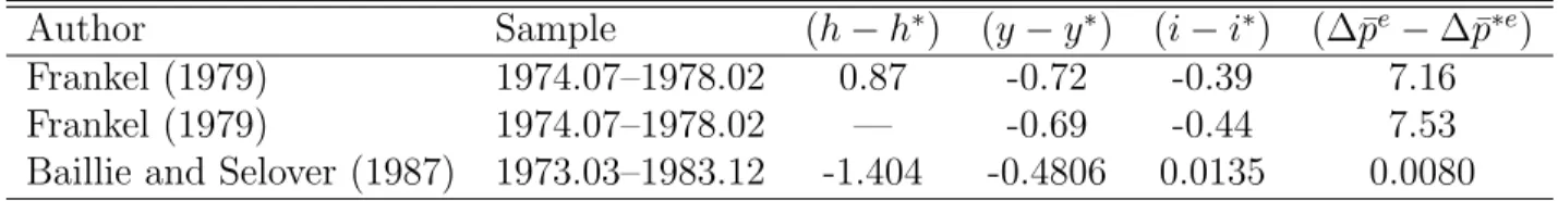
The first row of table 7.3 contains some coefficients estimates by Frankel (1979) for the DEM/USD exchange rate.9 All coefficients have the correct sign and are of plausible
size. In his initial (OLS) estimation, he found all estimated coefficients significant except for the interest rate coefficient. After some technical corrections (for serial correlation in the residuals and for possible regressor endogeneity) he also found a significant interest rate semi-elasticity. Frankel’s results were seen as exciting initial support for the real interest rate differential model. Note that Frankel (1979) proxied expected inflation by long-term interest rates, so his empirical implementation can be seen as considering the role of long-term and short-term interest rates.
9Frankel’s ordinary least squares (OLS) results are reported in the table. He assumesrp= 0. His reported coefficients on interest rates and expected inflation have been divided by four to correspond to coefficients on annual rates.
Author Sample (h−h∗) (y−y∗) (i−i∗) (∆¯pe−∆¯p∗e)
Frankel (1979) 1974.07–1978.02 0.87 -0.72 -0.39 7.16
Frankel (1979) 1974.07–1978.02 — -0.69 -0.44 7.53
Baillie and Selover (1987) 1973.03–1983.12 -1.404 -0.4806 0.0135 0.0080
Table 7.3: RID Model of DEM/USD Exchange Rate
The second row of table 7.3 contains additional results coefficient estimates reported by Frankel.10 This time, Frankel imposed a coefficient of one on the relative money supplies, as implied by his theoretical model. Frankel notes that imposing this constraint addresses worries that central banks may vary money supplies in response to exchange rates, and may also improve the estimation if money demand shocks are important. However, the remaining coefficients are little changed, suggesting perhaps that these problems were not important at the time.
Later applications of the model proved less supportive. For example, extending the data set, Baillie and Selover (1987) found Frankel’s earlier results no longer applied. The relative money supply and interest rate coefficients were significant but of the wrong sign. (Significant, perversely-signed coefficients on relative money supply were a common finding in later work—a significant problem for any “monetary” approach.) The coefficients on relative income and inflation had the right signs but are insignificant. Correcting for serial correlation in the residuals eliminated the sign difficulties, but then all these coefficients were insignificant. Baillie and Selover also found similar problems for other countries.
The real interest differential model has been widely tested. Although some initial research in the late 1970s generated promising results, extension of the sample period past 1978 typi-cally generated insignificant, negatively signed coefficients on relative money supplies. (The theory predicts unity.) Backus (1984) is an exception in supporting this for Canadian/US data. This problem may be due to money supply endogeneity. It has been observed that there is certainly some simultaneity problem, since both i and h are regressors but at most
10As in the reprint of this article in?, the interest rate and inflation semi-elasticities reported in Frankel (1979) have been divided by 4, so that they can be read as responses to changes inannual rates of return.
7.4. MONEY MARKET CONSIDERATIONS 23
one can be targetted by the monetary authority. Taking an example from Pentecost p.71, suppose depreciation raises i thereby reducing h. Another problem is that the residuals showed considerable serial correlation.
The real interest differential model can be modified to allow endogenous terms of trade. For example, ? include changes in the long run real exchange rate in their portfolio balance model. Their approach was simply to replace long run PPP with an expected long run real exchange rate, qe
t. Algebraically, the PPP equation is replaced with
¯
set =qet+pet−p∗et
The result is very similar to the Frankel real interest differential model.
st=qet +ht−h∗t −φ(yt−yt∗) +λ(∆p e t+1−∆p ∗e t+1)− 1 θ[(it−∆p e t+1)−(i ∗ t −∆p ∗e t+1)]− 1 θrp
Finally, there has been some attempts to endogenize the risk premium by linking it to relative asset supplies. This yields a model known as the portfolio balance model. (See chapter 10 for a discussion of this model.)
7.4
Money Market Considerations
As discussed in section 7.1.2, when prices are sticky we expect that monetary policy has liquidity effects. That is, we expect that expansionary monetary policy can lower the real interest rate in the short run. The simplest way to model these is with our standard repre-sentation of money market equilibrium.
Suppose the money market remains in constant equilibrium, which we continue to char-acterize as follows.
H
P =L(i, Y) (7.20)
on the price level to clear the money market. For the money market to clear when prices are sticky, changes in the money supply must be accommodated by changes in the interest rate.
Recall that the covered interest parity relationship and regressive expectations imply the negative relationship between the spot rate and the interest rate given by (7.3), which is repeated here for convenience.
i−i∗−rp =−θ δs
Solving this equation for the interest rate yields (7.21).
i=i∗+rp −θ δs (7.21)
We can use (7.21) to substitute for the interest rate in (7.20), yielding (7.22).
H
P =L(i
∗
+rp−θ δs, Y) (7.22)
If prices and income are “stuck” at their pre-shock values in the short run, a nominal money supply increase initially increases the real money supply. This lowers the equilibrium interest rate, which will generate disequilibrium capital outflows unless the exchange rate depreciates so far that it is expected to appreciate toward its long-run equilibrium value.
Equation (7.22) determines a unique spot rate that is compatible with any given price level. Recall that covered interest parity implies that the interest rate will be lower when the exchange rate is expected to appreciate. We also saw that, under regressive expectations, the exchange rate will be expected to appreciate when it is high (i.e., above its long-run equilibrium rate). Together these imply that the interest rate will be lower when the exchange rate is higher. We have now added a link between the price level and the interest rate. At a lower price level, there are higher real balances and the money market must therefore clear at a lower domestic interest rate. When combined with covered interest parity and regressive expectations, this yields a negative relationship between the price level and the exchange
7.4. MONEY MARKET CONSIDERATIONS 25
rate. Covered interest parity tells us this low interest rate must be offset by expected appreciation of the domestic currency. Capital outflows in response to the low interest rate will depreciate the currency until its expected future appreciation is just enough to offset the interest differential. So the combinations of P and S such that the assets markets clear can be represented by the LM curve in figure 7.8.
S1 s S2 s P S H H H H H H H H H H H H H H H H H H H H H H H H H H H HH LM LM0 P0
Figure 7.8: Exchange Rate Determination with Sticky Prices
The effects of an increase in the money supply can be represented as as shift out of the LM curve to LM0. At a given price level, such as P0, an increase in the nominal money
supply creates an increase in the real money supply. For the money market to clear, the interest rate must fall. Interest parity then requires expected appreciation of the domestic currency, which under regressive expectations implies a large depreciation of the spot rate.
We can fill in the story behing the exchange rate depreciation. With low domestic interest rates and high capital mobility, a large captial outflow will be initiated. This capital outflow drives up the spot rate. Only when the spot rate has risen far enough that it creates an adequate expectation of future appreciation does the incentive for capital outflow cease.
7.4.1
Overshooting with Sticky Prices
We have seen how exchange rates are determined when prices are sticky. Let us review why this exchange rate movement is overshooting. First we need to characterize the
full-s ¯ S1 A s C ¯ S2 s B Ssr P S H H H H H H H H H H H H H H H H H H H H H H H H H H H H H LM LM0 P0
Figure 7.9: Exchange Rate Overshooting with Sticky Prices
equilibrium outcomes. We turn to the equilibrium described by the simple Classical model of chapter 6. In the Classical model, money is neutral: a one-time, permanent change in the money supply leads to a proportional change in prices and the exchange rate. We will now adopt this as our long-run description of the effect of a money supply change. Long-run neutrality of money implies that in the long Long-run the price level and the exchange rate increase in proportion to the money supply increase, so that all real variables are unaffected. We will represent this by point A in figure 7.9. Intuitively, if the Classical model adequately represents the long-run behavior of the exchange rate, we expect that a money supply increase should eventually lead to a proportional change in the exchange rate, a proportional change in the price level, and no change in the real exchange rate. A line from the origin through point A has a constant real exchange rate. (It is just our IS curve from the simple Classical model of chapter 6.) Point C must therefore represent the new long-run equilibrium, while point B represents the run response to the money supply increase. Clearly the short-run exchange-rate movement is greater than required to reach the long-short-run exchange rate. The excessive movement, Ssr−S¯2, is the exchange rate overshoot.
The Algebra
As in section 7.1.3, the algebra will be a matter of covered interest parity, regressive expecta-tions, and liquidity effects. This time, however, the liquidity effects are explicitly motivated
7.4. MONEY MARKET CONSIDERATIONS 27
by sticky prices and income, along with continuous money market equilibrium.
Recall from section 7.1.3 that covered interest parity and regressive expectations imply (7.6), which we repeat here for convenience.
s= ¯s− 1
θ(i−i
∗−
∆¯se−rp) (7.6)
We add money market considerations by turning to our usual representation of money market equilibrium.
h−p=φy−λi (7.23)
Solving (7.23) fori yields (7.24).
i=−1
λ(h−p−φy) (7.24)
Together (7.6) and (7.24) imply
s = ¯s+ 1
θλ[h−p−φy+λ(∆¯s
e+i∗
+rp)] (7.25)
Equation (7.25) therefore combines three ingredients: covered interest parity, regressive ex-pectations, and money market equilibrium.
Now consider a one-time, permanent change in the money supply, dh. We continue to treat the foreign interest rate and the risk premium as exogenous. So we get
ds dh = ds¯ dh + 1 θλ(1− dp dh −φ dy dh) (7.26)
immediately. ds dh = d¯s dh + 1 θλ > d¯s dh
The long-run neutrality of money implies d¯s =dh. So under long-run neutrality of money, we can write our overshooting result as
ds
dh = 1 +
1
θλ
Here is another way to characterize the same result. Using the notationδs=s−s¯, (7.25) implies
δs=− 1
λθ(δp+φδy) (7.27)
Starting from a steady state and increasing h (once, permanently) by one unit (at t = 0, say) implies in any model where prices and income are sticky and money is neutral in the long run that δp0 = −1 and δy0 = 0. The implication is that the exchange rate overshoots
(that δs0 >0) since
δs0 =
1
λθ (7.28)
Note that with a smaller the speed of adjustment (θ), or a less interest sensitive is the demand for money (λ), the larger is overshooting of the exchange rate. Be sure you can explain this result intuitively.
7.5. SIMPLE EMPIRICAL CONSIDERATIONS 29
Source: Rogoff (2002)
Figure 7.10: Interest Differential (rDE−rU S) and USD-DEM Exchange Rate
Source: Rogoff (2002)
7.5
Simple Empirical Considerations
7.5.1
Can We See the CIPRE Relationship?
Any CIPRE relationship in the data proves empirically elusive. Meese and Rogoff (1988) fail to find a statistically significant relationship between the real exchange rate and the real interest rate. Furthermore, while time series plots appear promising for some countries, as in the German data illustrated in Figure 7.10, they do not for other countries, as in the UK data illustrated in Figure 7.11.
Taylor (1995) gives a somewhat more optimistic assessment. By considering the dollar against an aggregate of G-10 countries, he illustrates a fairly good long-term relationship between the real exchange rate and real interest rates, even though the short-run fluctuations diverge. This is illustrated in Figure 7.12.
Source: Taylor (1995)
7.5. SIMPLE EMPIRICAL CONSIDERATIONS 31
Source: Rogoff (2002)
Figure 7.13: Spot and Forward Rates
7.5.2
Forward Rates
Flood (1981) points out that the overshooting model suggests that forward rates should be less responsive to monetary policy shocks than spot rates. Typically however they move very closely together, as illustrated in Figure 7.13.
Does the empirical failure of the Mundell-Fleming-Dornbusch model mean that we have to reject it as a useful tool for policy analysis? Not at all. First, . . . the broader usefulness of the Mundell-Fleming-Dornbusch model goes well beyond the overshooting prediction. It is a generalized framework for thinking about international macroeconomic policy. Second, . . . the model does not necessarily predict overshooting when output is endogenous. Third, . . . consumption typi-cally appears in place of output in the money demand equations; this change also tilts the balance away from overshooting. . . . the apparent ability of the Dorn-busch model to describe the trajectory of the exchange rate after major shifts in
monetary policy is more than enough reason for us to press ahead and look more deeply at its underlying theoretical structure.
Rogoff (2002)
7.5.3
VAR Analysis
Eichenbaum and Evans
The most famous VAR study of overshooting is probably Eichenbaum and Evans (1995). They create a variety of VAR models for a number of countries. As one measure of monetary policy they used the ratio of nonborrowed reserves to total reserves, which they call NBRX. (They also considered shocks to the federal funds rate.) Their sample is 1974.01–1990.05. In their first reported set of results, the variables are
Y: US industrial production P: US CPI
NBRX: non-borrowed reserves to total reserves i∗−i: interest differential
S orQ: nomain or real exchange rate (two versions)
All variables were converted to logs except the interest differential. The countries considered (in separate VARs) were Japan, Germany, Italy, France, and the UK.
Results were very similar for the real and nominal exchange rate. (No surprise: we already know these are highly correlated.) A monetary contraction leads to a quick appreciation, as predicted by the overshooting model. But this appreciation continues over time before being reversed, a pattern that is sometimes called delayed overshooting. Monetary shocks look to be an important determinant of exchange rate dynamics. Additionally, they produce sustained deviations from covered interest parity.
7.6. CONCLUSION 33
Figure 7.14:
The long hump in exchange rate response has been found in numerous studies. Scholl and Uhlig (2008) refer to it as thedelayed overshooting puzzle. As we will see, however, the overshooting puzzle is not much of a puzzle in the face of anticipated policy changes.
7.6
Conclusion
The simple overshooting approach to flexible exchange rates has two key constituents: cov-ered interest parity and regressive expectations. The result is a very simple model of ex-change rate determination that explains one of the key stylized facts of flexible exex-change rate regimes: exchange volatility is high relative to the volatility of the underlying fundamentals. Early empirical tests yielded encouraging support for the overshooting approach. Later
tests proved much less satisfactory. In contrast with the monetary approach, the fact that much of the empirical work has used small samples of monthly data for countries with low average inflation rates does not raise our hopes. The overshooting approach was intended to augment the monetary approach’s description of the fundamental long-run influences on the exchange rate with a story about short-run dynamics. The empirical failures of the overshooting approach are therefore extremely disappointing.
Nevertheless, the overshooting approach appears to offer some important insights. It suggests one reason why the exchange rate can be much more volatile than than the under-lying fundamentals, which is clearly true with actual exchange rates. It also predicts that monetary tightening will lead to a rise in the real interest rate and an appreciation of the real exchange rate. Countries that move from high-inflation to low-inflation policy regimes often experience such effects (Rogoff, 1999).
Predictions of the overshooting approach include the following. The most important predictions is that an increase in the domestic money supply leads to a proportional depre-ciation of the spot exchange rate in the long run, but in the short run the depredepre-ciation is more than proportional. Furthermore, in the short run there will be a decline in the real interest rate, a depreciation of the real exchange rate, and a corresponding improvement in the trade balance. Recalling our work on the Classical model, we know that the long-run effects of an increase in domestic income are somewhat more complicated, since this will tend to appreciate the exchange rate through the money market while depreciating the real exchange rate through the goods market.
Expansionary monetary policy might be represented either as a change in the level or as a change in the growth rate of the money supply. In each case, the policy change may be a complete surprise or it may be anticipated. This leads to four possible scenarios. Once again, a primary lesson is that any effort to model exchange rates must pay careful attention to the role of expectations.
35
Problems for Review
1. Why do regressive expectations and convered interest parity imply a negative relation-ship between the interest rate and the exchange rate?
2. What is exchange rate overshooting and why is it important?
3. Why does the combination of regressive expectations, convered interest parity, and liquidity effects imply overshooting in response to money supply changes?
4. How does figure 7.2 change if we add a “core-inflation” rate to the expected rate of depreciation?
5. Consider figure 7.3. Can an exogenous change in the risk premium cause overshooting?
6. Why does the combination of regressive expectations, convered interest parity, sticky prices, and money market equilibrium imply overshooting in response to money supply changes?
7. In the late 1970s, Argentina set its exchange rate according to a tablita: a series of small, preannounced devaluations. What does this imply for the nominal interest rate differential? At the same time the real interest rate in Argentina was high: what does this imply about expected depreciation?
8. ? develops the link between real interest differentials and market perception of ex-change rate overvaluation. In mid-1984, the real interest differential on U.S. 10 year bonds was around 3.5%/year. What does that imply for expected depreciation of the dollar. Let us say 10 years is enough time to return to PPP: what does the real interest differential say about the extent of overvaluation of the dollar?
7.7
Overshooting Price Dynamics in Continuous Time
Dornbusch’s explanation shocked and delighted researchers because he showed how overshooting did not necessarily grow out of myopia or herd behavior in markets.
Rogoff (2002)
This section characterizes the sticky price dynamics in continuous time, which is a com-mon theoretical treatment. The algebraic details in this section may be skipped by all MA students.
7.7.1
Regressive Expectations
Recall the basic (partially reduced) structural relationships of the model
H P =L(i ∗− θ δs, Y) (7.29) AD =AD(i∗−θ δs, Y, G, SP∗/P) (7.30) ∆p=f AD(i∗−θ δs, Y, G, SP∗/P) Y (7.31)
For example, consider the implied movement around the long run equilibrium point (¯p,s¯). Defineδp =p−p¯and δs=s−s¯, the deviations of prices and the exchange rate from their long run level. Then rewrite money market equilibrium and the price adjustment equation in deviation form. This turns (7.29) and (7.31) into (7.32) and (7.33).
−δp=λθδs (7.32)
Dδp=π(ρ+σθ)δs−πρδp (7.33)
You will recognize this as a linear homogeneous first order differential equation system. One easy way to solve it is to solve (7.32) for δs, plug this solution into (7.33), and solve
7.7. DORNBUSCH (1976) 37
the resulting differential equation in δp. The dynamics of δs will then be found by time differentiating (7.32) after substituting your solution for δp.
Dδp=−π(ρ+σθ)/λθδp−πρδp =−π[ρ(1 + 1/λθ) +σ/λ]δp =Aδp (7.34) Therefore δp=δp0eAt (7.35)
Note that it makes sense to solve this in terms ofδp0, sincepis a predetermined variable.
Since A <0, we are assured of the stability of the system.
It is also possible to attack the solution directly using the adjoint matrix technique. First, let’s write (7.32) and (7.33) in matrix form using the differential operator.
−1 −λθ D+πρ −π(ρ+σθ) δs δp = 0 (7.36)
We can solve the characteristic equation
λθD+π(ρλθ+ρ+σθ) = 0 (7.37)
for the unique characteristic root
D1 = −π(ρλθ+ρ+σθ)/λθ
= −π[ρ(1 + 1/λθ) +σ/λ]
< 0
the general solution to (7.32) and (7.33). δp δs =kexp{D1t} λθ −1 (7.38)
Note that this involves a single arbitrary constant, so that we cannot offer arbitrary initial conditions for bothδp andδs. We supply an initial condition for the predetermined variable
δp0, since prices cannot move instantaneously to clear the goods market. In contrast, the
exchange rate can jump to maintain constant asset market equilibrium.
7.7.2
Rational Expectations
In this section we replace the regressive expectations hypothesis with the rational expec-tations hypothesis. Since there is no uncertainty in this model, the rational expecexpec-tations hypothesis implies ˙se = ˙s. Given uncovered interest parity (i = i∗ + ˙s), we can then use
the money market equilibrium condition to express the rate of exchange rate depreciation in terms of p.
h−p=φy−λ(i∗+ ˙s) (7.39)
As we have laid out the model, ˙s = 0 in the long run. So we know
h−p¯=φy−λi∗ (7.40)
Comparing the short-run and long-run we see
p−p¯=λs˙ (7.41)
which implies
˙
7.7. DORNBUSCH (1976) 39 p ¯ p s ˙ s<0 s>˙ 0 ˙ s=0
Figure 7.15: The ˙s= 0 Locus
Our basic descriptions of the goods market and of price adjustment are unchanged, so under the rational expectation hypothesis
˙
p=π[ρ(s−p)−σ(i∗+ ˙s) +g−y] (7.43)
Equivalently, in terms of deviations from the equilibrium values (again recalling that ˙
s= 0 in the long run),
˙
p=π[ρ(s−¯s)−ρ(p−p¯)−σs˙] (7.44)
Our solution for ˙s allows us to rewrite this as11
˙
p=−a(p−p¯) +b(s−s¯) (7.45)
making it simple to graph the ˙p= 0 locus.
11Herea=πρ+πσ/λandb=πρ, and the implied slope along the ˙p= 0 isocline is (ds/dp)| ˙
p s ˙ p>0 p<˙ 0 ˙ p=0
Figure 7.16: The ˙p= 0 Locus
Once again, we can solve the homogeneous system12
D+a −b −1/λ D p−p¯ s−s¯ = 0 (7.46)
by the adjoint matrix technique. First solve the characteristic equation D2+aD−b/λ = 0
for the two roots D1 and D2, where D1 < D2.
D1, D2 =
−a±p
a2+ 4b/λ
2 (7.47)
This clearly gives us one positive and one negative real root. Thus the following solution blows up unless η2 = 0. p−p¯ s−s¯ =η1exp{D1t} D1 1/λ +η2exp{D2t} D2 1/λ (7.48)
It is typical for macromodels with flexible asset prices to exhibit such “saddle-point instability.” Early discussions of this situation suggested that the convergent arm should be
12There is no need to substitute for ˙sas we have done here. (Show this as a homework by working through the solution without this substitution.)
7.7. DORNBUSCH (1976) 41
selected from all the possible dynamic paths as the only economically “reasonable” solution, and a subsequent literature provided some more sophisticated justifications for this general procedure. Selecting the covergent arm is of course the same as settingη2 = 0 in our solution.
In addition to ruling out behavior that many economists consider somewhat perverse–e.g., hyperinflation with a constant money stock–limiting our attention to the convergent arm allows us to make predictions with the model that would otherwise be impossible. For although the price level is predetermined, the exchange rate may potentially jump to any
7.7.3
Unanticipated Policy Shocks
If we assume the exchange rate jumps to the convergent arm, then we know that the exchange rate overshoots in response to an unanticipate monetary shock. We also know that inflation and exchange rate appreciation are correlated. So we get some strong potentially testable predictions. s p sLR p0 sSR ˙ s=0 ˙ p=0
Figure 7.17: Rational Expectations and Overshooting
So with rational expectations, we will also see the same overshooting phenomenon. Comment: We can readily describe the slope of the convergent arm once we note that for any initial δp0 we can solve η1 =δp0/D1. This implies δs0 =δp0/λD1. But we can just
think of the slope of the convergent arm as δs0/δp0 = 1/λD1. (Why?)
Comment: Recall ¯ph = 1. If we are in a steady state at the time of the monetary
shock, ¯ph = 1 implies δp0 = −dh. We can then solve for η1 = −dh/D1. This gives us δs0 = −dh/λD1 > 0. The positive sign indicates overshooting: s has risen above its new
long run value.
As illustrated in Figure 7.17, unanticipated fiscal shocks do not produce interesting dy-namics. However, we again see the twin deficits phenomenon.
7.7. DORNBUSCH (1976) 43 s p ∆s ˙ s=0 ˙ p=0 p˙0=0
7.7.4
Anticipated Shocks
Bibliography
Backus, D. (1984, November). “Empirical Models of the Exchange Rate: Separating the Wheat from the Chaff.” Canadian Journal of Economics 17(4), 824–46.
Baillie, R.T. and D.D. Selover (1987). “Cointegration and Models of Exchange Rate Deter-mination.” International Journal of Forecasting 3(1), 43–52.
Dornbusch, Rudiger (1976, December). “Expectations and Exchange Rate Dynamics.” Jour-nal of Political Economy 84(6), 1161–76.
Duarte, Margarida (2003, Summer). “The Euro and Inflation Divergence in Europe.” Federal Reserve Bank of Richmond Economic Quarterly 89(3), 53–70.
Eichenbaum, Martin and Charles Evans (1995, November). “Some Empirical Evidence of the Effects of Shocks to Monetary Policy on Exchange Rates.” Quarterly Journal of Economics 110(4), 975–1009.
Flood, Robert P. (1981, Autumn). “Explanations of Exchange-Rate Volatility and Other Em-pirical Regularities in Some Popular Models of the Foreign Exchange Market.” Carnegie-Rochester Conference Series on Public Policy 15, 219–249. Available as NBER Working Paper 625, February 1981.
Florentis, G., D.V. Gordon, and P. Huber (1994, Autumn). “Monetary Models of the Canadian-U.S. Exchange Rate: A Reexamination of the Empirical Evidence, 1971– 1986.” Quarterly Journal of Business and Economics 33(4), 27–43.
Frankel, Jeffrey and Kenneth Froot (1987, March). “Using Survey Data to Test Stan-dard Propositions Regarding Exchange Rate Expectations.” American Economic Re-view 77(1), 133–53.
Frankel, Jeffrey A. (1979, September). “On the Mark: A Theory of Floating Exchange Rates Based on Real Interest Rate Differentials.” American Economic Review 69(4), 610–22.
Meese, Richard A. and Kenneth Rogoff (1988). “Was It Real? The Exchange Rate-Interest Differential Relation over the Modern Floating-Rate Period.” Journal of Finance 43(4), 933–948.
Rogoff, Kenneth (1999, November). “Monetary Models of Dollar/Yen/Euro Nominal Ex-change Rates: Dead or Undead.” Economic Journal 109(459), F655–9.
Rogoff, Kenneth (2002, January). “Dornbusch’s Overshooting Model After Twenty-Five Years.
Scholl, Almuth and Harald Uhlig (2008). “New Evidence on the Puzzles: Results from Ag-nostic Identification on Monetary Policy and Exchange Rates.” Journal of International Economics 76, 1–13.
Taylor, John B. (1995, Fall). “The Monetary Transmission Mechanism: An Empirical Frame-work.” Journal of Economic Perspectives 9(4), 11–26.
Driskill, R.A. and S.M. Sheffrin, 1981, “On the Mark: Comment”, AER 71, 1068–74. Frankel, J.A., 1983, “Monetary and Portfolio-Balance Models of Exchange Rate
De-termination,” in J. Bhandari and B. Putnam (eds), Economic Interdependence and Flexible Exchange Rates (Cambridge, MA: MIT Press)
Frankel, J.A., 1984, “Tests of Monetary and Portfolio-Balance Models of Exchange Rate Determination,” in J. Bilson and R. Marston (eds), Exchange Rate Theory and Practice (Chicago: University of Chicago Press)
BIBLIOGRAPHY 47 Frankel, J.A., 1992, “Update to Monetary and Portfolio-Balance Models of Exchange Rate Determination,” in John Letiche (ed),International Economic Policies and Their Theoretical Foundations: A Sourcebook 2nd Edition (London: Academic Press)