Recent Advances of Large-Scale
Linear Classification
This paper is a survey on development of optimization methods to construct linear
classifiers suitable for large-scale applications; for some data, accuracy is
close to that of nonlinear classifiers.
By
G u o - X u n Y u a n
,
C h i a - H u a H o , a n d C h i h - J e n L i n ,
Fellow IEEE
ABSTRACT
|
Linear classification is a useful tool in machine learning and data mining. For some data in a rich dimensional space, the performance (i.e., testing accuracy) of linear classi-fiers has shown to be close to that of nonlinear classiclassi-fiers such as kernel methods, but training and testing speed is much faster. Recently, many research works have developed efficient optimization methods to construct linear classifiers and ap-plied them to some large-scale applications. In this paper, we give a comprehensive survey on the recent development of this active research area.KEYWORDS
|
Large linear classification; logistic regression; multiclass classification; support vector machines (SVMs)I .
I N T R O D U C T I O N
Linear classification is a useful tool in machine learning and data mining. In contrast to nonlinear classifiers such as kernel methods, which map data to a higher dimen-sional space, linear classifiers directly work on data in the original input space. While linear classifiers fail to handle some inseparable data, they may be sufficient for data in a rich dimensional space. For example, linear classifiers
have shown to give competitive performances on docu-ment data with nonlinear classifiers. An important ad-vantage of linear classification is that training and testing procedures are much more efficient. Therefore, linear classification can be very useful for some large-scale appli-cations. Recently, the research on linear classification has been a very active topic. In this paper, we give a compre-hensive survey on the recent advances.
We begin with explaining in Section II why linear classification is useful. The differences between linear and nonlinear classifiers are described. Through experiments, we demonstrate that for some data, a linear classifier achieves comparable accuracy to a nonlinear one, but both training and testing times are much shorter. Linear clas-sifiers cover popular methods such as support vector machines (SVMs) [1], [2], logistic regression (LR),1and others. In Section III, we show optimization problems of these methods and discuss their differences.
An important goal of the recent research on linear classification is to develop fast optimization algorithms for training (e.g., [4]–[6]). In Section IV, we discuss issues in finding a suitable algorithm and give details of some representative algorithms. Methods such as SVM and LR were originally proposed for two-class problems. Although past works have studied their extensions to multiclass problems, the focus was on nonlinear classification. In Section V, we systematically compare methods for multi-class linear multi-classification.
Linear classification can be further applied to many other scenarios. We investigate some examples in Section VI. In particular, we show that linear classifiers can be effectively employed to either directly or indirectly approximate nonlinear classifiers. In Section VII, we Manuscript received June 16, 2011; revised November 24, 2011; accepted February 3,
2012. Date of publication March 30, 2012; date of current version August 16, 2012. This work was supported in part by the National Science Council of Taiwan under Grant 98-2221-E-002-136-MY3.
G.-X. Yuanwas with the Department of Computer Science, National Taiwan University, Taipei 10617, Taiwan. He is currently with the University of California Davis, Davis, CA 95616 USA (e-mail: r96042@csie.ntu.edu.tw).
C.-H. HoandC.-J. Linare with the Department of Computer Science, National Taiwan University, Taipei 10617, Taiwan (e-mail: b95082@csie.ntu.edu.tw; cjlin@csie.ntu.edu.tw).
Digital Object Identifier: 10.1109/JPROC.2012.2188013
1It is difficult to trace the origin of logistic regression, which can be dated back to the 19th century. Interested readers may check the investigation in [3].
discuss an ongoing research topic for data larger than memory or disk capacity. Existing algorithms often fail to handle such data because of assuming that data can be stored in a single computer’s memory. We present some methods which try to reduce data reading or communi-cation time. In Section VIII, we briefly discuss related topics such as structured learning and large-scale linear regression.
Finally, Section IX concludes this survey paper.
I I .
W H Y I S L I N E A R
C L A S S I F I C A T I O N U S E F U L ?
Given training dataðyi;xiÞ 2 f1;þ1g Rn,i¼1;. . .;l,
where yi is the label and xi is the feature vector, some
classification methods construct the following decision function:
dðxÞ wTðxÞ þb (1)
where w is the weight vector and b is an intercept, or called the bias. Anonlinearclassifier maps each instancex
to a higher dimensional vector ðxÞ if data are not lin-early separable. If ðxÞ ¼x (i.e., data points are not mapped), we say (1) is alinearclassifier. Because nonlin-ear classifiers use more features, generally they perform better than linear classifiers in terms of prediction accuracy.
For nonlinear classification, evaluatingwTðxÞcan be
expensive because ðxÞ may be very high dimensional. Kernel methods (e.g., [2]) were introduced to handle such a difficulty. Ifw is a linear combination of training data, i.e.,
wX
l
i¼1
iðxiÞ; for some A2Rl (2)
and the following kernel function can be easily calculated:
Kðxi;xjÞ ðxiÞTðxjÞ
then the decision function can be calculated by
dðxÞ X
l
i¼1
iKðxi;xÞ þb (3)
regardless of the dimensionality ofðxÞ. For example
Kðxi;xjÞ xTixjþ1
2
(4)
is the degree-2 polynomial kernel with
ðxÞ ¼ 1;pffiffiffi2x1;. . .; ffiffiffi 2 p xn;. . .x21;. . .x2n; ffiffiffi 2 p x1x2; h ffiffiffi 2 p x1x3;. . .; ffiffiffi 2 p xn1xn i 2Rðnþ2Þðnþ1Þ=2: (5) This kernel trick makes methods such as SVM or kernel LR practical and popular; however, for large data, the training and testing processes are still time consuming. For a kernel like (4), the cost of predicting a testing instancexvia (3) can be up toOðlnÞ. In contrast, without using kernels,wis available in an explicit form, so we can predict an instance by (1). WithðxÞ ¼x
wTðxÞ ¼wTx
costs only OðnÞ. It is also known that training a linear classifier is more efficient. Therefore, while a linear clas-sifier may give inferior accuracy, it often enjoys faster training and testing.
We conduct an experiment to compare linear SVM and nonlinear SVM [with the radial basis function (RBF) ker-nel]. Table 1 shows the accuracy and training/testing time. Generally, nonlinear SVM has better accuracy, especially for problems cod-RNA,2 ijcnn1, covtype, webspam, andMNIST38. This result is consistent with the theoret-ical proof that SVM with RBF kernel and suitable parameters gives at least as good accuracy as linear kernel [10]. However, for problems with large numbers of fea-tures, i.e., real-sim, rcv1, astro-physic, yahoo-japan, andnews20, the accuracy values of linear and nonlinear SVMs are similar. Regarding training and testing time, Table 1 clearly indicates that linear classifiers are at least an order of magnitude faster.
In Table 1, problems for which linear classifiers yield comparable accuracy to nonlinear classifiers are all docu-ment sets. In the area of docudocu-ment classification and natural language processing (NLP), a bag-of-word model is commonly used to generate feature vectors [11]. Each feature, corresponding to a word, indicates the existence
2
In this experiment, we scaledcod-RNAfeature wisely to½1;1
of the word in a document. Because the number of fea-tures is the same as the number of possible words, the dimensionality is huge, and the data set is often sparse. For this type of large sparse data, linear classifiers are very useful because of competitive accuracy and very fast train-ing and testtrain-ing.
I I I .
B I N A R Y L I N E A R
C L A S S I F I C A T I O N M E T H O D S
To generate a decision function (1), linear classification involves the following risk minimization problem:
min
w;b fðw;bÞ rðwÞ þC
Xl i¼1
ðw;b;xi;yiÞ (6)
whererðwÞis the regularization term and ðw;b;x;yÞis the loss function associated with the observation ðy;xÞ. ParameterC>0 is user specified for balancingrðwÞand the sum of losses.
Following the discussion in Section II, linear classifi-cation is often applied to data with many features, so the bias termbmay not be needed in practice. Experiments in [12] and [13] on document data sets showed similar performances with/without the bias term. In the rest of this paper, we omit the bias termb, so (6) is simplified to
min
w fðwÞ rðwÞ þC
Xl i¼1
ðw;xi;yiÞ (7)
and the decision function becomesdðxÞ wTx.
A. Support Vector Machines and Logistic Regression In (7), the loss function is used to penalize a wrongly classified observation ðx;yÞ. There are three common
loss functions considered in the literature of linear classification L1ðw;x;yÞ maxð0;1ywTxÞ (8) L2ðw;x;yÞ maxð0;1ywTxÞ 2 (9) LRðw;x;yÞ log1þeywTx: (10)
Equations (8) and (9) are referred to as L1 and L2 losses, respectively. Problem (7) using (8) and (9) as the loss function is often called L1-loss and L2-loss SVM, while problem (7) using (10) is referred to as logistic regression (LR). Both SVM and LR are popular classification meth-ods. The three loss functions in (8)–(10) are all convex and nonnegative. L1 loss is not differentiable at the point ywTx¼1, while L2 loss is differentiable, but not twice
differentiable [14]. For logistic loss, it is twice differentia-ble. Fig. 1 shows that these three losses are increasing functions ofywTx. They slightly differ in the amount of penalty imposed.
B. L1 and L2 Regularization
A classifier is used to predict the labelyfor a hidden (testing) instancex. Overfitting training data to minimize
Fig. 1.Three loss functions:L1,L2, andLR. Thex-axis isywTx.
Table 1Comparison of Linear and Nonlinear Classifiers. For Linear, We Use the SoftwareLIBLINEAR[7], While for Nonlinear We UseLIBSVM[8] (RBF Kernel). The Last Column Shows the Accuracy Difference Between Linear and Nonlinear Classifiers. Training and Testing Time Is in Seconds. The Experimental Setting Follows Exactly From [9, Sec. 4]
the training loss may not imply that the classifier gives the best testing accuracy. The concept of regularization is introduced to prevent from overfitting observations. The following L2 and L1 regularization terms are commonly used: rL2ðwÞ 1 2kwk 2 2¼ 1 2 Xn j¼1 w2j (11) and rL1ðwÞ kwk1¼ Xn j¼1 jwjj: (12)
Problem (7) with L2 regularization and L1 loss is the standard SVM proposed in [1]. Both (11) and (12) are convex and separable functions. The effect of regulariza-tion on a variable is to push it toward zero. Then, the search space ofwis more confined and overfitting may be avoided. It is known that an L1-regularized problem can generate a sparse model with few nonzero elements inw. Note thatw2=2 becomes more and more flat toward zero, but jwj is uniformly steep. Therefore, an L1-regularized variable is easier to be pushed to zero, but a caveat is that (12) is not differentiable. Because nonzero elements inw
may correspond to useful features [15], L1 regularization can be applied for feature selection. In addition, less memory is needed to storewobtained by L1 regularization. Regarding testing accuracy, comparisons such as [13, Suppl. Mater. Sec. D] show that L1 and L2 regularizations generally give comparable performance.
In statistics literature, a model related to L1 regular-ization is LASSO [16] min w Xl i¼1 ðw;xi;yiÞ subject to kwk1K (13)
whereK>0 is a parameter. This optimization problem is equivalent to (7) with L1 regularization. That is, for a given C in (7), there exists K such that (13) gives the same solution as (7). The explanation for this relationship can be found in, for example, [17].
Any combination of the above-mentioned two regular-izations and three loss functions has been well studied in linear classification. Of them, L2-regularized L1/L2-loss SVM can be geometrically interpreted as maximum margin classifiers. L1/L2-regularized LR can be interpreted in a Bayesian view by maximizing the posterior probability with Laplacian/Gaussian prior ofw.
A convex combination of L1 and L2 regularizations forms the elastic net [18]
reðwÞ kwk22þ ð1Þkwk1 (14)
where 2 ½0;1Þ. The elastic net is used to break the following limitations of L1 regularization. First, L1 regu-larization term is not strictly convex, so the solution may not be unique. Second, for two highly correlated features, the solution obtained by L1 regularization may select only one of these features. Consequently, L1 regularization may discard the group effect of variables with high correlation [18].
I V .
T R A I N I N G T E C H N I Q U E S
To obtain the modelw, in the training phase we need to solve the convex optimization problem (7). Although many convex optimization methods are available, for large linear classification, we must carefully consider some factors in designing a suitable algorithm. In this section, we first discuss these design issues and follow by showing details of some representative algorithms.
A. Issues in Finding Suitable Algorithms
• Data property. Algorithms that are efficient for some data sets may be slow for others. We must take data properties into account in selecting algo-rithms. For example, we can check if the number of instances is much larger than features, or vice versa. Other useful properties include the number of nonzero feature values, feature distri-bution, feature correlation, etc.
• Optimization formulation. Algorithm design is strongly related to the problem formulation. For example, most unconstrained optimization tech-niques can be applied to L2-regularized logistic regression, while specialized algorithms may be needed for the nondifferentiable L1-regularized problems.
In some situations, by reformulation, we are able to transform a nondifferentiable problem to be differentiable. For example, by letting w¼
wþw ðwþ;w0Þ, L1-regularized classifiers can be written as min wþ;w Xn j¼1 wþj þX n j¼1 wj þX l i¼1 ðwþw;xi;yiÞ subject to wþj ;wj 0; j¼1;. . .;n: (15)
However, there is no guarantee that solving a dif-ferentiable form is faster. Recent comparisons [13] show that for L1-regularized classifiers, methods directly minimizing the nondifferentiable form are often more efficient than those solving (15). • Solving primal or dual problems.Problem (7) hasn
variables. In some applications, the number of in-stanceslis much smaller than the number of fea-turesn. By Lagrangian duality, a dual problem of (7) haslvariables. Ifln, solving the dual form may be easier due to the smaller number of varia-bles. Further, in some situations, the dual problem possesses nice properties not in the primal form. For example, the dual problem of the standard SVM (L2-regularized L1-loss SVM) is the following quadratic program3: min A f DðAÞ 1 2A TQAeTA subject to 0iC 8i¼1;. . .;l (16)
whereQijyiyjxTixj. Although the primal objective
function is nondifferentiable because of the L1 loss, in (16), the dual objective function is smooth (i.e., derivatives of all orders are available). Hence, solving the dual problem may be easier than primal because we can apply differentiable optimization techniques. Note that the primal optimalwand the dual optimal A satisfy the relationship (2),4 so solving primal and dual problems leads to the same decision function.
Dual problems come with another nice property that each variable i corresponds to a training
instanceðyi;xiÞ. In contrast, for primal problems,
each variablewicorresponds to a feature.
Optimi-zation methods which update some variables at a time often need to access the corresponding instances (if solving dual) or the corresponding features (if solving primal). In practical applica-tions, instance-wise data storage is more common than feature-wise storage. Therefore, a dual-based algorithm can directly work on the input data without any transformation.
Unfortunately, the dual form may not be always easier to solve. For example, the dual form of L1-regularized problems involves general linear con-straints rather than bound concon-straints in (16), so solving primal may be easier.
• Using low-order or high-order information. Low-order methods, such as gradient or subgradient
methods, have been widely considered in large-scale training. They characterize low-cost update, low-memory requirement, and slow convergence. In classification tasks, slow convergence may not be a serious concern because a loose solution of (7) may already give similar testing performances to that by an accurate solution.
High-order methods such as Newton methods often require the smoothness of the optimization problems. Further, the cost per step is more expensive; sometimes a linear system must be solved. However, their convergence rate is superi-or. These high-order methods are useful for applications needing an accurate solution of problem (7). Some (e.g., [20]) have tried a hybrid setting by using low-order methods in the beginning and switching to higher order methods in the end. • Cost of different types of operations.In a real-world
computer, not all types of operations cost equally. For example, exponential and logarithmic opera-tions are much more expensive than multiplication and division. For training large-scale LR, because
exp=logoperations are required, the cost of this type of operations may accumulate faster than that of other types. An optimization method which can avoid intensiveexp=logevaluations is potentially efficient; see more discussion in, for example, [12], [21], and [22].
• Parallelization. Most existing training algorithms are inherently sequential, but a parallel algorithm can make good use of the computational power in a multicore machine or a distributed system. How-ever, the communication cost between different cores or nodes may become a new bottleneck. See more discussion in Section VII.
Earlier developments of optimization methods for lin-ear classification tend to focus on data with few features. By taking this property, they are able to easily train mil-lions of instances [23]. However, these algorithms may not be suitable for sparse data with both large numbers of instances and features, for which we show in Section II that linear classifiers often give competitive accuracy with nonlinear classifiers. Many recent studies have proposed algorithms for such data. We list some of them (and their software name if any) according to regularization and loss functions used.
• L2-regularized L1-loss SVM: Available approaches include, for example, cutting plane methods for the primal form (SVMperf [4], OCAS [24], and
BMRM [25]), a stochastic (sub)gradient descent method for the primal form (Pegasos [5], and
SGD[26]), and a coordinate descent method for the dual form (LIBLINEAR[6]).
• L2-regularized L2-loss SVM: Existing methods for the primal form include a coordinate descent method [21], a Newton method [27], and a trust 3
Because the bias termbis not considered, therefore, different from the dual problem considered in SVM literature, an inequality constraint
P
yii¼0 is absent from (16).
4However, we do not necessarily need the dual problem to get (2). For example, the reduced SVM [19] directly assumes thatwis the linear combination of a subset of data.
region Newton method (LIBLINEAR [28]). For the dual problem, a coordinate descent method is in the softwareLIBLINEAR[6].
• L2-regularized LR: Most unconstrained optimiza-tion methods can be applied to solve the primal problem. An early comparison on small-scale data is [29]. Existing studies for large sparse data in-clude iterative scaling methods [12], [30], [31], a truncated Newton method [32], and a trust region Newton method (LIBLINEAR [28]). Few works solve the dual problem. One example is a coordi-nate descent method (LIBLINEAR[33]).
• L1-regularized L1-loss SVM: It seems no studies have applied L1-regularized L1-loss SVM on large sparse data although some early works for data with either few features or few instances are available [34]–[36].
• L1-regularized L2-loss SVM: Some proposed methods include a coordinate descent method (LIBLINEAR[13]) and a Newton-type method [22]. • L1-regularized LR: Most methods solve the primal form, for example, an interior-point method (l1 logreg[37]), (block) coordinate descent meth-ods (BBR [38] andCGD [39]), a quasi-Newton method (OWL-QN [40]), Newton-type methods (GLMNET [41] and LIBLINEAR [22]), and a Nesterov’s method (SLEP[42]). Recently, an aug-mented Lagrangian method (DAL [43]) was proposed for solving the dual problem. Compar-isons of methods for L1-regularized LR include [13] and [44].
In the rest of this section, we show details of some optimization algorithms. We select them not only because they are popular but also because many design issues discussed earlier can be covered.
B. Example: A Subgradient Method (Pegasos With Deterministic Settings)
Shalev-Shwartzet al.[5] proposed a methodPegasos
for solving the primal form of L2-regularized L1-loss SVM. It can be used for batch and online learning. Here we discuss only the deterministic setting and leave the sto-chastic setting in Section VII-A.
Given a training subsetB, at each iteration,Pegasos
approximately solves the following problem:
min w fðw;BÞ 1 2kwk 2 2þC X i2B maxð0;1yiwTxÞ:
Here, for the deterministic setting,Bis the whole training set. Because L1 loss is not differentiable,Pegasostakes the following subgradient direction offðw;BÞ:
rSfðw;BÞ wCX i2Bþ
yixi (17)
whereBþ fiji2B;1yiwTxi>0g, and updateswby
w wrS
fðw;BÞ (18)
where¼ ðClÞ=kis the learning rate andkis the iteration index. Different from earlier subgradient descent methods, after the update by (18),Pegasosfurther projectswonto the ball setfwjkwk2pffiffiffiffiClg.5That is
w min 1; ffiffiffiffi Cl p kwk2 w: (19)
We show the overall procedure of Pegasos in
Algorithm 1.
Algorithm 1: Pegasos for L2-regularized L1-loss SVM (deterministic setting for batch learning) [5]
1) Givenwsuch thatkwk2pffiffiffiffiCl. 2) Fork¼1;2;3;. . .
a) LetB¼ fðyi;xiÞgli¼1.
b) Compute the learning rate¼ ðClÞ=k. c) ComputerSfðw;BÞby (17).
d) w wrSfðw;BÞ.
e) Projectwby (19) to ensurekwk2pffiffiffiffiCl. For convergence, it is proved that in Oð1=Þ itera-tions, Pegasos achieves an average-accurate solution. That is f X T k¼1 wk ! T , ! fðwÞ
wherewkis thekth iterate andwis the optimal solution.
Pegasos has been applied in many studies. One implementation issue is that information obtained in the algorithm cannot be directly used for designing a suitable stopping condition.
C. Example: Trust Region Newton Method ðTRONÞ
Trust region Newton method ðTRONÞis an effective approach for unconstrained and bound-constrained opti-mization. In [28], it applies the setting in [45] to solve (7) with L2 regularization and differentiable losses.
5
The optimal solution of fðwÞ is proven to be in the ball set
At each iteration, given an iterate w, a trust region interval, and a quadratic model
qðdÞ rfðwÞTdþ1 2d
Tr2
fðwÞd (20)
as an approximation of fðwþdÞ fðwÞ, TRON finds a truncated Newton step confined in the trust region by approximately solving the following subproblem:
min
d qðdÞ subject to kdk2: (21)
Then, by checking the ratio
fðwþdÞ fðwÞ
qðdÞ (22)
of actual function reduction to estimated function re-duction,TRONdecides ifwshould be updated and then adjusts. A large enough indicates that the quadratic modelqðdÞis close tofðwþdÞ fðwÞ, soTRONupdates
w to bewþd and slightly enlarges the trust region in-terval for the next iteration. Otherwise, the current iterate w is unchanged and the trust region interval
shrinks by multiplying a factor less than one. The overall procedure ofTRONis presented in Algorithm 2.
Algorithm 2: TRON for L2-regularized LR and L2-loss SVM [28]
1) Givenw,, and0. 2) Fork¼1;2;3;. . .
a) Find an approximate solution d of (21) by the conjugate gradient method.
b) Check the ratioin (22). c) If > 0
w wþd:
d) Adjustaccording to.
If the loss function is not twice differentiable (e.g., L2 loss), we can use generalized Hessian [14] as r2fðwÞ in (20).
Some difficulties of applying Newton methods to linear classification include that r2fðwÞmay be a huge n byn matrix and solving (21) is expensive. Fortunately,r2fðwÞ
of linear classification problems takes the following special form:
r2fðwÞ ¼ I þCXTD
wX
whereI is an identity matrix,X ½x1;. . .;xlT, andDwis a diagonal matrix. In [28], a conjugate gradient method is applied to solve (21), where the main operation is the product betweenr2fðwÞand a vectorv. By
r2fðwÞv¼vþC XT D
wðXvÞ
ð Þ
(23)
the Hessian matrixr2fðwÞneed not be stored.
Because of using high-order information (Newton directions),TRONgives fast quadratic local convergence. It has been extended to solve L1-regularized LR and L2-loss SVM in [13] by reformulating (7) to a bound-constrained optimization problem in (15).
D. Example: Solving Dual SVM by Coordinate Descent Methods ðDual-CDÞ
Hsiehet al.[6] proposed a coordinate descent method for the dual L2-regularized linear SVM in (16). We call this algorithm Dual-CD. Here, we focus on L1-loss SVM, although the same method has been applied to L2-loss SVM in [6].
A coordinate descent method sequentially selects one variable for update and fixes others. To update the ith variable, the following one-variable problem is solved:
min d f DðAþde iÞ fDðAÞ subject to 0iþdC wherefðAÞis defined in (16),ei¼ ½0;. . .;0 |fflfflfflffl{zfflfflfflffl} i1 ;1;0;. . .;0T, and fDðAþdeiÞ fDðAÞ ¼1 2Qiid 2þ r ifDðAÞd:
This simple quadratic function can be easily minimized. After considering the constraint, a simple update rule for
iis i min max irif DðAÞ Qii ;0 ;C : (24)
From (24), Qii and rifDðAÞ are our needs. The
diagonal entries of Q, Qii;8i, are computed only once
initially, but rifDðAÞ ¼ ðQAÞi1¼ Xl t¼1 yiytxTixt t1 (25)
requiresOðnlÞcost forlinner productsxT
ixt;8t¼1;. . .;l.
To make coordinate descent methods viable for large linear classification, a crucial step is to maintain
uX l t¼1 yttxt (26) so that (25) becomes rifDðAÞ ¼ ðQAÞi1¼yiuTxi1: (27)
Ifuis available through the training process, then the cost OðnlÞ in (25) is significantly reduced to OðnÞ. The re-maining task is to maintainu. Following (26), ifiandi
are values before and after the update (24), respectively, then we can easily maintain u by the following OðnÞ operation:
u uþyiðiiÞxi: (28)
Therefore, the total cost for updating an i is OðnÞ. The overall procedure of the coordinate descent method is in Algorithm 3.
Algorithm 3: A coordinate descent method for L2-regularized L1-loss SVM [6]
1) GivenAand the correspondingu¼Pli¼1yiixi.
2) ComputeQii;8i¼1;. . .;l. 3) Fork¼1;2;3;. . . • Fori¼1;. . .;l a) ComputeG¼yiuTxi1 in (27). b) i i. c) i minðmaxðiG=Qii;0Þ;CÞ. d) u uþyiðiiÞxi.
The vectorudefined in (26) is in the same form asw
in (2). In fact, asA approaches a dual optimal solution,
u will converge to the primal optimal w following the primal–dual relationship.
The linear convergence of Algorithm 3 is established in [6] using techniques in [46]. The authors propose two implementation tricks to speed up the convergence. First, instead of a sequential update, they repeatedly permute f1;. . .;lg to decide the order. Second, similar to the shrinking technique used in training nonlinear SVM [47], they identify some bounded variables which may already be optimal and remove them during the optimization procedure. Experiments in [6] show that for large sparse data, Algorithm 3 is much faster thanTRONin the early stage. However, it is less competitive if the parameterCis large.
Algorithm 3 is very related to popular decomposition methods used in training nonlinear SVM (e.g., [8] and [47]). These decomposition methods also update very few variables at each step, but use more sophisticated schemes for selecting variables. The main difference is that for linear SVM, we can define u in (26) because xi;8i are
available. For nonlinear SVM,rifDðwÞin (25) needsOðnlÞ
cost for calculating l kernel elements. This difference between OðnÞ and OðnlÞ is similar to that in the testing phase discussed in Section II.
E. Example: Solving L1-Regularized Problems by Combining Newton and Coordinate Descent Methods ðnewGLMNETÞ
GLMNET proposed by Friedman et al. [41] is a Newton method for L1-regularized minimization. An im-proved versionnewGLMNET[22] is proposed for large-scale training.
Because the 1-norm term is not differentiable, we represents fðwÞ as the sum of two terms kwk1þLðwÞ, where
LðwÞ CX
l
i¼1
ðw;xi;yiÞ:
At each iteration, newGLMNET considers the second-order approximation of LðwÞ and solves the following problem: min d qðdÞ kwþdk1 kwk1þ rLðwÞ Tdþ1 2d T Hd (29)
where H r2LðwÞ þI and is a small number to ensureHto be positive definite.
Although (29) is similar to (21), its optimization is more difficult because of the 1-norm term. Thus,
newGLMNET further breaks (29) to subproblems by a coordinate descent procedure. In a setting similar to the
method in Section IV-D, each time a one-variable function is minimized qðdþzejÞ qðdÞ ¼ jwjþdjþzj jwjþdjj þGjzþ 1 2Hjjz 2 (30)
whereG rLðwÞ þHd. This one-variable function (30) has a simple closed-form minimizer (see [48], [49], and [13, App. B]) z¼ Gjþ1 Hjj ; if Gjþ1HjjðwjþdjÞ Gj1 Hjj ; if Gj1HjjðwjþdjÞ ðwjþdjÞ; otherwise: 8 > < > :
At each iteration ofnewGLMNET, the coordinate descent method does not solve problem (29) exactly. Instead,
newGLMNETdesigns an adaptive stopping condition so that initially problem (29) is solved loosely and in the final iterations, (29) is more accurately solved.
After an approximate solutiondof (29) is obtained, we need a line search procedure to ensure the sufficient function decrease. It finds2 ð0;1such that
fðwþdÞ fðwÞ kwþdk1 kwk1þ rLðwÞTd
(31)
where2 ð0;1Þ. The overall procedure ofnewGLMNET
is in Algorithm 4.
Algorithm 4:newGLMNETfor L1-regularized minimiza-tion [22]
1) Givenw. Given 0G ; G 1. 2) Fork¼1;2;3;. . .
a) Find an approximate solution d of (29) by a coordinate descent method.
b) Find¼maxf1; ; 2;. . .gsuch that (31) holds.
c) w wþd.
Due to the adaptive setting, in the beginning
newGLMNETbehaves like a coordinate descent method,
which is able to quickly obtain an approximatew; however, in the final stage, the iteratewconverges quickly because a Newton step is taken. Recall in Section IV-A, we men-tioned that exp=logoperations are more expensive than basic operations such as multiplication/division. Because (30) does not involve any exp=log operation, we suc-cessfully achieve that time spent onexp=logoperations is only a small portion of the whole procedure. In addition,
newGLMNET is an example of accessing data feature wisely; see details in [22] about howGjin (30) is updated.
F. A Comparison of the Four Examples
The four methods discussed in Sections IV-B–E differ in various aspects. By considering design issues mentioned in Section IV-A, we compare these methods in Table 2. We point out that three methods are primal based, but one is dual based. Next, bothPegasosandDual-CD use only low-order information (subgradient and gradient), but
TRONandnewGLMNETemploy high-order information by Newton directions. Also, we check how data instances are accessed. Clearly, Pegasos and Dual-CD instance wisely access data, but we have mentioned in Section IV-E thatnewGLMNETmust employ a feature wisely setting. Interestingly,TRONcan use both because in (23), matrix– vector products can be conducted by accessing data in-stance wisely or feature wisely.
We analyze the complexity of the four methods by showing the cost at thekth iteration:
• Pegasos:OðjBþjnÞ; • TRON:#CG iterOðlnÞ; • Dual-CD:OðlnÞ;
• newGLMNET:#CD iterOðlnÞ.
The cost ofPegasosandTRONeasily follows from (17) and (23), respectively. ForDual-CD, both (27) and (28) costOðnÞ, so one iteration of going through all variables is OðnlÞ. For newGLMNET, see details in [22]. We can clearly see that each iteration ofPegasosandDual-CDis cheaper because of using low-order information. However, they need more iterations than high-order methods in order to accurately solve the optimization problem.
V .
M U L T I C L A S S L I N E A R
C L A S S I F I C A T I O N
Most classification methods are originally proposed to solve a two-class problem; however, extensions of these methods to multiclass classification have been studied. For nonlinear SVM, some works (e.g., [50] and [51]) have Table 2A Comparison of the Four Methods in Section IV-B–E
comprehensively compared different multiclass solutions. In contrast, few studies have focused on multiclass linear classification. This section introduces and compares some commonly used methods.
A. Solving Several Binary Problems
Multiclass classification can be decomposed to several binary classification problems. One-against-rest and one-against-one methods are two of the most common de-composition approaches. Studies that broadly discussed various approaches of decomposition include, for example, [52] and [53].
• One-against-rest method.If there arekclasses in the training data, the one-against-rest method [54] constructskbinary classification models. To obtain themth model, instances from themth class of the training set are treated as positive, and all other instances are negative. Then, the weight vectorwm
for themth model can be generated by any linear classifier.
After obtaining allkmodels, we say an instance
xis in themth class if the decision value (1) of the mth model is the largest, i.e.,
class of xarg max m¼1;...;kw
T
mx: (32)
The cost for testing an instance isOðnkÞ.
• One-against-one method. One-against-one method [55] solves kðk1Þ=2 binary problems. Each bi-nary classifier constructs a model with data from one class as positive and another class as negative. Since there is kðk1Þ=2 combination of two classes,kðk1Þ=2 weight vectors are constructed:
w1;2;w1;3;. . .;w1;k;w2;3;. . .;wðk1Þ;k.
There are different methods for testing. One approach is by voting [56]. For a testing instance
x, if modelði;jÞpredictsxas in theith class, then a counter for the ith class is added by one; otherwise, the counter for thejth class is added. Then, we sayxis in theith class if theith counter has the largest value. Other prediction methods are similar though they differ in how to use the kðk1Þ=2 decision values; see some examples in [52] and [53].
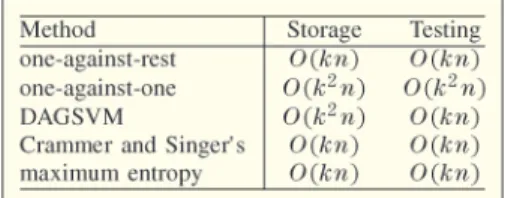
For linear classifiers, one-against-one method is shown to give better testing accuracy than one-against-rest method [57]. However, it requires Oðk2nÞspaces for storing models andOðk2nÞcost for testing an instance; both are more expensive than the one-against-rest method. Interestingly, for nonlinear classifiers via kernels, one-against-one method does not have such disadvantages [50]. DAGSVM [58] is the same as one-against-one
method but it attempts to reduce the testing cost. Starting with a candidate set of all classes, this method sequentially selects a pair of classes for prediction and removes one of the two. That is, if a binary classifier of classiandjpredictsi, thenjis removed from the candidate set. Alternatively, a prediction of class j will cause i to be removed. Finally, the only remained class is the predicted result. For any pairði;jÞconsidered, the true class may be neitherinorj. However, it does not matter which one is removed because all we need is that if the true class is involved in a binary prediction, it is the winner. Because classes are sequentially removed, onlyk1 models are used. The testing time complexity of DAGSVM is thusOðnkÞ. B. Considering All Data at Once
In contrast to using many binary models, some have proposed solving a single optimization problem for multi-class multi-classification [59]–[61]. Here we discuss details of Crammer and Singer’s approach [60]. Assume class labels are 1;. . .;k. They consider the following optimization problem: min w1;...;wk 1 2 Xk m¼1 kwmk22þCX l i¼1 CS fwmgkm¼1;xi;yi (33) where CS fwmgkm¼1;x;y max m6¼y max 0;1 ðwywmÞ Tx : (34)
The setting is like combining all binary models of the one-against-rest method. There arekweight vectorsw1;. . .;wk
for k classes. In the loss function (34), for each m,
maxð0;1 ðwyiwmÞ
Tx
iÞis similar to the L1 loss in (8)
for binary classification. Overall, we hope that the decision value ofxiby the modelwyiis at least one larger than the
values by other models. For testing, the decision function is also (32).
Early works of this method focus on the nonlinear (i.e., kernel) case [50], [60], [62]. A study for linear classifica-tion is in [63], which applies a coordinate descent method to solve the dual problem of (33). The idea is similar to the method in Section IV-D; however, at each step, a larger subproblem ofkvariables is solved. A nice property of this k-variable subproblem is that it has a closed-form solution. Experiments in [63] show that solving (33) gives slightly better accuracy than one-against-rest method, but the training time is competitive. This result is different from
the nonlinear case, where the longer training time than one-against-rest and one-against-one methods has made the approach of solving one single optimization problem less practical [50]. A careful implementation of the ap-proach in [63] is given in [7, App. E].
C. Maximum Entropy
Maximum entropy (ME) [64] is a generalization of logistic regression for multiclass problems6and a special case of conditional random fields [65] (see Section VIII-A). It is widely applied by NLP applications. We still assume class labels 1;. . .;kfor an easy comparison to (33) in our subsequent discussion. ME models the following condi-tional probability function of labelygiven datax:
PðyjxÞ exp wT yx Pk m¼1exp wTmx (35)
wherewm;8m are weight vectors like those in (32) and (33). This model is also called multinomial logistic regression.
ME minimizes the following regularized negative log-likelihood: min w1;...;wm 1 2 Xk m¼1 kwkk2þC Xl i¼1 ME fwmgkm¼1;xi;yi (36) where ME fwmgkm¼1;x;y logPðyjxÞ:
Clearly, (36) is similar to (33) andMEð Þcan be consid-ered as a loss function. If wT
yixiw
T
mxi;8m6¼yi, then
MEðfwmgkm¼1;xi;yiÞis close to zero (i.e., no loss). On the
other hand, if wT
yixi is smaller than other w
T
mxi, m6¼yi,
thenPðyijxiÞ 1 and the loss is large. For prediction, the
decision function is also (32).
NLP applications often consider a more general ME model by using a functionfðx;yÞto generate the feature vector PðyjxÞ exp w Tfðx;yÞ ð Þ P y0expðwTfðx;y0ÞÞ : (37)
Equation (35) is a special case of (37) by
fðxi;yÞ ¼ 0 .. . 0 xi 0 .. . 0 2 6 6 6 6 6 6 6 6 6 4 3 7 7 7 7 7 7 7 7 7 5 ) y1 2Rnk and w¼ w1 .. . wk 2 6 4 3 7 5: (38)
Many studies have investigated optimization methods for L2-regularized ME. For example, Malouf [66] com-pares iterative scaling methods [67], gradient descent, nonlinear conjugate gradient, and L-BFGS (quasi-Newton) method [68] to solve (36). Experiments show that quasi-Newton performs better. In [12], a framework is proposed to explain variants of iterative scaling methods [30], [67], [69] and make a connection to coordinate descent meth-ods. For L1-regularized ME, Andrew and Gao [40] propose an extension of L-BFGS.
Recently, instead of solving the primal problem (36), some works solve the dual problem. A detailed derivation of the dual ME is in [33, App. A.7]. Memisevic [70] pro-posed a two-level decomposition method. Similar to the coordinate descent method [63] for (33) in Section V-B, in [70], a subproblem of kvariables is considered at a time. However, the subproblem does not have a closed-form solution, so a second-level coordinate descent method is applied. Collinet al.[71] proposed an exponential gradient method to solve ME dual. They also decompose the prob-lem into k-variable subproblems, but only approximately solve each subproblem. The work in [33] follows [70] to apply a two-level coordinate descent method, but uses a different method in the second level to decide variables for update.
D. Comparison
We summarize storage (model size) and testing time of each method in Table 3. Clearly, one-against-one and DAGSVM methods are less practical because of the much higher storage, although the comparison in [57] indicates that one-against-one method gives slightly better testing accuracy. Note that the situation is very different for the 6
Details of the connection between logistic regression and maximum entropy can be found in, for example, [12, Sec. 5.2].
Table 3Comparison of Methods for Multiclass Linear Classification in Storage (Model Size) and Testing Time.nIs the Number of Features and kIs the Number of Classes
kernel case [50], where one-against-one and DAGSVM are very useful methods.
V I .
L I N E A R - C L A S S I F I C A T I O N
T E C H N I Q U E S F O R N O N L I N E A R
C L A S S I F I C A T I O N
Many recent developments of linear classification can be extended to handle nonstandard scenarios. Interestingly, most of them are related to training nonlinear classifiers. A. Training and Testing Explicit Data Mappings via Linear Classifiers
In some problems, training a linear classifier in the original feature space may not lead to competitive perfor-mances. For example, on ijcnn1 in Table 1, the testing accuracy (92.21%) of a linear classifier is inferior to 98. 69% of a nonlinear one with the RBF kernel. However, the higher accuracy comes with longer training and testing time. Taking the advantage of linear classifiers’ fast train-ing, some studies have proposed using the explicit nonlin-ear data mappings. That is, we considerðxiÞ,i¼1;. . .;l, as the new training set and employ a linear classifier. In some problems, this type of approaches may still enjoy fast training/testing, but achieve accuracy close to that of using highly nonlinear kernels.
Some early works, e.g., [72]–[74], have directly trained nonlinearly mapped data in their experiments. Changet al. [9] analyze when this approach leads to faster training and testing. Assume that the coordinate descent method in Section IV-D is used for training linear/kernelized classi-fiers7andðxÞ 2Rd. From Section IV-D, each coordinate
descent step takesOðdÞandOðnlÞoperations for linear and kernelized settings, respectively. Thus, ifdnl, the ap-proach of training explicit mappings may be faster than using kernels. In [9], the authors particularly study degree-2 polynomial mappings such as (5). The dimen-sionality isd¼Oðn2Þ, but for sparse data, theOðn2Þversus OðnlÞcomparison is changed toOðn2ÞversusOðnlÞ, where
nis the average number of nonzero values per instance. For large sparse data sets,nl, so their approach can be very efficient. Table 4 shows results of training/testing degree-2 polynomial mappings using three data sets in Table 1 with significant lower linear-SVM accuracy than RBF. We apply the same setting as [9, Sec. 4]. From Tables 1 and 4, we observed that training ðxiÞ;8iby a
linear classifier may give accuracy close to RBF kernel, but is faster in training/testing.
A general framework was proposed in [75] for various nonlinear mappings of data. They noticed that to perform the coordinate descent method in Section IV-D, one only needs thatuTðxÞin (27) andu uþyð
iiÞðxÞin
(28) can be performed. Thus, even if ðxÞ cannot be
explicitly represented, as long as these two operations can be performed, Algorithm 3 is applicable.
Studies in [76] and [77] designed linear classifiers to train explicit mappings of sequence data, where features correspond to subsequences. Using the relation between subsequences, they are able to design efficient training methods for very high-dimensional mappings.
B. Approximation of Kernel Methods via Linear Classification
Methods in Section VI-A train ðxiÞ;8iexplicitly, so they obtain the same model as a kernel method using Kðxi;xjÞ ¼ðxiÞTðxjÞ. However, they have limitations when the dimensionality of ðxÞis very high. To resolve the slow training/testing of kernel methods, approxima-tion is sometimes unavoidable. Among the many available methods to approximate the kernel, some of them lead to training a linear classifier. Following [78], we categorize these methods to the following two types.
• Kernel matrix approximation. This type of ap-proaches finds a low-rank matrix 2Rdl with
dl such thatT can approximate the kernel
matrixQ
Q¼T
Q: (39)
Assume ½x1;. . .;xl. If we replace Q in (16)
with Q, then (16) becomes the dual problem of training a linear SVM on the new set ðyi;xiÞ,
i¼1;. . .;l. Thus, optimization methods discussed in Section IV can be directly applied. An advantage of this approach is that we do not need to know an explicit mapping function corresponding to a kernel of our interest (see the other type of ap-proaches discussed below). However, this property causes a complicated testing procedure. That is, the approximation in (39) does not directly reveal how to adjust the decision function (3).
Early developments focused on finding a good approximation matrix . Some examples include Nystro¨m method [79], [80] and incomplete Cholesky factorization [81], [82]. Some works 7See the discussion in the end of Section IV-D about the connection
between Algorithm 3 and the popular decomposition methods for nonlinear SVMs.
Table 4Results of Training/Testing Degree-2 Polynomial Mappings by the Coordinate Descent Method in Section IV-D. The Degree-2 Polynomial Mapping Is Dynamically Computed During Training, Instead of Expanded Beforehand. The Last Column Shows the Accuracy Difference Between Degree-2 Polynomial Mappings and RBF SVM
(e.g., [19]) consider approximations other than (39), but also lead to linear classification problems. A recent study [78] addresses more on training and testing linear SVM after obtaining the low-rank approximation. In particular, details of the testing procedures can be found in [78, Sec. 2.4]. Note that linear SVM problems obtained after kernel approximations are often dense and have more instances than features. Thus, training algorithms suitable for such problems may be different from those for sparse document data. • Feature mapping approximation. This type of
ap-proaches finds a mapping function :Rn!Rd
such that
ðxÞTðtÞ Kðx;tÞ:
Then, linear classifiers can be applied to new data
ðx1Þ;. . .;ðxlÞ. The testing phase is straightfor-ward because the mappingð Þis available.
Many mappings have been proposed. Examples include random Fourier projection [83], random projections [84], [85], polynomial approximation [86], and hashing [87]–[90]. They differ in various aspects, which are beyond the scope of this paper. An issue related to the subsequent linear classifi-cation is that some methods (e.g., [83]) generate dense ðxÞ vectors, while others give sparse vectors (e.g., [85]). A recent study focusing on the linear classification after obtainingðxiÞ;8iis
in [91].
V I I .
T R A I N I N G L A R G E D A T A B E Y O N D
T H E M E M O R Y O R T H E D I S K C A P A C I T Y
Recall that we described some binary linear classification algorithms in Section IV. Those algorithms can work well under the assumption that the training set is stored in the computer memory. However, as the training size goes beyond the memory capacity, traditional algorithms may become very slow because of frequent disk access. Indeed, even if the memory is enough, loading data to memory may take more time than subsequent computation [92]. There-fore, the design of algorithms for data larger than memory is very different from that of traditional algorithms.If the data set is beyond the disk capacity of a single computer, then it must be stored distributively. Internet companies now routinely handle such large data sets in data centers. In such a situation, linear classification faces even more challenges because of expensive communica-tion cost between different computing nodes. In some recent works [93], [94], parallel SVM on distributed envi-ronments has been studied but they investigated only kernel SVM. The communication overhead is less serious
because of expensive kernel computation. For distributed linear classification, the research is still in its infancy. The current trend is to design algorithms so that computing nodes access data locally and the communication between nodes is minimized. The implementation is often con-ducted using distributed computing environments such as Hadoop [95]. In this section, we will discuss some ongoing research results.
Among the existing developments, some can be easily categorized as online methods. We describe them in Sec-tion VII-A. Batch methods are discussed in SecSec-tion VII-B, while other approaches are in Section VII-C.
A. Online Methods
An online method updates the modelwvia using some instances at a time rather than considering the whole training data. Therefore, not only can online methods handle data larger than memory, but also they are suitable for streaming data where each training instance is used only once. One popular online algorithm is the stochastic gradient descent (SGD) method, which can be traced back to stochastic approximation method [96], [97]. Take the primal L2-regularized L1-loss SVM in (7) as an example. At each step, a training instance xi is chosen and w is
updated by w wrS 1 2kwk 2 2þCmaxð0;1yiwTxiÞ (40)
whererS is a subgradient operator and is the learning
rate. Specifically, (40) becomes the following update rule:
If 1yiwTxi>0;
then w ð1ÞwþCyixi: (41)
The learning rateis gradually reduced along iterations. It is well known that SGD methods have slow con-vergence. However, they are suitable for large data because of accessing only one instance at a time. Early studies which have applied SGD to linear classification include, for example, [98] and [99]. For data with many features, recent studies [5], [26] show that SGD is effective. They allow more flexible settings such as using more than one training instance at a time. We briefly discuss the online setting ofPegasos[5]. In Algorithm 1, at each step a), a small random subset B is used instead of the full set. Similar convergence properties to that described in Section IV-B still hold but in expectation (see [5, Th. 2]). Instead of solving the primal problem, we can design an online algorithm to solve the dual problem [6], [100]. For example, the coordinate descent method in Algorithm 3 can be easily extended to an online setting by replacing the 2596
sequential selection of variables with a random selection. Notice that the update rule (28) is similar to (41), but has the advantage of not needing to decide the learning rate. This online setting falls into the general framework of randomized coordinate descent methods in [101] and [102]. Using the proof in [101], the linear convergence in expectation is obtained in [6, App. 7.5].
To improve the convergence of SGD, some [103], [104] have proposed using higher order information. The rule in (40) is replaced by
w wHrSð Þ (42)
where H is an approximation of the inverse Hessian r2fðwÞ1
. To save the cost at each update, practicallyHis a diagonal scaling matrix. Experiments [103] and [104] show that using (42) is faster than (40).
The update rule in (40) assumes L2 regularization. While SGD is applicable for other regularization, it may not perform as well because of not taking special pro-perties of the regularization term into consideration. For example, if L1 regularization is used, a standard SGD may face difficulties to generate a sparse w. To address this problem, recently several approaches have been proposed [105]–[110]. The stochastic coordinate descent method in [106] has been extended to a parallel version [111].
Unfortunately, most existing studies of online algo-rithms conduct experiments by assuming enough memory and reporting the number of times to access data. To apply them in a real scenario without sufficient memory, many practical issues must be checked.Vowpal-Wabbit[112] is one of the very few implementations which can handle data larger than memory. Because the same data may be accessed several times and the disk reading time is expen-sive, at the first pass, Vowpal-Wabbit stores data to a compressed cache file. This is similar to the compression strategy in [92], which will be discussed in Section VII-B. Currently,Vowpal-Wabbitsupports unregularized linear classification and regression. It is extended to solve L1-regularized problems in [105].
Recently,Vowpal-Wabbit(after version 6.0) has sup-ported distributed online learning using the Hadoop [95] framework. We are aware that other Internet companies have constructed online linear classifiers on distributed environments, although details have not been fully avail-able. One example is the system SETI at Google [113]. B. Batch Methods
In some situations, we still would like to consider the whole training set and solve a corresponding optimization problem. While this task is very challenging, some (e.g., [92] and [114]) have checked the situation that data are larger than memory but smaller than disk. Because of
ex-pensive disk input/output (I/O), they design algorithms by reading a continuous chunk of data at a time and mini-mizing the number of disk accesses. The method in [92] extends the coordinate descent method in Section IV-D for linear SVM. The major change is to update more variables at a time so that a block of data is used together. Specifically, in the beginning, the training set is randomly partitioned to m files B1;. . .;Bm. The available memory
space needs to be able to accommodate one block of data and the working space of a training algorithm. To solve (16), sequentially one block of data B is read and the following function ofd is minimized under the condition 0iþdiC; 8i2B and di¼0;8i62B fDðAþdÞ fDðAÞ ¼ 1 2d T BQBBdBþdTBðQAeÞB ¼ 1 2d T BQBBdBþ X i2B yidiðuTxiÞ dTBeB (43) whereQBBis a submatrix ofQanduis defined in (26). By
maintaining uin a way similar to (28), equation (43) in-volves only data in the block B, which can be stored in memory. Equation (43) can be minimized by any tradi-tional algorithm. Experiments in [92] demonstrate that they can train data 20 times larger than the memory capa-city. This method is extended in [115] to cache informative data points in the computer memory. That is, at each iteration, not only the selected block but also the cached points are used for updating corresponding variables. Their way to select informative points is inspired by the shrink-ing techniques used in trainshrink-ing nonlinear SVM [8], [47].
For distributed batch learning, all existing parallel optimization methods [116] can possibly be applied. How-ever, we have not seen many practical deployments for training large-scale data. Recently, Boydet al. [117] have considered the alternating direction method of multiplier (ADMM) [118] for distributed learning. Take SVM as an example and assume data points are partitioned to m dis-tributively stored setsB1;. . .;Bm. This method solves the
following approximation of the original optimization problem: min w1;...;wm;z 1 2z TzþCX m j¼1 X i2Bj L1ðwj;xi;yiÞ þ 2 Xm j¼1 kwjzk2 subject to wjz¼0;8j
where is a prespecific parameter. It then employs an optimization method of multipliers by alternatively minimizing the Lagrangian function over w1;. . .;wm,
minimizing the Lagrangian overz, and updating dual mul-tipliers. The minimization of Lagrangian overw1;. . .;wm
can be decomposed to m independent problems. Other steps do not involve data at all. Therefore, data points are locally accessed and the communication cost is kept minimum. Examples of using ADMM for distributed training include [119]. Some known problems of this approaches are first that the convergence rate is not very fast, and second that it is unclear how to choose param-eter .
Some works solve an optimization problem using parallel SGD. The data are stored in a distributed system, and each node only computes the subgradient correspond-ing to the data instances in the node. In [120], a delayed SGD is proposed. Instead of computing the subgradient of the current iterate wk, in delayed SGD, each node com-putes the subgradient of a previous iteratorwðkÞ, where
ðkÞ k. Delayed SGD is useful to reduce the synchro-nization delay because of communication overheads or uneven computational time at various nodes. Recent works [121], [122] show that delayed SGD is efficient when the number of nodes is large, and the delay is asymptotically negligible.
C. Other Approaches
We briefly discuss some other approaches which can-not be clearly categorized as batch or online methods.
The most straightforward method to handle large data is probably to randomly select a subset that can fit in memory. This approach works well if the data quality is good; however, sometimes using more data gives higher accuracy. To improve the performance of using only a subset, some have proposed techniques to include impor-tant data points into the subset. For example, the approach in [123] selects a subset by reading data from disk only once. For data in a distributed environment, subsampling can be a complicated operation. Moreover, a subset fitting the memory of one single computer may be too small to give good accuracy.
Bagging [124] is a popular classification method to split a learning task to several easier ones. It selects several random subsets, trains each of them, and ensembles (e.g., averaging) the results during testing. This method may be particularly useful for distributively stored data because we can directly consider data in each node as a subset. How-ever, if data quality in each node is not good (e.g., all instances with the same class label), the model generated by each node may be poor. Thus, ensuring data quality of each subset is a concern. Some studies have applied the bagging approach on a distributed system [125], [126]. For example, in the application of web advertising, Chakrabartiet al.[125] train a set of individual classifiers in a distributed way. Then, a final model is obtained by averaging the separate classifiers. In the linguistic appli-cations, McDonald et al. [127] extend the simple model average to the weighted average and achieve better
perfor-mance. An advantage of the bagging-like approach is the easy implementation using distributed computing techni-ques such as MapReduce [128].8
V I I I .
R E L A T E D T O P I C S
In this section, we discuss some other linear models. They are related to linear classification models discussed in earlier sections.
A. Structured Learning
In the discussion so far, we assumed that the labelyiis a
single value. For binary classification, it isþ1 or1, while for multiclass classification, it is one of thekclass labels. However, in some applications, the label may be a more sophisticated object. For example, in part-of-speech (POS) tagging applications, the training instances are sentences and the labels are sequences of POS tags of words. If there are l sentences, we can write the training instances as ðyi;xiÞ 2YniXni;8i¼1;. . .;l, wherexi is the ith
sen-tence,yiis a sequence of tags,Xis a set of unique words in the context,Y is a set of candidate tags for each word, and niis the number of words in theith sentence. Note that
we may not be able to split the problem to several independent ones by treating each value yij of yi as the
label, becauseyijnot only depends on the sentencexibut
also other tags ðyi1;. . .;yiðj1Þ;yiðjþ1Þ;. . .yiniÞ. To handle
these problems, we could use structured learning models like conditional random fields [65] and structured SVM [129], [130].
• Conditional random fields (CRFs).The CRF [65] is a linear structured model commonly used in NLP. Using notation mentioned above and a feature functionfðx;yÞlike ME, CRF solves the following problem: min w 1 2kwk 2 2þC Xl i¼1 CRFðw;xi;yiÞ (44) where CRFðw;xi;yiÞ logPðyijxiÞ PðyjxÞ exp w Tfðx;yÞ ð Þ P y0expðwTfðx;y0ÞÞ : (45)
If elements in yi are independent of each other, then CRF reduces to ME.
8
We mentioned earlier the Hadoop system, which includes a MapReduce implementation.
The optimization of (44) is challenging because in the probability model (45), the number of possible y’s is exponentially large. An important property to make CRF practical is that the gradient of the objective function in (44) can be efficiently evaluated by dynamic programming [65]. Some available optimization methods include L-BFGS (quasi-Newton) and conjugate gradient [131], SGD [132], stochastic quasi-Newton [103], [133], and trust region Newton method [134]. It is shown in [134] that the Hessian-vector product (23) of the Newton method can also be evaluated by dynamic programming.
• Structured SVM.Structured SVM solves the follow-ing optimization problem generalized form multi-class SVM in [59], [60]: min w 1 2kwk 2 2þC Xl i¼1 SSðw;xi;yiÞ (46) where SSðw;xi;yiÞ max y6¼yi max0;ðyi;yÞ wTðfðxi;yiÞ fðxi;yÞÞ
andð Þis a distance function withðyi;yiÞ ¼0 and ðyi;yjÞ ¼ðyj;yiÞ. Similar to the relation between conditional random fields and maximum entropy, if
ðyi;yjÞ ¼ 0; if yi¼yj 1; otherwise (
and yi2 f1;. . .;kg;8i, then structured SVM be-comes Crammer and Singer’s problem in (33) fol-lowing the definition offðx;yÞandwin (38).
Like CRF, the main difficulty to solve (46) is on handling an exponential number ofyvalues. Some works (e.g., [25], [129], and [135]) use a cutting plane method [136] to solve (46). In [137], a sto-chastic subgradient descent method is applied for both online and batch settings.
B. Regression
Given training data fðzi;xiÞgil¼1RRn, a regres-sion problem finds a weight vector w such that wTx
i
zi;8i. Like classification, a regression task solves a risk
minimization problem involving regularization and loss
terms. While L1 and L2 regularization is still used, loss functions are different, where two popular ones are
LSðw;x;zÞ 1 2ðzw
TxÞ2
(47)
ðw;x;zÞ max0;jzwTxj : (48)
The least square loss in (47) is widely used in many places, while the-insensitive loss in (48) is extended from the L1 loss in (8), where there is a user-specified parameteras the error tolerance. Problem (7) with L2 regularization and -insensitive loss is called support vector regression (SVR) [138]. Contrary to the success of linear classifica-tion, so far not many applications of linear regression on large sparse data have been reported. We believe that this topic has not been fully explored yet.
Regarding the minimization of (7), if L2 regulariza-tion is used, many optimizaregulariza-tion methods menregulariza-tioned in Section IV can be easily modified for linear regression.
We then particularly discuss L1-regularized least square regression, which has recently drawn much atten-tion for signal processing and image applicaatten-tions. This research area is so active that many optimization methods (e.g., [49] and [139]–[143]) have been proposed. However, as pointed out in [13], optimization methods most suitable for signal/image applications via L1-regularized regression may be very different from those in Section IV for classi-fying large sparse data. One reason is that data from signal/ image problems tend to be dense. Another is that xi;8i
may be not directly available in some signal/image prob-lems. Instead, we can only evaluate the product between the data matrix and a vector through certain operators. Thus, optimization methods that can take this property into their design may be more efficient.
I X .
C O N C L U S I O N
In this paper, we have comprehensively reviewed recent advances of large linear classification. For some applica-tions, linear classifiers can give comparable accuracy to nonlinear classifiers, but enjoy much faster training and testing speed. However, these results do not imply that nonlinear classifiers should no longer be considered. Both linear and nonlinear classifiers are useful under different circumstances.
Without mapping data to another space, for linear classification we can easily prepare, select, and manipulate features. We have clearly shown that linear classification is not limited to standard scenarios like document classifi-cation. It can be applied in many other places such as efficiently approximating nonlinear classifiers. We are confident that future research works will make linear classification a useful technique for more large-scale applications.h