The Discrete Particle Swarm Optimization Algorithms For Permutation Flowshop Scheduling Problem

(1)

https://doi.org/10.22219/JTIUMM.Vol20.No2.1-12 http://ejournal.umm.ac.id/index.php/industri [email protected]

Please cite this article as: Amallynda, I. (2019). The Discrete Particle Swarm Optimization Algorithms For Permutation Flowshop Scheduling Problem. Jurnal Teknik Industri, 20(2), 1-12. doi:https://doi.org/10.22219/JTIUMM.Vol20.No2.1-12

The Discrete Particle Swarm Optimization Algorithms For

Multi-Objective Permutation Flowshop Scheduling Problem

Ikhlasul Amallynda

Department of Industrial Engineering, University Of Muhammadiyah Malang Jl. Raya Tlogomas No. 246 Malang, Indonesia

Corresponding author: [email protected]

1. Introduction

The flow shop scheduling problem is one of the best-known production scheduling problems. It has been classified into an NP-complete problem. In the pure flow shop scheduling problem, there are n jobs processed on m machines in the same order, and the operation of every job must be processed on machine k. The Permutation Flow Shop Scheduling Problem (PFSP) is the case with the same job sequence in all machines. Permutation schedules do not always cover the optimal schedule except for the case of two machines [1]. PFSP assumed a Static and deterministic environment. The processing time and due date are known. Moreover, all job is available for processing from the beginning. Preemptions are not permitted when the job begins to be processed on a machine. It cannot be interrupted. One of the most relevant flow shop applications was found in the chemical industry.

The primary purpose of the schedule is finding the optimal Job sequence. It is seen from some performance criteria, such as makespan, total flowtime, and mean lateness.

ARTICLE INFO ABSTRACT

Article history

Received March 28, 2019 Revised July 10, 2019 Accepted August 20, 2019 Available Online August 31, 2019

In this paper, two types of discrete particle swarm optimization (DPSO) algorithms are presented to solve the Permutation Flow Shop Scheduling Problem (PFSP). We used criteria to minimize total earliness and total tardiness. The main contribution of this study is a new position update method is developed based on the discrete domain because PFSP is represented as discrete job permutations. In addition, this article also comes with a simple case study to ensure that both the proposed algorithm can solve the problem well in the short computational time. The result of Hybrid Discrete Particle Swarm Optimization (HDPSO) has a better performance than the Modified Particle Swarm Optimization (MPSO). The HDPSO produced the optimal solution. However, it has a slightly longer computation time. Besides the population size and maximum iteration have impact on the quality of solutions produced by HDPSO and MPSO algorithms.

This is an open-access article under the CC–BY-SA license.

Keywords Flow shop Earliness Tardiness Metaheuristic

(2)

Lateness measures the conformity of the schedule to a given due date. It has negative values whenever a job is completed early. Negative lateness represents earlier service than requested. Conversely, the positive lateness represents later service than requested job earliness may cause bounded capital and inventory holding costs. Furthermore, job

tardiness may disrupt a customer’s operations and incurring penalty fees. Therefore, both

earliness and tardiness should be taken into account in order to determine the optimal machine scheduling policy. The sequence of jobs affects performance measures. Multiple objective functions are possible that the objective function is not optimal when other objective functions are optimized. There is a trade-off when there are two objective functions simultaneously optimized. Therefore, It is a multi-objective problem.

Some exact and heuristic algorithms have been proposed over the past decades. These have been used for solving the PFSP with the objectives of minimizing total earliness and total tardiness. Scheduling problems with multiple performances is a combinatorial problem that classified into the NP-Hard problem. The best method to solve NP-Hard problem is heuristic [2]. Some research has used a metaheuristic method to solved PSFP problems for a single objective, and multi-objective problems. Some that metaheuristics such as Tabu Search (TS) [3-7], Genetic Algorithm (GA) [8-14], Simulated Annealing (SA) [15-17], Particle Swarm Optimization (PSO) [18-22]. However, there is a few research that considers minimizing the total earliness and total tardiness simultaneously in PFSP.

The PSO algorithm is an efficient algorithm for scheduling problems with various variations [23]. Originally, PSO has developed to solve continuous optimization problems. Scheduling is a discrete and combinatorial problem. This research modified PSO to solve the problem. In this paper, This research proposes two PSO-based algorithms to find the optimal sequence in PFSP. This research used criteria minimizing total earliness and total tardiness simultaneously. The modifications are carried out by changing the speed update formula and by using a transition probability matrix. For the multi-objective function, we used the multi-objective function by Ronconi & Birgin[24]. The main contribution of this paper is since a new position update method is developed to be applied to all classes of combinatorial optimization problems in the literature. The rest of the paper is organized as follows. Section 2 presents the assumption, mathematical model, proposed algorithm, case study, and parameter setting. In section 3, we describe results and discussion, and Section 4 is a conclusion and future work.

2. Methodology

We modified some algorithms based on Hybrid Discrete Particle Swarm Optimization (HDPSO) algorithm by Clerc[25] and modified particle swarm optimization (MPSO) algorithm by Santosa, Siswanto & Putawama [26] to solve the PFSP problem. We modified the HDPSO and MPSO the formulation to reach the global optimal point accurately and efficiently.

2.1 Assumption

Generally, the scheduling problem is divided into two types: flow shop and job shop scheduling. The flow shop scheduling attracts the researcher [27]. In the PFSP, a set of jobs (N = 1,2,3,...n) be processed through the set of machines M (M=1,2,3,...,m) in the same order. The processing times of the jobs at the machines are known, non-negative, and deterministic. Furthermore, some assumptions PFSP problems: 1) all jobs are independent and they ready to be processed at time 0; 2) The machine is always available and ready to use (no damage); 3) Each machine only process one job at a time; 4) Each job

(3)

only be processed on one machine at a time; 5) Any job that is being processed on one machine cannot be interrupted (no pre-emption); 6) Setup time is independent of the sequence and is included in the processing time; 7) Storage capacity between stages of operation (in process storage) is unlimited [2]. In scheduling, the possible sequence if there are n jobs is n!. in most literature, the search for solutions to this problem is Permutation Flow Shop Scheduling Problem (PFSP).

2.2 Mathematical Model

The mathematical model in this paper is the modification of Ronconi & Birgin [24]. The model was developed by adding and changing constraints. The objective functions are minimizing total earliness and total tardiness. Two objective functions have some weight, and It to be minimized simultaneously.

𝑖 : operation index 𝑗 : job index 𝑘 : machine index

𝑝𝑗𝑘 : processing time of job 𝑗 at machine 𝑘 𝑑𝑗 : due date of job 𝑗

𝑆𝑖𝑗 : starting time of job 𝑗 at operation 𝑖 𝐶𝑖𝑗 : completion time of job 𝑗 at operation 𝑖 𝐸𝑗 : earliness time of job 𝑗

𝑇𝑗 : tardiness time of job 𝑗

𝑥𝑖𝑗 : binary variable, 1 if job 𝑗 at operation 𝑖 and 0 if not

Min ∑𝑛𝑗=1𝐸𝑗+ 𝑇𝑗 (1) Constraint 𝑇𝑗≥ 𝐶𝑗𝑚− ∑𝑖=1𝑛 𝑥𝑖𝑗𝑑𝑖 j = 1, 2, ..., n (2) 𝐸𝑗 ≥ ∑𝑛𝑖=1𝑥𝑖𝑗𝑑𝑖− 𝐶𝑗𝑚 j = 1, 2, ..., n (3) 𝐶𝑗𝑚= 𝑆𝑗𝑚+ ∑𝑖=1𝑛 𝑥𝑖𝑗𝑝𝑖𝑚 j = 1, 2, ..., n (4) 𝑆𝑗+1,𝑘≥ 𝑆𝑗𝑘+ ∑𝑖=1𝑛 𝑥𝑖𝑗𝑝𝑖𝑘 j = 1, 2, ..., n-1, k = 1, 2, ..., m (5) 𝑆𝑗,𝑘+1≥ 𝑆𝑗𝑘+ ∑𝑛𝑖=1𝑥𝑖𝑗𝑝𝑖𝑘 j= 1, 2, …, n, k = 1, 2, …, m-1 (6) 𝑆11≥ 0 (7) ∑𝑛𝑖=1𝑥𝑖𝑗= 1 j = 1, 2, ..., n (8) ∑𝑛𝑗=1𝑥𝑖𝑗 = 1 j = 1, 2, ..., n (9) Equation (1) is the multi-objective function to minimize total earliness and total tardiness simultaneously. Constraint (2) show the formula tardiness of each job. Constraint (3) explain the individual earliness of each job. Equation (4) describe the completion time of each job on the last machine. Constraints (5) – (7) show the rules for the starting time of each job on each machine. Constraint (5) describes the starting times of consecutive jobs on a machine. Constraint (6) indicates the starting times of a job on two consecutive machines. Constraint (7) show the starting time of the first job on the first machine must be non-negative. Constraints (8) and (9) ensure that a job is allocated to a sequence position. These ensure each sequence position only one job.

2.3 Proposed Algorithm

PSO is an algorithm based on swarm intelligence. It was proposed J. Kennedy and R. C. Eberhart [28]. PSO has three main components, including particles, cognitive components, and social components, and particle velocity. Moreover, each particle represents a solution. in Cognitive learning, pBest is the best position by a particle.

(4)

Furthermore, gBest is the best position of the whole particle in the swarm. pBest is the best position of each particle among iterations. Moreover, gBest is the best of pBest. The disadvantage of PSO is the possibility of being trapped at local optimal. It is occurred to solve discrete optimization problems such as job scheduling. The modification by changing the updating mechanism can reduce the possibility of being trapped at local optimal. We developed two procedures. It is Hybrid Discrete Particle Swarm Optimization (HDPSO) and Modified Particle Swarm Optimization (MPSO).

2.3.1 Hybrid Discrete Particle Swarm Optimization (HDPSO)

Clerc [25] modified the Discrete Particle Swarm Optimization (DPSO) algorithm that was formulated by Kennedy and Eberhart. He modified the representation of the position of the particles, the shape of the velocity produced by the particles, and the effect of velocity on the position of the particles. The goal of these modifications is to be applied to problems with discrete models, especially types combinatorial. This research modified The structure of the DPSO algorithm by Clerc [25]:

1. Particles position

𝑥_𝑖𝑡 = [𝑥_𝑖1𝑡 𝑥_𝑖2𝑡 .. 𝑥_𝑖𝑑𝑡 ]

Where, 𝑥_𝑖𝑡_{is the position of the 𝑖}𝑡ℎ_{-particle in the 𝑡}𝑡ℎ_{-iteration and the particle have as} many as 𝑑 dimensions.

2. Transposition

Transposition is a way to exchange two values on a particular dimension based on the index sequence of the position of the particles.

3. Velocity

Velocity, as much as ‖𝑣_𝑖𝑡‖ Transposition process between the two index positions. Velocity is defined as follows:

𝑣𝑖𝑡= ((𝑎𝑘, 𝑏𝑘)), 𝑎 ∈ {1,2, … , 𝑑}, 𝑏 ∈ {1,2, … , 𝑑}, 𝑘 ↑1 ‖𝑣_𝑖𝑡‖

‖𝑣_𝑖𝑡‖ is the number of lists of transpositions, 𝑎 and 𝑏 are the dimensional dimension indices that be exchanged for value. For example: 𝑣1= ((1,3), (2,5)) and 𝑣2 = ((2,5), (1,3)), then 𝑣1 @ 𝑣2 said to be not the same; however both are congruent.

4. Opposite of velocity

Based on point (3) above, it can be said that 𝑣1 is opposite of 𝑣2, that is 𝑣1= ¬𝑣2 moreover, can be written 𝑣₂= ¬𝑣1. Therefore that the general form applies that ¬¬𝑣 = 𝑣 and 𝑣 ⨁ ¬𝑣 ≅ ∅. If 𝑣_𝑖𝑡_{= ((𝑎} 𝑘, 𝑏𝑘)), 𝑘 ↑1 ‖𝑣𝑖𝑡‖_{, then ¬𝑣} 𝑖𝑡 = ((𝑎𝑘, 𝑏𝑘)), 𝑘 ↓1 ‖𝑣𝑖𝑡‖_{= ((𝑎} ‖𝑣_𝑖𝑡‖−𝑘+1, 𝑏‖𝑣_𝑖𝑡‖−𝑘+1)) , 𝑘 ↑1 ‖𝑣𝑖𝑡‖ Example: 𝑣𝑖𝑡= ((1,3), (3,2), (4,5)) → 𝑣𝑖𝑡= ((𝑎1, 𝑏1), (𝑎2, 𝑏2), (𝑎3, 𝑏3)), ‖𝑣𝑖𝑡‖ = 3 ¬𝑣_𝑖𝑡 = ((4,5), (3,2), (1,3)) ¬¬𝑣_𝑖𝑡 = ((1,3), (3,2), (4,5)) 5. Move “position plus velocity.”

Suppose the position update, 𝑥_𝑖𝑡+1 _{= 𝑥}

𝑖𝑡+ 𝑣𝑖𝑡+1 is operated by processing from the first sequence of transposition 𝑣 to position 𝑥, then the next sequence, until the final sequence of 𝑣.

For example:

𝑥10= [2 5 1 3 4] → 𝑥𝑖𝑡 = [𝑥𝑖1𝑡 𝑥𝑖2𝑡 .. 𝑥𝑖𝑑𝑡 ]

𝑣10= ((1,3), (3,2), (4,5)) → 𝑣𝑖𝑡 = ((𝑎1, 𝑏1), (𝑎2, 𝑏2), (𝑎3, 𝑏3)), ‖𝑣𝑖𝑡‖ = 3 𝑥_𝑖𝑡+1 = 𝑥_𝑖𝑡+ 𝑣_𝑖𝑡+1

(5)

Please cite this article as: Amallynda, I. (2019). The Discrete Particle Swarm Optimization Algorithms For Permutation Flowshop Scheduling Problem. Jurnal Teknik Industri, 20(2), 1-12. doi:https://doi.org/10.22219/JTIUMM.Vol20.No2.1-12 𝑥11= 𝑥10+ 𝑣11 𝑥11= [2 5 1 3 4] + ((1,3), (3,2), (4,5)) 𝑥11= [1 5 2 3 4] + ((3,2), (4,5)) 𝑥11= [1 2 5 3 4] + ((4,5)) 𝑥11= [1 2 5 4 3]

6. Subtraction “position minus position.”

For example, there are two positions 𝑥_𝑖𝑡_{and 𝑥}

𝑖𝑡+1. Subtraction 𝑥𝑖𝑡+1− 𝑥𝑖𝑡 is defined as a velocity of 𝑣_𝑖𝑡+1_{. Therefore that by applying the velocity}_𝑣

𝑖𝑡+1 into position 𝑥𝑖𝑡 produce 𝑥_𝑖𝑡+1. The difference is defined as follows:

𝑥_𝑖𝑡+1− 𝑥_𝑖𝑡 = 𝑣_𝑖𝑡+1↔ 𝑥_𝑖𝑡+ 𝑣_𝑖𝑡+1 = 𝑥_𝑖𝑡+1

if 𝑥_𝑖𝑡+1 = 𝑥_𝑖𝑡, then 𝑥_𝑖𝑡+1− 𝑥_𝑖𝑡 = 𝑣_𝑖𝑡+1= ∅. For example: 𝑥11= [1 2 5 4 3] and 𝑥10= [2 5 1 3 4] 𝑣11= 𝑥11− 𝑥10 = ((1,3), (3,2), (4,5))

7. Addition “velocity plus velocity.”

Suppose there are two speeds 𝑣1 and 𝑣2, to increase the speed of 𝑣1 with 𝑣2 (𝑣1 ⨁ 𝑣2), the addition operation is carried out using the transposition sequence 𝑣₁ then proceed with the transposition sequence 𝑣2. Besides that, it can be defined as follows:

𝑣 = 𝑣1 ⨁ 𝑣2 𝑣 = ((𝑎1, 𝑏1), (𝑎2, 𝑏2), … , (𝑎‖𝑣1‖, 𝑏‖𝑣1‖)₁) ⨁ ((𝑎1, 𝑏1), (𝑎2, 𝑏2), … , (𝑎‖𝑣2‖, 𝑏‖𝑣2‖)₂) Example: 𝑣1= ((1,3), (3,2), (4,5)) 𝑣2= ((3,4), (4,1)) 𝑣 = 𝑣1 ⨁ 𝑣2= ((1,3), (3,2), (4,5)) ⨁ ((3,4), (4,1)) 𝑣 = ((1,3), (3,2), (4,5), (3,4), (4,1))

8. Multiplication “coefficient times velocity.”

Suppose that 𝑐 is a coefficient and (𝑐 ∈ R), then the multiplication between velocity 𝑣 and 𝑐 can be carried out as follows according to the condition of the coefficient value. a. If 𝑐 = 0, then 𝑣′_{= 𝑐. 𝑣} 𝑣′‖ = 𝑐. ‖𝑣‖ 𝑣′_{‖ = 0. ‖𝑣‖} 𝑣′_{‖ = 0} 𝑣′= ∅

b. If 0 < 𝑐 ≤ 1, 𝑣 cut to length: 𝑣′‖ = ⌈𝑐. ‖𝑣‖⌉. For example: 𝑣 = ((1,3), (3,2), (4,5))

‖𝑣‖ = 3 𝑣′= 𝑐. 𝑣

𝑣′_{‖ = ⌈0.1 ∗ 3⌉ = ⌈0.3⌉ = 1} 𝑣′= ((1,3))

c. If 𝑐 > 1, then 𝑐 is formed from 𝑐 = 𝑘 + 𝑐′_{which is 𝑘 = ⌊𝑐⌋, 𝑘 ∈ (𝑁 > 0), 𝑐}′ _{= 𝑐 − 𝑘 dan} 0 < 𝑐′_{< 1. So this case is defined as:}

𝑣′= (∑ 𝑣 𝑘

1

) ⨁ (𝑐′∗ 𝑣) = 𝑣 ⨁ v ⨁ … ⨁ v ⨁ (𝑐′∗ 𝑣) (𝑐′. 𝑣) is calculated using conditions (b).

Example:

𝑣 = ((1,3), (3,2), (4,5)) ‖𝑣‖ = 3

(6)

𝑘 = ⌊𝑐⌋ = ⌊2,5⌋ = 2 and 𝑐′ = 𝑐 − 𝑘 = 2,5 − 2 = 0,5

‖𝑣′_{‖ = ‖𝑣‖ + ‖𝑣‖ + (⌈𝑐}′_{∗ ‖𝑣‖⌉) = 3 + 3 + ⌈0,5 ∗ 3⌉ = 3 + 3 + ⌈1,5⌉} ‖𝑣′_{‖ = 3 + 3 + 2 = 8}

𝑣′= ((1,3), (3,2), (4,5)(1,3), (3,2), (4,5)(1,3), (3,2))

d. If 𝑐 < 1, then the velocity is reversed (𝑣 = ¬𝑣) using the concept on slide 8 and the value 𝑐 be positive 𝑐 = |𝑐|. Therefore that the latest velocity can be operated using the following function.

𝑣′= 𝑐. ¬𝑣, Where the value of 𝑐 be operated as in condition (a), (b), and (c) in the previous slide. For example:

𝑣′= 𝑐. ¬𝑣

𝑣′_{‖ = ⌈𝑐}′_{∗ ‖¬𝑣‖⌉ = ⌈0,1 ∗ 3⌉ = ⌈0,3⌉ = 1} 𝑣′_{= ((4,5))}

9. Distance between two position

The distance between the two particles is obtained by calculating the difference in the fitness value of the two positions.

10. The position update formula that has been modified is defined as follows: 𝑣𝑖𝑡+1= 𝑐1. 𝑣𝑖𝑡 ⨁ 𝑐2((𝑝𝐵𝑒𝑠𝑡𝑖𝑡+ 1 2(𝑔𝐵𝑒𝑠𝑡𝑔 𝑡 _{− 𝑝𝐵𝑒𝑠𝑡} 𝑖𝑡)) − 𝑥𝑖𝑡) (10) 𝑥𝑖𝑡+1 = 𝑥𝑖𝑡+ 𝑣𝑖𝑡+1 (11)

However, in its implementation, it was found that the PSO's particle speed was updated too quickly, and the minimum objective function value sought was often overlooked. Therefore, in this study, we changed the position update representation Clerc [25] by using the speed update formula developed by Shi and Eberhart [29]. The change of representation is carried out in the hope that particles are better in the process of approaching the optimal solution and not rapidly converging (early convergence). 𝑣_𝑖𝑗𝑡+1= 𝜃. 𝑣_𝑖𝑗𝑡 + 𝑐1𝑟1(𝑃𝑏𝑒𝑠𝑡𝑖𝑗𝑡 − 𝑥𝑖𝑗𝑡) + 𝑐2𝑟2(𝐺𝑏𝑒𝑠𝑡𝑔𝑗𝑡 − 𝑥𝑖𝑗𝑡) (12)

𝑥_𝑖𝑗𝑡+1 = 𝑥_𝑖𝑗𝑡 + 𝑣_𝑖𝑗𝑡+1 (13)

Equation (10) is the result of improvements that have been made, by adding an inertia

term (𝜃) to reduce the speed of the speed update formula. Usually the value of 𝜃 is made so that the higher the iteration is passed, the smaller the particle speed be. This value varies linearly in the range 0.9 to 0.4.

The weight of this inertia is proposed by Shi and Eberhart [29] to reduce speed during iterations, which allows the birds to converge the target points more accurately and efficiently. High inertia weight values add to the portion of the global exploration process, while low values emphasize local search. To not focus too much on one part and keep looking for a new search area in a particular dimension space, it is necessary to look for the inertial weight 𝜃 which equals keeping global and local searches. To achieve that and speed up convergence, an inertial weight that decreases in value by increasing iterations is used with the formula:

𝜃𝑡 = 𝜃𝑚𝑎𝑥− (

𝜃𝑚𝑎𝑥−𝜃𝑚𝑖𝑛

𝑖𝑚𝑎𝑥 ) 𝑖 (14)

where 𝜃𝑚𝑎𝑥 and 𝜃𝑚𝑖𝑛 are the initial and final inertia values, 𝑖𝑚𝑎𝑥 is the maximum number of iterations used, and 𝑖 is the current iteration.

11. Stopping criteria is the number of maximum iteration.

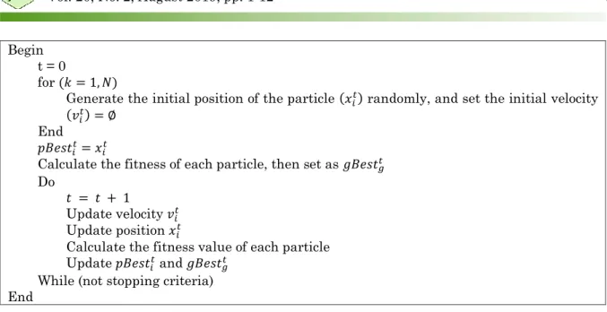
The pseudocode of the DPSO algorithm for the flow shop scheduling problem is presented in Fig. 1.

(7)

Begin t = 0

for (𝑘 = 1, 𝑁)

Generate the initial position of the particle (𝑥_𝑖𝑡₎_{randomly, and set the initial velocity}

(𝑣_𝑖𝑡_{) = ∅} End

𝑝𝐵𝑒𝑠𝑡_𝑖𝑡_{= 𝑥} 𝑖 𝑡

Calculate the fitness of each particle, then set as 𝑔𝐵𝑒𝑠𝑡𝑔𝑡 Do

𝑡 = 𝑡 + 1

Update velocity 𝑣_𝑖𝑡 Update position 𝑥_𝑖𝑡

Calculate the fitness value of each particle Update 𝑝𝐵𝑒𝑠𝑡_𝑖𝑡_and_{𝑔𝐵𝑒𝑠𝑡}

𝑔𝑡 While (not stopping criteria) End

Fig. 1. The proposed HDPSO algorithm structure 2.3.2 Modified Particle Swarm Optimization (MPSO)

The second proposed algorithm is a combination of the PSO algorithm with the probability transition matrix. This algorithm is called Modified Particle Swarm Optimization (MPSO) [26]. In this study, we modified the MPSO algorithm to solve the PFSP. The proposed algorithm be explained as follows.

1. Particles position 𝑥_𝑖𝑡 = [𝑥_𝑖1𝑡 𝑥_𝑖2𝑡 .. 𝑥_𝑖𝑑𝑡 ]

Where, 𝑥_𝑖𝑡_{is the position of the 𝑖}𝑡ℎ_{-particle in the 𝑡}𝑡ℎ_{-iteration, and the particle has as} many as 𝑑 dimensions. It is expressed in a probability transition matrix that is randomly generated with intervals of 0 to 1.

Example:

𝑥_𝑖𝑡 = [0.1067 0.8687 0.4314 0.1361 0.8530] 2. Solution sequence

The solution sequence is generated based on the probability value of the transition matrix. Normalize first the probability transition matrix such that the probability value is more than equal to 0 and less than 1.

Example:

If 𝑥𝑖𝑡 = [0.7749 1.2599 0.2638 0.5499 − 0.5132], it be normalized to

𝑥_𝑖𝑡 _{= [0.7749 1 0.2638 0.5499 0] moreover, be transposed to be a new solution.} 3. Transposition

Transposition is a way to exchange values on a particular dimension based on the index sequence of the position of the particles (by ascending or descending order).

Example:

a. Transposition by ascending order

𝑥_𝑖𝑡 = [0.1067 0.8687 0.4314 0.1361 0.8530] → 𝑠_𝑖𝑡 = [1 5 3 2 4] b. Transposition by descending order

𝑥𝑖𝑡 = [0.7749 1 0.2638 0.5499 0] → 𝑠𝑖𝑡 = [2 1 4 3 5] 4. Distance between two position

The distance between the two particles is obtained by calculating the difference in the fitness value of the two positions.

(8)

6. Stopping criteria is the number of maximum iteration (itmax).

The pseudocode of the MPSO algorithm for the flow shop scheduling problem is presented in Fig. 2.

Begin t = 0

for (𝑘 = 1, 𝑁)

Generate the probability transition matrix (𝑥_𝑖𝑡₎_{randomly [0,1], and set as the initial} position of the particles

Determine the initial solution based on the probability transition matrix, by sorting the probability values of each particle in ascending or descending order.

Set an initial velocity (𝑣_𝑖𝑡_{) = 0} End

𝑝𝐵𝑒𝑠𝑡_𝑖𝑡= 𝑥_𝑖𝑡

Calculate the fitness of each particle, then set as 𝑔𝐵𝑒𝑠𝑡𝑔𝑡 Do

𝑡 = 𝑡 + 1

Update velocity 𝑣_𝑖𝑡 Update position 𝑥_𝑖𝑡

Normalize the updated position and determine the new solution Calculate the fitness value of each particle

Update 𝑝𝐵𝑒𝑠𝑡_𝑖𝑡_and_{𝑔𝐵𝑒𝑠𝑡} 𝑔𝑡 While (not stopping criteria) End

Fig. 2. The proposed MPSO algorithm structure 2.4. The Case Study

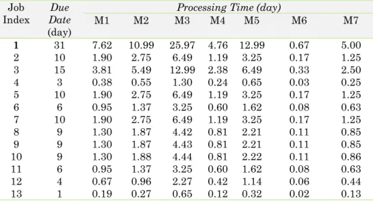
In this study, a case study was appointed by a cigarette company. The company produces a product if receives orders from the customer. The company used first come first served (FCFS) scheduling policy. It causes frequent delays in fulfilling order due dates. There are two types of lateness [1], such as tardiness and earliness. Each job must be processed in seven stages (machines) in the same order. The Job index, processing time and due date are shown in Table 1.

Table 1. The Job index, processing time and due date Job

Index DateDue

(day)

Processing Time (day)

M1 M2 M3 M4 M5 M6 M7 1 31 7.62 10.99 25.97 4.76 12.99 0.67 5.00 2 10 1.90 2.75 6.49 1.19 3.25 0.17 1.25 3 15 3.81 5.49 12.99 2.38 6.49 0.33 2.50 4 3 0.38 0.55 1.30 0.24 0.65 0.03 0.25 5 10 1.90 2.75 6.49 1.19 3.25 0.17 1.25 6 6 0.95 1.37 3.25 0.60 1.62 0.08 0.63 7 10 1.90 2.75 6.49 1.19 3.25 0.17 1.25 8 9 1.30 1.87 4.42 0.81 2.21 0.11 0.85 9 9 1.30 1.87 4.43 0.81 2.21 0.11 0.85 10 9 1.30 1.88 4.44 0.81 2.22 0.11 0.86 11 6 0.95 1.37 3.25 0.60 1.62 0.08 0.63 12 4 0.67 0.96 2.27 0.42 1.14 0.06 0.44 13 1 0.19 0.27 0.65 0.12 0.32 0.02 0.13

(9)

2.5 Parameter Setting

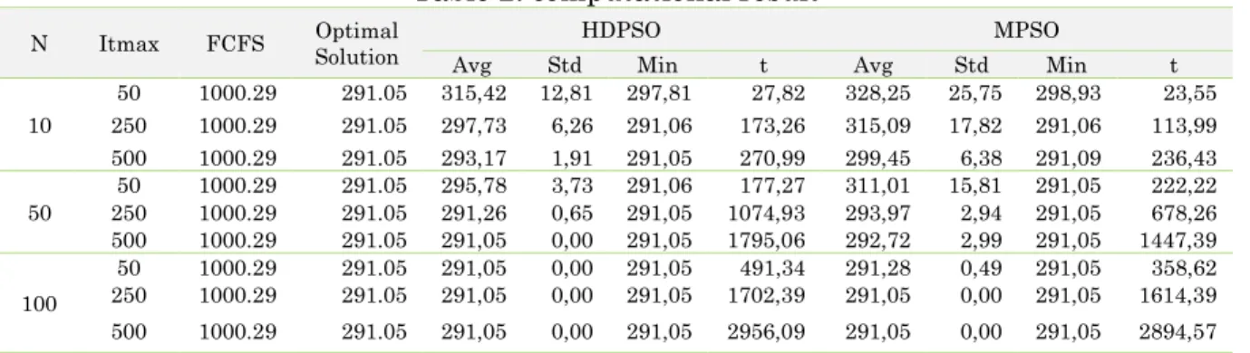
In experimental, We used some scenarios in the combination of tests. It consists of 9 combinations parameters consisting of: population size (N) and the maximum number of iterations (itmax). Population used 10, 50, 100, Iteration used 50, 250, 500. In addition, we set the other PSO parameters such as a) learning factor (𝑐₁ = 𝑐2= 1); b) inertia term (𝜃_𝑚𝑖𝑛 = 0,4 and 𝜃𝑚𝑎𝑥= 0,9) [30]. Each combination of parameters was tested for 10 replications. The computational process was carried out with the help of Matlab R2017a

software. It carried out on computers Intel® Core ™ i3-6006U CPU Processor @ 2.00GHz (4 CPUs). To evaluate the performance of HDPSO and MPSO algorithms, a paired t-test was carried out at the 95% significance level. [30]. On the other hand, the population and iteration effect on the solution's quality and computational time. The Test was conducted by the analysis of variance (ANOVA).

3 Results And Discussion

In this section, we compare the FCFS and the proposed algorithm. The computational test was carried out using 9 combinations of PSO algorithm parameters. The evaluation results are presented in Table 2.

Table 2. computational result

N Itmax FCFS _SolutionOptimal HDPSO MPSO

Avg Std Min t Avg Std Min t

10 50 1000.29 291.05 315,42 12,81 297,81 27,82 328,25 25,75 298,93 23,55 250 1000.29 291.05 297,73 6,26 291,06 173,26 315,09 17,82 291,06 113,99 500 1000.29 291.05 293,17 1,91 291,05 270,99 299,45 6,38 291,09 236,43 50 50 1000.29 291.05 295,78 3,73 291,06 177,27 311,01 15,81 291,05 222,22 250 1000.29 291.05 291,26 0,65 291,05 1074,93 293,97 2,94 291,05 678,26 500 1000.29 291.05 291,05 0,00 291,05 1795,06 292,72 2,99 291,05 1447,39 100 50 1000.29 291.05 291,05 0,00 291,05 491,34 291,28 0,49 291,05 358,62 250 1000.29 291.05 291,05 0,00 291,05 1702,39 291,05 0,00 291,05 1614,39 500 1000.29 291.05 291,05 0,00 291,05 2956,09 291,05 0,00 291,05 2894,57

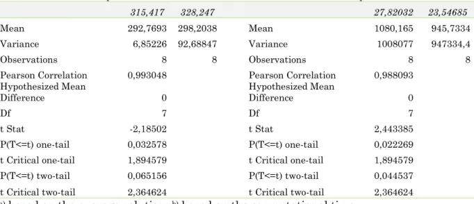
Based on the computation test in Table 2, the proposed algorithms produce better solutions than the company's solution. The proposed algorithm gave an optimal solution in a short time. In addition, the HDPSO algorithm has a better performance than the MPSO algorithm. However, HDPSO has a slightly longer computation time. Based on the paired t-test result (Table 3), the null hypothesis was rejected. It shows the difference between the HDPSO and MPSO algorithms. HDPSO produced better results than MPSO. However, HDPSO was computationally longer than MPSO.

Table 4 shows the ANOVA results. The population size (N) and maximum iteration (itmax) influence the quality of solutions HDPSO and MPSO algorithms. The alternative is that interaction does exist between the two factors. The ANOVA table shows a p-value of 0,003812 for HDPSO and 1,91E-09 for MPSO, which is smaller than α = 0.05. It

indicates that there are differences in the quality of solutions produced between the various population size categories and iteration.

(10)

Table 3. paired t-test results for proposed algorithms

a)_{t-Test: Paired Two Sample for Means} b)_{t-Test: Paired Two Sample for Means}

315,417 328,247 27,82032 23,54685

Mean 292,7693 298,2038 _Mean 1080,165 945,7334

Variance 6,85226 92,68847 _Variance 1008077 947334,4

Observations 8 8 _Observations 8 8

Pearson Correlation 0,993048 Pearson Correlation 0,988093 Hypothesized Mean

Difference 0 Hypothesized Mean Difference 0

Df 7 Df 7

t Stat -2,18502 t Stat 2,443385

P(T<=t) one-tail 0,032578 P(T<=t) one-tail 0,022269 t Critical one-tail 1,894579 t Critical one-tail 1,894579 P(T<=t) two-tail 0,065156 P(T<=t) two-tail 0,044537

t Critical two-tail 2,364624 t Critical two-tail 2,364624 a)_{based on the average solution;}b)_{based on the computational time}

Table 4. Two-factor ANOVA result for proposed algorithms

a)_{ANOVA (HDPSO test)}

Source of Variation SS df MS F P-value F crit

Sample 8267,508 2 4133,754 28,85902 3,45E-10 3,109311 Columns 3833,363 2 1916,682 13,38095 9,52E-06 3,109311 Interaction 2410,405 4 602,6011 4,206946 0,003812 2,484441

Within 11602,41 81 143,2396

Total 26113,68 89

b) _{ANOVA (MPSO test)}

Source of Variation SS df MS F P-value F crit

Sample 2134,902 2 1067,451 43,41859 1,53E-13 3,109311 Columns 1381,738 2 690,8688 28,1011 5,38E-10 3,109311 Interaction 1522,312 4 380,5781 15,48002 1,91E-09 2,484441 Within 1991,395 81 24,58512 Total 7030,347 89 5. Conclusion

The computational results show the proposed algorithms were successfully to solve the PFSP. It produces an optimal solution in the total earliness and total tardiness criterion. HDPSO produced better results than MPSO. However, HDPSO was computationally longer than MPSO. As future work, the proposed algorithms can be applied to the larger classes of combinatorial optimization problems in the literature and can be compared with other intelligent swarm algorithms.

References

[1] Y.-D. Kim, "Minimizing total tardiness in permutation flowshops," European

Journal of Operational Research, vol. 85, pp. 541-555, 1995.

(11)

[2] M. Avriel, M. Penn, and N. J. D. A. M. Shpirer, "Container ship stowage problem: complexity and connection to the coloring of circle graphs," vol. 103, pp. 271-279, 2000. https://doi.org/10.1016/S0166-218X(99)00245-0.

[3] V. A. Armentano and J. E. J. J. o. H. Claudio, "An application of a multi-objective tabu search algorithm to a bicriteria flowshop problem," vol. 10, pp. 463-481, 2004. https://doi.org/10.1023/B:HEUR.0000045320.79875.e3.

[4] J.-S. Chen, J. C.-H. Pan, and C.-K. J. E. S. w. A. Wu, "Hybrid tabu search for re-entrant permutation flow-shop scheduling problem," vol. 34, pp. 1924-1930, 2008. https://doi.org/10.1016/j.eswa.2007.02.027.

[5] B. Ekşioğlu, S. D. Ekşioğlu, P. J. C. Jain, and I. Engineering, "A tabu search

algorithm for the flowshop scheduling problem with changing neighborhoods," vol. 54, pp. 1-11, 2008. https://doi.org/10.1016/j.cie.2007.04.004.

[6] F. S. Erenay, I. Sabuncuoglu, A. Toptal, and M. K. J. E. J. o. O. R. Tiwari, "New solution methods for single machine bicriteria scheduling problem: Minimization of average flowtime and number of tardy jobs," vol. 201, pp. 89-98, 2010. https://doi.org/10.1016/j.ejor.2009.02.014.

[7] Y. Marinakis, M. J. C. Marinaki, and O. Research, "A hybrid multi-swarm particle swarm optimization algorithm for the probabilistic traveling salesman problem," vol. 37, pp. 432-442, 2010. https://doi.org/10.1016/j.cor.2009.03.004.

[8] C.-W. Chiou, W.-M. Chen, C.-M. Liu, and M.-C. J. E. S. w. A. Wu, "A genetic algorithm for scheduling dual flow shops," vol. 39, pp. 1306-1314, 2012. https://doi.org/10.1016/j.eswa.2011.08.008.

[9] W.-H. Wu, W.-H. Wu, J.-C. Chen, W.-C. Lin, J. Wu, and C.-C. J. J. o. M. S. Wu, "A heuristic-based genetic algorithm for the two-machine flowshop scheduling with learning consideration," vol. 35, pp. 223-233, 2015. https://doi.org/10.1016/j.jmsy.2015.02.002.

[10] N. Karimi, H. J. C. Davoudpour, and O. Research, "A high performing metaheuristic for multi-objective flowshop scheduling problem," vol. 52, pp. 149-156, 2014. https://doi.org/10.1016/j.cor.2014.01.006.

[11] H. F. Rahman, R. Sarker, and D. J. A. E. Essam, "A genetic algorithm for permutation flowshop scheduling under practical make-to-order production system," vol. 31, pp. 87-103, 2017. https://doi.org/10.1017/S0890060416000196. [12] S. A. Basir, M. M. Mazdeh, M. J. C. Namakshenas, and I. Engineering, "Bi-level

genetic algorithms for a two-stage assembly flow-shop scheduling problem with batch delivery system," vol. 126, pp. 217-231, 2018. https://doi.org/10.1016/j.cie.2018.09.035.

[13] C. Yu, Q. Semeraro, A. J. C. Matta, and O. Research, "A genetic algorithm for the hybrid flow shop scheduling with unrelated machines and machine eligibility," vol. 100, pp. 211-229, 2018. https://doi.org/10.1016/j.cor.2018.07.025.

[14] X. Liu, L. Wang, L. Kong, F. Li, and J. J. P. C. Li, "A Hybrid Genetic Algorithm for Minimizing Energy Consumption in Flow Shops Considering Ultra-low Idle State," vol. 80, pp. 192-196, 2019. https://doi.org/10.1016/j.procir.2018.12.013.

[15] T. Varadharajan and C. J. E. J. o. O. R. Rajendran, "A multi-objective simulated-annealing algorithm for scheduling in flowshops to minimize the makespan and total flowtime of jobs," vol. 167, pp. 772-795, 2005. https://doi.org/10.1016/j.ejor.2004.07.020.

[16] M. Bank, S. F. Ghomi, F. Jolai, and J. J. A. i. E. S. Behnamian, "Application of particle swarm optimization and simulated annealing algorithms in flow shop scheduling problem under linear deterioration," vol. 47, pp. 1-6, 2012. https://doi.org/10.1016/j.advengsoft.2011.12.001.

(12)

[17] P. Jarosław, S. Czesław, and Ż. J. P. C. S. Dominik, "Optimizing bicriteria flow

shop scheduling problem by simulated annealing algorithm," vol. 18, pp. 936-945, 2013. https://doi.org/10.1016/j.procs.2013.05.259.

[18] C.-J. Liao, C.-T. Tseng, P. J. C. Luarn, and O. Research, "A discrete version of particle swarm optimization for flowshop scheduling problems," vol. 34, pp. 3099-3111, 2007. https://doi.org/10.1016/j.cor.2005.11.017.

[19] S. Ponnambalam, N. Jawahar, and S. Chandrasekaran, "Discrete particle swarm optimization algorithm for flowshop scheduling," in Particle Swarm Optimization, ed: IntechOpen, 2009. https://www.intechopen.com/download/pdf/6275.

[20] F. P. Goksal, I. Karaoglan, F. J. C. Altiparmak, and I. Engineering, "A hybrid discrete particle swarm optimization for vehicle routing problem with simultaneous pickup and delivery," vol. 65, pp. 39-53, 2013. https://doi.org/10.1016/j.cie.2012.01.005.

[21] X. Zheng, S. Zhou, and H. J. I. J. o. P. R. Chen, "Ant colony optimisation algorithms for two-stage permutation flow shop with batch processing machines and nonidentical job sizes," vol. 57, pp. 3060-3079, 2019. https://doi.org/10.1080/00207543.2018.1529445.

[22] S. Sheikh, G. Komaki, V. J. C. Kayvanfar, and I. Engineering, "Multi objective two-stage assembly flow shop with release time," vol. 124, pp. 276-292, 2018. https://doi.org/10.1016/j.cie.2018.07.023.

[23] B. Jarraya and A. J. I. J. o. C. B. S. Bouri, "Metaheuristic optimization backgrounds: a literature review," vol. 3, 2012. https://ssrn.com/abstract=2114335. [24] D. P. Ronconi and E. G. Birgin, "Mixed-integer programming models for flowshop scheduling problems minimizing the total earliness and tardiness," in Just-in-Time

systems, ed: Springer, 2012, pp. 91-105.

https://doi.org/10.1007/978-1-4614-1123-9_5.

[25] M. Clerc, "Discrete particle swarm optimization, illustrated by the traveling salesman problem," in New optimization techniques in engineering, ed: Springer, 2004, pp. 219-239. https://doi.org/10.1007/978-3-540-39930-8_8.

[26] B. Santosa and N. Siswanto, "Discrete particle swarm optimization to solve multi-objective limited-wait hybrid flow shop scheduling problem," in IOP Conference

Series: Materials Science and Engineering, 2018, p. 012006.

https://doi.org10.1088/1757-899x/337/1/012006.

[27] L. A. J. Zurich, "Operations Research in Production Planning, Scheduling and Inventory Control," Journal of the Operational Research Society, vol. 26, pp. 568-569, 1975. https://doi.org/10.1057/jors.1975.120.

[28] J. Kennedy and R. Eberhart, "Particle swarm optimization (PSO)," in Proc. IEEE

International Conference on Neural Networks, Perth, Australia, 1995, pp.

1942-1948.

[29] Y. Shi and R. C. Eberhart, "Parameter selection in particle swarm optimization,"

in International conference on evolutionary programming, 1998, pp. 591-600.

https://doi.org/10.1007/BFb0040810.

[30] R. Gangadharan and C. J. I. J. o. P. E. Rajendran, "Heuristic algorithms for scheduling in the no-wait flowshop," vol. 32, pp. 285-290, 1993. https://doi.org/10.1016/0925-5273(93)90042-J.