PARMA: A Parallel Randomized Algorithm for Approximate
Association Rules Mining in MapReduce
Matteo Riondato
∗ Dept. of Computer ScienceBrown University Providence, RI, USA
Justin A. DeBrabant
Dept. of Computer ScienceBrown University Providence, RI, USA
Rodrigo Fonseca
Dept. of Computer ScienceBrown University Providence, RI, USA
Eli Upfal
Dept. of Computer Science Brown University Providence, RI, USA
ABSTRACT
We present a novel randomized parallel technique for mining Fre-quent Itemsets and Association Rules. Our mining algorithm, PARMA, achieves near-linear speedup while avoiding costly replication of data. PARMA does this by creating multiple small random samples of the transactional dataset and running a mining algorithm on the samples independently and in parallel. The resulting collections of Frequent Itemsets or Association Rules from each sample are aggregated and filtered to provide a single collection in output. Be-cause PARMA mines random subsets of the dataset, the final result is an approximation of the exact solution. Our probabilistic anal-ysis shows that PARMA provides tight guarantees on the quality of the approximation. The end user specifies accuracy and confi-dence parameters and PARMA computes an approximation of the collection of interest that satisfies these parameters. We formulated and implemented the algorithm in the MapReduce parallel compu-tation framework. Our experimental results show that in practice the quality of the approximation is even higher than what can be analytically guaranteed. We demonstrate the correctness and scala-bility of PARMA by testing it on several synthetic datasets of vary-ing size and complexity. We compare our results to two previously proposed exact parallel mining algorithms in MapReduce.
Categories and Subject Descriptors
H.2.8 [Database Management]: Database Applications—data min-ing; H.3.4 [Systems and Software]: Distributed Systems
General Terms
Algorithms, Experimentation, Performance, Theory ∗Contact Author
Keywords
MapReduce, Frequent Itemsets, Association Rules, Sampling
1.
INTRODUCTION
The discovery of (top-K) Frequent Itemsets and Association Rules is a fundamental primitive in data mining and databases applica-tions. The computational problem is defined in the general setting of a transactional dataset – a collection of transactions where each transaction is a set of items. A transaction may represent a list of goods purchased by a customer, a sequence of pages visited by a browser, a collection of movies rated by a viewer, or a sequence of gene mutations in a patient’s DNA sample. Given a transactional dataset one is interested in identifying patterns and associations be-tween items in the transactions. The major computational task in this Association Rules Mining process is exacting Frequent Item-sets – Item-sets of items that appear together in many transactions. The collection of Frequent Itemset is then used for extracting Associa-tion Rules in the dataset, where an associaAssocia-tion rule is a pair of item-sets such that a transaction that contains the first itemset is likely to contain the second itemset as well. These rules reveal interesting relations in the datasets and give insight to the process that gener-ated the data. As an example, consider the set of supermarket items {bread, milk, eggs}. An association rule of the form “{bread} ⇒ {milk}” would imply that a customer who purchases bread also of-ten purchases milk. While this relationship makes sense from a logical standpoint, in many cases association rule mining is used to discover previously unknown relationships from massive sets of transactional data [1]. The scale and complexity of the problem of mining massive datasets is the problem addressed in this paper.
With the increase in size and complexity of available datasets, the computation involved in extracting frequent itemsets, top-K frequent itemsets and association rules is inherently demanding in both time and space requirements. A typical exact algorithm scans the entire dataset, possibly multiple times, and stores intermedi-ate counts of a large number of possible frequent itemsets candi-dates [2, 17]. To speed up the computation, a number of works explored parallel and distributed algorithms [4, 8, 12, 13, 22, 25, 30, 34]. The computation and the data are distributed across differ-ent machines and then the results are aggregated. However, these algorithms require large replication and exchange of data between
the individual machines, significantly reducing the gain offered by the parallel computation.
An alternative approach to streamline the computation, orthogo-nal to the one just described, is to settle for an output that closely approximates the exact solution, in both the collection of frequent itemsets and their frequency. High-quality approximated results are often sufficient for practical applications. Recent works presented algorithms that mine only a random subset of the dataset to obtain high-quality approximations of the collections of Frequent Itemsets and Association Rules [32, 35, 26, 28, 20, 29]. There is an inherent trade-off between the size of the random sample and the accuracy of the approximation that can be obtained from it, but a larger sam-ple requires more time to be mined. While these algorithms are designed to obtain the best possible approximation from the small-est possible sample, a high-quality approximation still requires a large sample that takes significant computation time and space to process.
In this paper we present PARMA, a randomized parallel dis-tributed algorithm to extract approximations of the collections of frequent itemsets and association rules from large datasets. PARMA combines random sampling and parallel distributed processing to speed up the mining phase. To our knowledge PARMA is the first algorithm to exploit the combination of these two orthogonal ap-proaches described above in this way for the task of Association Rules Mining. Leveraging on previous work [29], PARMA of-fers tight probabilistic guarantees on the quality of the approxi-mated collections returned in output. In particular it guarantees that the output is anε-approximation of the real collection with probability at least1−δ, whereεandδare parameters specified by the user (see Section 3 for formal definitions). We conducted an extensive experimental evaluation of PARMA and our results suggest that it consistently computes approximated collections of higher quality than what can be guaranteed by the analysis. A com-parison of PARMA with exact parallel algorithms for Association Rules Mining shows that PARMA consistently has significant per-formance gains. PARMA runs on MapReduce [11], a novel par-allel/distributed architecture that has raised significant interest in the research and industry communities. MapReduce is capable of handling very large datasets and efficiently executing parallel algo-rithms like PARMA. Although PARMA is not the first algorithm to use MapReduce to solve the Association Rule Mining task, it differs from and enhances previous works [10, 14, 16, 18, 19, 33, 36] in two crucial aspects. First, previous attempts make heavy use of data replication to parallelize the computation, possibly re-sulting in an exponential growth of the amount of data to be pro-cessed. On the contrary, PARMA only mines a number of random samples of the original dataset, achieving therefore a reduction in the amount of analyzed data, in line with the goals of using ran-dom sampling to speed up the mining process. Since one of the most expensive operations in MapReduce is moving the data be-tween different machines (an operation denoted as “shuffling”, see Section 3.1), PARMA can achieve better performances than pre-vious works. Second, PARMA differs from prepre-vious algorithms because it is not limited to the extraction of Frequent Itemsets but can also directly compute the collection of Association Rules in MapReduce. In previous works, association rules had to be cre-ated sequentially after the Freequent Itemsets had been computed in MapReduce.
The contribution of this paper are as follows:
1. We present PARMA, the first randomized MapReduce al-gorithm for discovering approximate collections of frequent itemsets or association rules with near-linear speedup.
2. We provide analytical guarantees for the quality of the ap-proximate results generated by the algorithm.
3. We demonstrate the effectiveness of PARMA on several data sets and compare the performance and scalability of our im-plementation to several popular exact mining algorithms on MapReduce.
2.
PREVIOUS WORK
The task of mining frequent itemsets is a fundamental primitive in computer science, with applications ranging from market bas-ket analysis to network monitoring. The two most well known al-gorithms for extracting frequent itemsets from a dataset are APri-ori [2] and FP-growth [17].
The use of parallel and/or distributed algorithms for Associa-tion Rules Mining comes from the impossibility to handle very large datasets on a single machine. Early contributions in this area are presented in a survey by Zaki [34]. In recent years, the focus shifted to exploit architecture advantages as much as possible, such as shared memory [30], cluster architecture [4] or the massive par-allelism of GPUs [13]. The main goal is to avoid communication between nodes as much as possible and minimize the amount of data that are moved across the intercommunication network [8, 12, 22, 25].
The use of sampling to mine an approximation of the frequent itemsets and of association rules is orthogonal to the efforts for parallelizing frequent itemsets mining algorithm, but is driven by the same goal of making the mining of massive datasets possible. It was suggested in [23] almost as soon as the first efficient algo-rithms for Association Rules Mining appeared. Toivonen [32] pre-sented the first algorithm to extract an approximation of the Fre-quent Itemsets using sampling. Many other works used different tools from probability theory to improve the quality of the approx-imations and/or reduce the size of sample. We refer the interested reader to [29, Sect. 1.2] for a review of many contributions in this area.
The MapReduce [11] paradigm enjoys widespread success across both industry and academia. Research communities in many differ-ent fields uses this novel approach to distributed/parallel computa-tion to develop algorithms to solve important problems in computer science [5, 6, 15, 21, 27] Not only MapReduce can easily perform computation on very large datasets, but it is also extremely suited in executing embarassingly parallel algorithms which make a very limited use of communication. PARMA fits in this description so MapReduce is an appropriate choice for it.
A number of previous works [10, 14, 16, 18, 19, 33, 36] looked at adapting APriori and FP-growth to the MapReduce setting. Some-what naively, some authors [10, 19, 33] suggest a distributed/parallel counting approach, i.e. to compute the support of every itemset in the dataset in a single MapReduce round. This algorithm neces-sarily incurs in a huge data replication, given that an exponential number of messages are sent to the reducers, as each transaction contains a number of itemsets that is exponential in its length. A different adaptation of APriori to MapReduce is presented in [16, Chap.4]: similarly to the original formulation of APriori, at each roundi, the support for itemsets of lengthiis computed, and those that are deemed frequent are then used to generate candidate fre-quent itemsets of lengthi+ 1, although outside of the MapReduce environment. Apart from this, the major downsides of such ap-proach are that some data replication still occurs, slowing down the shuffling phase, and that the algorithm does not complete until the longest frequent itemset is found. Given that length is not known in advance, the running time of the algorithm can not be computed in advance. Also the entire dataset needs to be scanned at each
round, which can be very expensive, even if it is possible to keep additional data structures to speed up this phase.
An adaptation of FP-Growth to MapRreduce called PFP is pre-sented in [18]. First, a parallel/distributed counting approach is used to compute the frequent items, which are then randomly par-titioned into groups. Then, in a single MapReduce round the actions in the dataset are used to generate group-dependent trans-actions. Each group is assigned to a reducer and the corresponding group-dependent transactions are sent to this reducer which then builds the local FP-tree and the conditional FP-trees recursively, computing the frequent patterns. The group-dependent transactions are such that the local FP-trees and the conditional FP-trees built by different reducers are independent. This algorithm suffers from a data replication problem: the number of group-dependent transac-tions generated for each single transaction is potentially equal to the number of groups. This means that the dataset may be replicated up to a number of times equal to the number of groups, resulting in a huge amount of data to be sent to the reducers and therefore in a slower synchronization/communication (shuffle) phase, which is usually the most expensive in a MapReduce algorithm. Another practical downside of PFP is that the time needed to mine the de-pendent FP-tree is not uniform across the groups. An empirical solution to this load balancing problem is presented in [36], al-though with no guarantees and by computing the groups outside the MapReduce environment. An implementation of the PFP algo-rithm as presented in [18] is included in Apache Mahout [3].
The authors of [14] presents an high-level library to perform var-ious machine learning and data mining tasks using MapReduce. They show how to implement the Frequent Itemset Mining task us-ing their library. The approach is very similar to that in [18], and the same observations apply about the performances and downsides of this approach.
3.
DEFINITIONS
AdatasetDis a collection oftransactions, where each trans-actionτ is a subset of a ground set (alphabet)I. There can be multiple identical transactions inD. Members ofIare calleditems and members of2Iare calleditemsets. Given an itemsetA∈2I, letTD(A)denote the set of transactions inDthat containA. The
supportofA,σD(A) =|TD(A)|, is the number of transaction in Dthat containsA, and thefrequencyofA,fD(A) = |TD|D|(A)|, is
the fraction of transactions inDthat containA.
A task of major interest in this setting is finding theFrequent Itemsets with respect to a minimum frequency threshold.
Definition 1. Given aminimum frequency thresholdθ,0< θ≤
1, theFrequent Itemsets mining task with respect toθis finding all itemsets with frequency≥θ, i.e., the set
FI(D,I, θ) ={(A, fD(A)) : A∈2IandfD(A)≥θ}.
For the top-K Frequent Itemsets definition we assume a fixed canonical orderingof the itemsets in2Iby decreasing frequency in D, with ties broken arbitrarily. The itemsets can be labelled
A1, A2, . . . , Am according to this ordering and we denote with
fD(K) the frequency fD(AK) of theK-th most frequent itemset
AK.
Definition 2. For a givenK, with1≤K≤m, the set of top-K
Frequent Itemsets (with their respective frequencies) is defined as
TOPK(D,I, K) =FI(D,I, fD(K)). (1)
One of the main uses of frequent itemsets is in the discovery of association rules.
Definition 3. Anassociation ruleWis an expression “A⇒B” whereAandBare itemsets such thatA∩B = ∅. Thesupport
σD(W)(resp. frequencyfD(W)) of the association ruleW is the
support (resp. frequency) of the itemsetA∪B. Theconfidence
cD(W)ofW is the ratio fDf(A∪B)
D(A) of the frequency ofA∪Bto
the frequency ofA.
In this work we are interested in computing well defined approx-imations of the above sets.
Definition 4. Given two parametersε1, ε2∈(0,1), an(ε1, ε2) -approximation ofFI(D,I, θ)is a setC ={(A, fA,KA) : A ∈
2I, fA∈ KA ⊆[0,1]}of triplets(A, fA,KA)wherefA
approx-imatesfD(A)andKAis an interval containingfAandfD(A). C
is such that:
1. Ccontains all itemsets appearing inFI(D,I, θ);
2. Ccontains no itemsetAwith frequencyfD(A)< θ−ε1;
3. For every triplet(A, fA,KA)∈ C, it holds
(a) |fD(A)−fA| ≤ε2and|KA| ≤2ε2.
(b) fAandfD(A)belong toKA.
(c) |KA| ≤2ε2.
Ifε1 = ε2 = ε we refer toC simply as a ε-approximation of
FI(D,I, θ).
This definition extends easily to the case of top-Kfrequent itemsets mining using the equivalence from (1).
An(ε1, ε2)-approximation toFID,I, fD(K)
is an(ε1, ε2) -ap-proximation toTOPK(D,I, K).
For the case of association rules, we have the following defini-tion.
Definition 5. Given two parametersε1, ε2 ∈(0,1)an(ε1, ε2) -approximation ofAR(D,I, θ, γ)is a set
C={(W, fW,KW, cW,JW)|ARW, fW ∈ KW, cW ∈ JW}
of tuples(W, fW,KW, cW,JW)wherefW andcW approximate
fD(W)andcD(W)respectively and belong toKW ⊆[0,1]and
JW ⊆[0,1]respectively.Cis such that:
1. Ccontains all association rules appearing inAR(D,I, θ, γ); 2. Ccontains no association ruleWwith frequencyfD(W)<
θ−ε1;
3. For every tuple(W, fW,KW, cW,JW)∈ C, it holds|fD(W)− fW| ≤ε2and|KW| ≤2ε2.
4. Ccontains no association ruleW with confidencecD(W)< γ−ε1;
5. For every tuple(W, fW,KW, cW,JW)∈ C, it holds|cD(W)− cW| ≤ε2and|JW| ≤2ε2.
Ifε1 = ε2 = εwe refer toC simply as anε-approximation of
AR(D,I, θ, γ).
The following result from [29] is at the core of our algorithm for computing anε-approximation toFI(D,I, θ). A similar result also holds forTOPK(D,I, K)[29, Lemma 3].
LEMMA 1. [29, Lemma 1] LetDbe a dataset with transactions built on an alphabet I, and let dbe the maximum integer such thatDcontains at leastdtransactions of size at leastd. Let0< ε, δ, θ < 1. LetS be a random sample ofDcontaining|S| =
2
ε2 d+ log
1
δ
transactions drawn uniformly and independently at random with replacement from those inD, then with probability at least1−δ, the setFI(S,I, θ−ε
2)is a(ε, ε/2)-approximation of FI(D,I, θ).
For computing aε-approximation toAR(D,I, θ), we make use of the following Lemma.
LEMMA 2. [29, Lemma 6] LetDbe a dataset with transactions built on an alphabetI, and letd be the maximum integer such thatDcontains at leastdtransactions of size at leastd. Let0< ε, δ, θ, γ <1and and letεrel= ε
max{θ,γ}. Fixc >4−2εrel,η=
εrel
c , andp=
1−η
1+ηθ. LetSbe a random sample ofDcontainting
1
η2p(dlog
1
p+ log
1
δ)transactions fromDsampled independently
and uniformly at random. ThenAR(S,I,(1−η)θ,11+−ηηγ)is an
(ε, ε/2)approximation toAR(D,I, θ, γ).
3.1
MapReduce
MapReduce is a programming paradigm and an associated par-allel and distributed implementation for developing and executing parallel algorithms to process massive datasets on clusters of com-modity machines [11]. Algorithms are specified in MapReduce us-ing two functions,mapandreduce. The input is seen as a se-quence of ordered key-value pairs(k, v). Themapfunction takes as input one such(key, value)pair at a time, and can produce a finite multiset of pairs{(k1, v1),(k2, v2),· · · }. LetUbe the mul-tiset union of all the mulmul-tisets produced by themapfunction when applied to all input pairs. We can partitionUinto setsU¯kindexed
by a particular keyk¯. U¯kcontains all and only the values vfor
which there are pairs(¯k, v)with key¯kproduced by the function
map(U¯k is a multiset, so a particular valuevcan appear
multi-ple times inUk¯). Thereducefunction takes as input a key¯kand
the multisetU¯kand produce another set{(k1, v1),(k2, v2),· · · }.
The output ofreducecan be used as input for another (different)
mapfunction to develop MapReduce algorithms that complete in multiplerounds. By definition, themapfunction can be executed in parallel for each input pair. In the same way, the computation of the output ofreducefor a specific keyk∗is independent from the computation for any other keyk0 6=k∗, so multiple copies of thereducefunction can be executed in parallel, one for each key
k. We denote the machines executing themapfunction as map-persand those executing thereducefunction asreducers. The latter will be indexed by the keykassigned to them, i.e., reducerr
processes the multisetUr. The data produced by the mappers are
split by key and sent to the reducers in the so-calledshufflestep. Some implementations, including Hadoop and the one described by Google [11], use sorting in the shuffle step to perform the group-ing of map outputs by key. The shuffle step is is transparent to the algorithm designer but, because it involves the transmission of (possibly very large amount of) data across the network, can be very expensive.
4.
ALGORITHM
In this Section we describe and analyze PARMA, our algorithm for extractingε-approximations of FI(D,I, θ), TOPK(D,I, θ), andAR(D,I, θ, γ)from samples of a datasetDwith probability at least1−δ. In this section we present the variant forFI(D,I, θ). The variants for the cases ofTOPK(D,I, θ)andAR(D,I, θ, γ)
can be easily derived from the one we present here. We outline them in Section 4.4. Detailed presentations for them will appear in the full version of the paper.
4.1
Design
We now present the algorithmic design framework on which we developed PARMA and some design decisions we made for speed-ing up the computation.
Goal.
When developing solutions for any computational prob-lem, the algorithm designer must always be aware of the trade-off between the available computational resources and the performance (broadly defined) of the algorithm. In the parallel computation set-ting, the resources are usually modeled through the parameterspandm, representing respectively the number of available proces-sors that can run in parallel and the amount of local memory avail-able to a single processor. In our case we will expressmin terms of the number of transactions that can be stored in the main mem-ory of a single machine. When dealing with algorithms that use random samples of the input, the performances of the algorithm are usually measured through the parametersεandδ. The former represents the desired accuracy of the results, i.e., the maximum tolerable error (defined according to some distance measure) in the solution computed by the algorithm using the random sample when compared to an exact solution of the computational problem. The parameterδ represents the maximum acceptable probability that the previously defined error in the solution computed by the algo-rithm is greater thanε. The measure we will use to evaluate the performances of PARMA in our analysis is based on the concept of
ε-approximation introduced in Definition 4.
Trade-offs.
We are presented with a trade-off between the pa-rametersε,δ,p, andm. To obtain aε-approximation with proba-bility at least1−δ, one must have a certain amount of computa-tional resources, expressed bypandm. On the other hand, givenpandm, it is possible to obtainε-approximations with probability at least1−δonly for values ofεandδlarger than some limits. By fix-ing any three of the parameters, it is possible to find the best value for the fourth by solving an optimization problem. From Lemma 1 we know that there is a trade-off betweenε,δ, and the sizewof a random sample from which it is possible to extract a(ε, ε/2) -approximation toFI(D,I, θ) with probability at least1−δ. If
w ≤ m, then we can store the sample in a single machine and compute theε-approximation there using Lemma 1. For some com-binations of values forεandδ, though, we may have thatw > m, i.e. the sample would be too large to fit into the main memory of a single processor, defeating one of the goals of using random sam-pling, that is to store the set of transactions to be mined in main memory in order to avoid expensive disk accesses. To address the issue of a single sample not fitting in memory, PARMA works on multiple samples, sayNwithN ≤p, each of sizew≤mso that
1)each sample fits in the main memory of a single processor and2)
for each sample, it is possible to extract an(ε, ε/2)-approximation of FI(D,I, θ)from it with probability at least 1−φ, for some
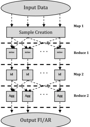
φ > δ. In the first stage, the samples are created and mined in par-allel and the so-obtained collections of Frequent Itemset are then aggregated in a second stage to compute the final output. This ap-proach is a perfect match for the MapReduce framework, given the limited number of synchronization and communication steps that are needed. Each stage is performed in a single MapReduce round. The computational and data workflow of PARMA is presented in Figure 1, which we describe in detail in the following paragraphs.
Computing
Nand
w.
From the above discussion it should be clear that, oncep,m,εandδhave been fixed, there is a trade-off betweenwandN. In the MapReduce setting, often the most ex-pensive operation is the movement of data between the mappers and the reducers in the shuffle phase. In PARMA, the amount of data to be shuffled corresponds to the sum of the sizes of the samples, i.e.,N w, and to the amount of communication needed in the aggre-gation stage. This second quantity is dependent on the number of frequent itemsets in the dataset, and therefore PARMA has nocon-
Sample Creation
mine mine mine Map 1 Reduce 1 Map 2 Agg Agg Agg Reduce 2. . .
. . .
Input Data
Output FI/AR
id id. . .
idFigure 1: A system overview of PARMA. In this diagram, el-lipses represent data, squares represent computations on that data and arrows show the movement of data through the sys-tem. The diagram is broken into 4 main computations which correspond to the Map and Reduce phases of the two MapRe-duce rounds in the algorithm. In the Map of Stage 1, a sample is created. In the Reduce of Stage 1, a mining algorithm is run on the subset of the sample created in the Map phase. This mining algorithm can be either frequent itemset mining or as-sociation rule mining, and as such is generically labeled mine. In the Map phase of Stage 2, the local frequent itemsets are sent to an identity mapper, and finally Aggregated in the Stage 2 Re-duce to get a global set of frequent itemsets or assocation rules, depending on the mining algorithm used.
trol over it. PARMA tries to minimize the first quantity when com-putingNandwin order to achieve the maximum speed. It is still possible to minimize for other quantities (e.g. εorδif they have not been fixed), but we believe the most effective and natural in the MapReduce setting is the minimization of the communication. This intuition was verified in our experimental evaluation, where com-munication proved to be the dominant cost. We can formulate the problem of minimizingN was the following Mixed Integer Non Linear Programming (MINLP) problem:
• Variables:non-negative integerN, realφ∈(0,1), • Objective:minimize2N/ε2(d+ log(1/φ)). • Constraints:
N≤p (2)
φ≥e−mε2/2+d (3)
N(1−φ)−p
N(1−φ)2 log(1/δ)≥N/2 + 1 (4)
Note that, because of our requirement2)onw, the sample sizew
is directly determined byφthrough Lemma 1, so the trade-off is really betweenNandφandwdoes not appear in the above prob-lem. Sinceφis a probability we restrict its domain to the interval
(0,1), but it must also be such that the single sample sizewis at mostm, as required by1)and expressed by Constraint (3). The limit to the number of samplesN is expressed by Constraint (2). The last constraint (4) is a bit more technical and the need for it will be evident in the analysis of the algorithm. Intuitively, it expresses the fact that an itemset must appear in a sufficiently high fraction of the collections obtained from the samples in the first stage in order to be included in the output collection. This fraction must be at least the half the number of samples. Due to the integrality constraint onN, this optimization problem is not convex, although when the constraint it is dropped the feasibility region is convex, and the objective function is convex. This means that is relatively easy and fast to find an integer optimal solution to the problem us-ing a global MINLP solver like BARON [31].
4.2
Description
In the following paragraphs we give a detailed description of PARMA. The reader is also referred to Figure 1 for a schematic rep-resentation of the data/computational overview of PARMA’s work-flow.
Stage 1: Sampling and Local Mining.
Onceφ,wandNhave been computed, PARMA enters the first MapReduce round to create theN samples (phase Map 1 in Figure 1) and mine them (Reduce 1). We see the input of the algorithm as a sequence
(1, τ1),(2, τ2),· · ·,(|D|, τ|D|),
where the τi are transactions inD. In the Map phase, the
in-put of themapfunction is a pair(tid, τ), wheretidis a natural from1to|D|andτ is a transaction inD. The map function pro-duces in output a pair(i,(`(τi), τ))for each sampleSicontaining
τ. The value`(τi) denotes the number of timesτ appears inSi,
1 ≤i≤N. We use random sampling with replacement and en-sure that all samples have sizew, i.e.,P
τ∈D` (i)
τ = w, ∀i. In
the Reduce phase, there are N reducers, with associated key i,
1 ≤ i ≤ N. The input to reducer iis(i,Si), 1 ≤ i ≤ N.
Reducerimines the setSiof transactions it receives using an
ex-act sequential mining algorithm like Apriori or FP-Growth and a lowered minimum frequency thresholdθ0 = θ −ε/2to obtain Ci=FI(Si,I, θ0). For each itemsetA∈ Cithe Reduce function
outputs a pair(A,(fSi(A),[fSi(A)−ε/2, fSi(A) +ε/2]).
Stage 2: Aggregation.
In the second round of MapReduce, PARMA aggregates the result from the first stage to obtain aε -approximation toFI(D,I, θ)with probability at least1−δ. The Map phase (Map 2 in Figure 1) is just the identity function, so for each pair(A,(fSi(A),[fSi(A)−ε/2, fSi(A) +ε/2])
in the input the same pair is produced in the output. In the Reduce phase (Reduce 2) there is a reducer for each itemsetAthat appears in at least one of the collectionsCj(i.e.,∀Asuch that there is aCj
containing a pair related toA). The reducer receives as input the itemsetAand the setFAof pairs
(fSi(A),[fSi(A)−ε/2, fSi(A) +ε/2])
for the samplesSisuch thatA∈ Ci. Now let
The itemsetA is declaredglobally frequentand will be present in the output if and only if|FA| ≥R. If this is the case, PARMA
computes, during the Reduce phase of the second MapReduce round, the estimationf˜(A)for the frequencyfD(A)of the itemsetAin
Dand the confidence intervalKA. The computation forf˜(A)
pro-ceeds as follows. Let[aA, bA]be theshortestinterval such that
there are at leastN −R+ 1elements from FA that belong to
this interval. The estimationf˜(A)for the frequencyfD(A)of the
itemsetAis the central point of this interval:
˜
f(A) =aA+
bA−aA
2
The confidence intervalKAis defined as
KA= h aA− ε 2, bA+ ε 2 i .
The output of the reducer assigned to the itemsetAis
(A,( ˜f(A),KA)).
The output of PARMA is the union of the outputs from all reducers.
4.3
Analysis
We have the following result:
LEMMA 3. The output of the PARMA is anε-approximation of
FI(D,I, θ)with probability at least1−δ.
PROOF. For each sampleSi, 1 ≤ i ≤ N we define a
ran-dom variableXithat takes the value1ifCi = FI(Si,I, θ0)is a
(ε, ε/2)-approximation ofFI(D,I, θ),Xi = 0otherwise. Given
our choices ofwand θ0, we can apply Lemma 1 and have that
Pr(Xi= 1)≥1−φ. LetY =PNr=1Xrand letZbe a random
variable distributed asB(N,1−φ). For any constantQ, we have
Pr(Y < Q)≤Pr(Z < Q). Also, for any constantQ < N(1−φ)
we have Pr(Y ≤Q)≤Pr(Z ≤Q)≤e−N(1−φ)(1− Q N(1−φ)) 2/2 ,
where the last inequality follows from an application of the Cher-noff bound [24, Chap. 4]. We then have, for our choice ofφandN
and forQ =R(defined in Eq. (5)), that with probability at least
1−δ, at leastRof the collectionsCiare(ε, ε/2)-approximations
ofFI(D,I, θ). Denote this event asG. For the rest of the proof we will assume thatGindeed occurs.
Then∀A ∈FI(D,I, θ),Abelongs to at leastRof the collec-tionsCi, therefore a triplet(A,f˜(A),KA)will be in the output of
the algorithm. This means that Property 1 from Def. 4 holds. Consider now any itemsetBsuch thatfD(B)< θ−ε. By
def-inition of(ε, ε/2)-approximation we have thatBcan only appear in the collectionsCithat are not(ε, ε/2)-approximations. Given
thatGoccurs, then there are at mostN−Rsuch collections. But from Constraint (4) and the definition ofRin (5), we have that
N−R < R, and thereforeBwill not be present in the output of PARMA, i.e. Property 2 from Def. 4 holds.
Let nowCbe any itemset in the output, and consider the interval
SC= [aC, bC]as computed by PARMA.SCcontains at leastN−
R+ 1of thefSi(C), otherwise C would not be in the output.
By our assumption on the eventG, we have that at leastRof the
fSi(C)’s are such that|fSi(C)−fD(C)| ≤ε/2. Then there is an
indexjsuch that|fSj(C)−fD(C)| ≤ε/2and such thatfSj(C)∈ SC. Given also thatfSj(C)≥aC, thenfD(C)≥aC−ε/2, and
analogously, given thatfSj(C) ≤bC, thenfD(C) ≤bC+ε/2.
This means that
fD(C)∈ h aC− ε 2, bC+ ε 2 i =KC, (6)
which, together with the fact thatf˜C∈ KCby construction, proves
Property 3.b from Def. 4. We now give a bound to|SC|=bC−
aC. From our assumption on the eventG, there are (at least)R
valuesfSi(C)such that|fSi(C)−fD(C)| ≤ε/2, then the interval [fD(C)−ε/2, fD(C) +ε/2]contains (at least)RvaluesfSi(C).
Its length ε is an upper bound to|SC|. Then the length of the
intervalKC= [aC−ε/2, bC+ε/2]is at most2ε, as requested by
Property 3.c from Def. 4. From this, from (6), and from the fact thatf˜(C)is the center of this interval we have|f˜(C)−fD(C)| ≤ ε, i.e., Property 3.a from Def. 4 holds.
4.4
Top-K Frequent Itemsets And Association
Rules
The above algorithm can be easily adapted to computing, with probability at least1−δ,ε-approximations toTOPK(D,I, K)and toAR(D,I, θ, γ). The main difference is in the formula to com-pute the sample sizew(Lemma 1), and in the process to extract the local collections from the samples. The case of top-Kis presented in [29] and is a minor modification of Lemma 1, while for the asso-ciation rule case we can use Lemma 2. These are minimal changes to the version of PARMA presented here, and the corresponding algorithms still achieve the same levels of guaranteed accuracy and confidence.
5.
IMPLEMENTATION
The entire PARMA algorithm has been coded as a Java library for Hadoop, the popular open source implementation of MapRe-duce. Because all experiments were done using Amazon Web Ser-vice (AWS) Elastic MapReduce, the version of Hadoop used was 0.20.205, the highest supported version by AWS. The choice to use Java was motivated on several grounds. First, the construction of a runnable jar file is the easiest way to run a distributed program with Hadoop. Second, a Java implementation allows future integration with the Apache Mahout parallel machine learning library [3], a widely used package among machine learning end-users and re-searchers alike. Apache Mahout also includes an implementation of PFP [18] that we have used for our evaluation of PARMA.
In PARMA, during the mining phase (i.e. during the reducer of stage 1), any frequent itemset or association rule mining algorithm can be used. We wanted to compare the performances of PARMA against PFP which only produces frequent itemsets, therefore we chose to use a frequent itemset mining algorithm instead of an as-sociation rule mining algorithm. Again, this choice was merely for ease of comparison with existing parallel frequent itemset mining algorithms as no such algorithms for association rule mining exist. While there are many frequent itemset mining algorithms available, we chose the FP-growth implementation provided by [7]. We chose FP-growth due to its relative performance superiority to other Fre-quent Itemsets mining algorithms. Additionally, since FP-growth is the algorithm that PFP has parallelized and uses internally, the choice of FP-growth for the mining phase in PARMA is appropri-ate for a more natural comparison.
We also compare PARMA against the naive distributed counting algorithm for computing frequent itemsets. In this approach, there is only a single MapReduce iteration. The map breaks a trans-actionτ into its powersetP(τ)and emits key/value pairs in the form(A,1)whereAis an itemset inP(t). The reducers simply count how many pairs the receive for each itemsetAand output the
number of items 1000 average transaction length 5 average size of maximal potentially large itemsets 5 number of maximal potentially large itemsets 5 correlation among maximal potentially large itemsets 0.1 corruption of maximal potentially large itemsets 0.1
Table 1: Parameters used to generate the datasets for the run-time comparison between DistCount and PARMA in Figure 2.
number of items 10000
average transaction length 10 average size of maximal potentially large itemsets 5 number of maximal potentially large itemsets 20 correlation among maximal potentially large itemsets 0.1 corruption of maximal potentially large itemsets 0.1
Table 2: Parameters used to generate the datasets for the run-time comparison between PFP and PARMA in Figure 3.
itemsets with frequency above the minimum frequency threshold. This is similar to the canonical wordcount example for MapRe-duce. However, because the size of the powerset is exponential in the size of the original transaction (specifically2|τ|, where|τ| denotes the number of items in a given transaction), this algorithm incurs massive network costs. This is very similar to the algorithms presented in [10, 19, 33]. We have built our own implementation of distributed counting in Java using the Hadoop API.
6.
EXPERIMENTS
The performance evaluation of PARMA was done using Ama-zon’s Elastic MapReduce platform. In particular, we used instance typem1.xlarge, which contains roughly 17GB of memory and 6.5 EC2 compute units. For data, we created artificial dataset using the synthetic data generator from [9]. This implementation is based on the generator described in [2]. Because this model for transactional data generation has been often used in frequent itemset and associ-ation rule mining papers, our results more widely comparable. The generator can be parameterized to generate a wide range of data. We used two distinct sets of parameters to generate the datasets. The first set was for the datasets in for the experiments between PARMA and the distributed counting algorithm (DistCount). These parameters are shown in Table 1. The next set of parameters was used in the generation of the large datasets for the runtime com-parison between PARMA and PFP. These parameters are shown in Table 2. The parameters were chosen to mimic real-world datasets on which PARMA would be run. For a full description of the rele-vant parameters, we refer the reader to [2]. Ideally, we would have tested DistCount using the same datasets as both PARMA and PFP. However, because the amount of data generated in the map phase of DistCount grows exponentially with the length of the individual transactions in the dataset, we found that DistCount would run out of memory using datasets with longer transactions. For this reason, we instead had to generate datasets with both shorter and less trans-actions for its comparisons. This is a strong testament to the lack of scalability of the distributed counting algorithm.
Because PARMA is an approximate algorithm, the choice of ac-curacy parametersεandδare important, as isθ, the minimum fre-quency at which itemsets were mined. In all of our experiments,
ε= 0.05andδ= 0.01. This means that the collection of itemsets mined by PARMA will be a 0.05-approximation with probability
0.99. In practice, we show later that the results are much more ac-curate than what this. For all experiments other than the minimum frequency performance comparison in Figure 6 and for the accu-racy comparison in Figures 8 and 9,θwas kept constant at 0.1.
We focus on three main aspects in the experimental analysis of PARMA. First is the runtime analysis. In this set of experiments we compare PARMA to PFP and DistCount using several differ-ent datasets of varying size and mined with varying minimum fre-quency thresholds. We then break down the runtime of PARMA into the map, reduce and shuffle phases of each of the two stages. This demonstrates which parts of the algorithm have runtimes that increase as the data size grows and which parts are relatively data independent. The second aspect is speedup, to show the scalability of our algorithm. Data size was held constant and PARMA was run using increasingly larger clusters of nodes. . Finally, because the output of PARMA is anε-approximation of the real set of frequent itemsets, we provide an accuracy analysis to verify that our results are indeed within the desired quality bounds.
6.1
Runtime Analysis
For the performance analysis of PARMA, we will analyze the relative performance against two exact frequent itemset mining al-gorithms on MapReduce,DistCountandPFP. We also provide a breakdown of the costs associated with each stage of PARMA.
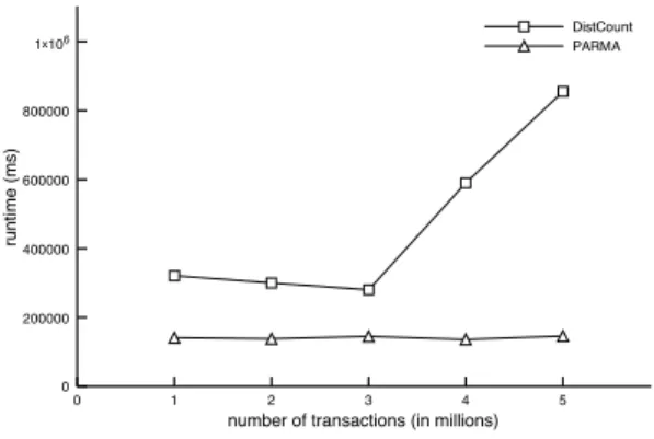
The results of the experiments between PARMA and DistCount are shown in Figure 2. As discussed previously, due to limitations in the scalability of DistCount, we were unable to test on the larger datasets, so the smaller datasets were used. Due to the nature of how DistCount mines itemsets, longer itemsets affect runtime the most, as the number of key/value pairs generated from each trans-action is exponential in the size of the transtrans-action. This is not to say that more transactions does not affect runtime, just that the length of those transactions also has a significant impact. Because of this, it is possible to have datasets with fewer transactions but with more “long” transactions to take longer to mine. This effect is seen in the first three datasets (1-3million). Even though the num-ber of transactions significantly increases, the relative length of the longest transactions was actually longer in the 1 million transac-tion dataset. Indeed, upon further inspectransac-tion, we found that the 1 million transaction dataset had 25 transactions over 20 items in length, while the 2 and 3 million transaction dataset had less than 15. Of course, since these datasets were generated independently and with the same parameters discussed above, this was purely by chance. However, as the dataset continues to increase, the exponen-tial growth in the number of intermediate key/value pairs is seen by the sharp increase in runtime. While we tried to test with a dataset with 6 million transaction, DistCount ran out of memory. The lack of ability to handle either long individual transactions or a large number of transactions in a dataset clearly limits DistCount’s real-world applicability. The runtime of PARMA is significantly faster than that of DistCount and, more importantly, nearly con-stant across dataset sizes. The reasons for this will be discussed in detail later.
For the performance comparison with PFP, 10 datasets were gen-erated using parameter values from Table 2 and ranging in size from 10 to 50 million transactions. All experiments were conducted us-ing a cluster of 8 m1.xlarge EC2 instances. The overall results can be seen in Figure 3. For every dataset tested, PARMA was able to mine the dataset roughly 30-55% faster than PFP. In real time, this performance gain is significant, as can be seen in Figure 3. The reason for the relative performance advantage of PARMA is twofold. The main reason is that for larger datasets the size of the dataset that PARMA has sampled (and mined) is staying the same,
0 1 2 3 4 5
number of transactions (in millions)
0 200000 400000 600000 800000 1x10⁶ ru n time (ms) DistCount PARMA
Figure 2: A comparison of runtimes of runtimes between Dist-Count and PARMA on an 8 node Elastic MapReduce cluster.
0 10 20 30 40 50
number of transactions (in millions)
0 100000 200000 300000 400000 runtime (ms) PFP PARMA
Figure 3: A runtime comparison between PFP and PARMA on an 8 node Elastic MapReduce cluser. Dataset size is varied from 5 to 50 million transactions, with each dataset being in-dependently generated using identical parameters. Runtime is measured as a sum of the runtime of all stages for each of the respective algorithms.
whereas PFP is mining more and more transactions as the dataset grows. The second reason is that as the dataset grows, PFP is po-tentially duplicating more and more transactions as it assigns trans-actions to groups. A transaction that belongs to multiple groups is sent to multiple reducers, resulting in higher network costs.
The most important aspect of the comparison of PFP to PARMA is that the runtimes as data grows are clearly diverging due to the reasons discussed above. While 50 million transactions is very siz-able, it is not hard to imagine real-world datasets with transactions on the order of billions. Indeed, many point-of-sale datasets would easily break this boundary. In these scenarios a randomized algo-rithm such as PARMA would show increasing performance advan-tages over exact algorithms such as any of the standard non-parallel algorithms or PFP, which must mine the entire dataset. At that scale, even transmitting that data over the network (several times in the case of PFP) would become prohibitive.
To understand the various costs of PARMA it is important to an-alyze the runtimes at each of the various stages in the algorithm. To do this, we have implemented runtime timers at very fine gran-ularities throughout our algorithm. The timers’ values are written to Hadoop job logs for analysis. This breakdown allows us to not only analyze the overall runtime, but also the sections of the algo-rithm whose runtimes are affected by an increase in data size. In
Figure 4, a breakdown of PARMA runtimes is shown for each of the six segments of the algorithm, which include a map, shuffle and reduce phase for each of the two stages. For readability concerns, we have chosen to show breakdown of only a subset of the datasets tested. It is important to note, that there was nothing to be gained from an analysis standpoint for showing the extra graphs. All pat-terns discussed continued for all datasets tested. The only outlier was the 5 million transaction dataset, and the reasons for this will be discussed later. This breakdown demonstrates several interest-ing aspects of PARMA. First, the cost of the mininterest-ing local frequent itemsets (stage 1, reduce) is relatively constant. For many frequent itemset mining implementations, this cost will grow with the size of the input. This is not the case in PARMA, because local frequent itemset mining is being done on constant-sized sample of the input. Indeed another interesting observation, as expected, is that the only cost that increases as sample size increases is the cost of sampling (stage 1, map). This is because in order to be sampled the input data must be read, so larger input data means larger read times. In practice, because this cost is minimal and grows linearly with the input, it will never be prohibitive in practice, especially considering all other current algorithms must read the entire input data at least once, and in many cases multiple times.
There is one outlier in the graph, which is the dataset with 5 mil-lion transactions. Because each dataset was independently gener-ated, it is possible for a dataset to have a larger number of frequent itemsets than other datasets, even if it has less transactions. This is the case with the 5 million transaction dataset. To see that this is indeed what is happening, we refer again to Figure 4. As expected, the sample generation phase (stage 1, map) is smaller relative to the larger datasets. However, the local frequent itemset mining phase (stage 1, reduce) is longer than any of the larger datasets. This is because there are more frequent itemsets in that dataset. This can also be seen in the relatively larger shuffle phase of stage 2, which is in charge of sending all equivalent local frequent itemsets to the same reducer for aggregation. Because there are more local item-sets present, this shuffle stage is larger than for the other dataitem-sets. Because the same dataset was used for the runtime of analysis of PFP and PARMA, and the overall runtimes of both should increase in a dataset with more frequent itemsets, we should see a higher runtime on the 5 million transaction dataset for PFP relative to its the other datasets, which is indeed the case. The runtime of PFP increases with both the size of the dataset as well as the number of frequent itemsets present, but it is not until a dataset of 25 million transactions that the runtime exceeds the runtime for the 5 million transaction dataset. This outlier is not a flaw with PARMA or PFP, but is a result of one of the inherent aspects of frequent itemset min-ing: it takes longer to mine datasets with more frequent itemsets.
In Figure 5, a breakdown of total runtimes is shown clustered by stage. In this view, it is apparent that most of the phases of the algorithm are nearly constant across data sizes. The obvious increase is the map of stage 1, which was discussed above. An-other slight runtime increase as data increases occurs in the shuffle phase of stage 2. Because there are more transactions in the larger datasets, there will be more frequent itemsets on average. In stage 2, an identity mapper sends each frequent itemset to the appropriate reducer for counting. Thus, all this data is being moved across the network, which is manifested in the shuffle phase of stage 2. The more frequent itemsets, the more data there is to shuffle across the network, which results in longer runtimes. Also, in Figure 5 we once again notice that the 5 million transaction dataset is an out-lier. The longer than expected phase is the shuffle phase of stage 2, which again suggests that this dataset took longer to mine because more frequent itemsets were found.
0 20000 40000 60000 80000 100000 120000 140000 160000 180000 5 10 15 20 run,me (ms) number of transac,ons (in millions) Stage 2 Reduce Stage 2 Shuffle Stage 2 Map Stage 1 Reduce Stage 1 Shuffle Stage 1 Map
Figure 4: Runtimes of the map/reduce/shuffle phases of PARMA. Run on an 8 node Elastic MapReduce cluster. For each dataset size, there are a total of 6 different runtimes: a map/reduce/shuffle phase for both stage 1 and stage 2. The sum of the runtimes of all phases is equivalent to the total runtime of the algorithm on that dataset.
0 10000 20000 30000 40000 50000 60000 70000 80000 90000 100000 Stage 1: 5 10 15 20 Stage 2: 5 10 15 20 run5me (ms) number of transac5ons (in millions) Reduce Shuffle Map
Figure 5: A Comparison of runtimes of the map/reduce/shuffle phases of PARMA, as a function of input dataset size. Clustered by stage. Run on an 8 node Elastic MapReduce cluster.
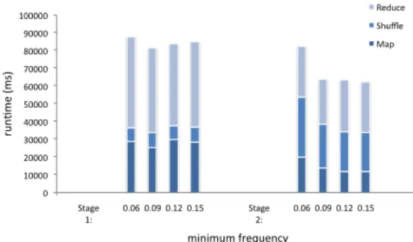
Figure 6 shows the a breakdown of PARMA runtimes as the min-imum frequency at which the data is mined at is changed. Data size was kept constant at 10 million transactions. Minimum frequency is used by the local frequent itemset mining algorithm to prune itemsets; itemsets below the minimum frequency are not consid-ered frequent, nor is any superset since a superset must, by defini-tion, contain the not frequent set and therefore cannot be frequent itself. Intuitively, a lower minimum frequency will mean more fre-quent itemsets are produced. Other than a runtime increase in the local frequent itemset mining phase (stage 1, reduce), the effects of this can be seen in the stage 2 shuffle phase as well, as there is more data to move across the network. Still, the added costs of mining with lower frequencies are relatively small.
6.2
Speedup
To show the speedup of PARMA, we used a two-nodes cluster as the baseline. Because PARMA is intended to be a parallel al-gorithm, the choice of a two-nodes cluster was more appropriate than the standard single node baseline. For the dataset, we used a 10 million transaction database generated using the parameters in Table 2. The results are shown in Figure 7. The three lines on this graph represent the relative speedup of both stage 1 and stage 2 as well as the overall PARMA algorithm. The graph indicates that stage 1 is highly parallelizable and follows a near-ideal speedup for up to 8 nodes, after which a slight degradation of speedup oc-curs. There are two reasons for this slight degradation. In the map phase of stage 1, due to an implementation decision in Hadoop, the
0 10000 20000 30000 40000 50000 60000 70000 80000 90000 100000 Stage 1: 0.06 0.09 0.12 0.15 Stage 2: 0.06 0.09 0.12 0.15 run6me (ms) minimum frequency Reduce Shuffle Map
Figure 6: A comparison of runtimes of the map/reduce/shuffle phases of PARMA, as a function of minimum frequency. Clus-tered by stage. Run on an 8 node Elastic MapReduce cluster.
2 4 6 8 10 12 14 16 number of instances 1 2 3 4 5 6 7 speedup ideal total Stage 1 Stage 2
Figure 7: The speedup analysis of PARMA. The analysis is bro-ken down into 2 stages. Stage 1 is local frequent itemset mining. Stage 2 is the aggregation of frequent itemsets into a global set of itemsets.
smallest unit of data that can be split is one HDFS block. As we continue to add more nodes to the cluster, we may have more avail-able map slots than HDFS data blocks, resulting in some slots being unused. Theoretically, this could be fixed by allowing smaller gran-ularity splitting in Hadoop. Another cause of the slightly sub-ideal speedup in stage 1 is from the reducer. Because the data in this experiment was held constant, the slight degradation in speedup as more than 8 nodes were added was a result of an inefficient over-splitting of transaction data. If each reducer in stage 1 is mining a very small subset of the transactions, the overhead of building the FP-tree begins to dominate the cost of mining the FP-tree. This is because the cost of mining the FP-tree is relatively fixed. Thus, we can “over-split” the data by forcing the reducer to build a large FP-tree only to mine a small set of transactions. For larger samples, the size of the cluster where speedup degradation begins to occur would also increase, meaning PARMA would continue to scale.
Also, as is clearly visible in the graph, the sub-ideal overall speedup is due largely to the poor speedup of stage 2. Stage 2 is bound almost entirely by the communication costs of transmitting the local frequent itemsets from stage 1 to the reducers that will do the aggregation. Because the amount of local frequent itemsets does not change as more nodes are added, the communication for this stage does not change. What does change is the number of itemsets each node must aggregate. During the reduce phase, each node is assigned a set of keys. All key/value pairs emitted from the map phase are sent to the reducer assigned their respective key.
The reducer is in charge of aggregating the values and emitting one aggregate value per key assigned to it. As more reducers are added to the cluster, each reducer will have fewer keys assigned to it, and therefore must aggregate across fewer values, resulting in faster ag-gregation. The very relative positive change in the line for stage 2 is a result of this slight speedup of the reduce phase.
A very important aspect of PARMA that should be stressed again here is that the size of the sample that will be mined does not de-pend directly on size of the original database, but instead on the confidence parametersεandδ. From a practical perspective, this means that assuming confidence parameters are unchanged, larger and larger datasets can be mined with very little increase in overall runtime (the added cost will only be the extra time spent reading the larger dataset initially during sampling). Because of this, clus-ters do not need to scale with the data, and often a relatively modest cluster size will be able to mine itemsets in a very reasonable time.
6.3
Accuracy
The output of PARMA is a collection of frequent itemsets which approximates the collection one can obtain by mining the entire dataset. Although our analysis shows that PARMA offers solid guarantees in terms of accuracy of the output, we conducted an ex-tensive evaluation to assess the actual performances of PARMA in practice, especially in relation to what can be analytically proved.
We compared the results obtained by PARMA with the exact col-lection of itemsets from the entire dataset, for different values of the parametersε,δ, andθ, and for different datasets. A first important result is that in all the runs, the collection computed by PARMA was indeed aε-approximation to the real one, i.e., all the properties from Definition 4 were satisfied. This fact suggests that the con-fidence in the result obtained by PARMA is actually greater than the level1−δsuggested by the analysis. This can be explained by considering that we had to use potentially loose theoretical bounds in the analysis to make it tractable.
Given that all real frequent itemsets were included in the out-put, we then focused on how many itemsets with real frequency in the interval[θ−ε, θ)were included in the output. It is important to notice that these itemsets would beacceptablefalse positives, as Definition 4 does not forbid them to be present in the output. We stress again that the output of PARMA never contained non-acceptablefalse positives, i.e. itemsets with real frequency less than the minimum frequency thresholdθ. The number of accept-able false positives included in the output of PARMA depends on the distribution of the real frequencies in the interval[θ−ε, θ), so it should not be judged in absolute terms. In Table 3 we report, for various values ofθ, the number of real frequent itemsets (i.e., with real frequency at leastθ, the number of acceptable false posi-tives (AFP) contained in the output of PARMA, and the number of itemsets with real frequency in the interval[θ−ε, θ), i.e., the max-imum number of acceptable false positives that may be contained in the output of PARMA (Max AFP). These numbers refers to a run of PARMA on (samples of) the 10M dataset, withε = 0.05
andδ = 0.01. It is evident that PARMA does a very good job in filtering out even acceptable false positives, especially at lower fre-quencies, when their number increases. This is thanks to the fact that an itemset is included in the output of PARMA if and only if it appears in the majority of the collections obtained in the first stage. Itemsets with real frequencies in[θ−ε, θ)are not very likely to be contained in many of these collections.
We conducted an evaluation of the accuracy of two other com-ponents of the output of PARMA, namely the estimated frequen-cies for the itemsets in the output and the width of the confidence bounds for these estimations. In Figure 8 we show the distribution
θ Real FI’s Output AFP’s Max AFP’s
0.06 11016 11797 201636
0.09 2116 4216 10723
0.12 1367 335 1452
0.15 1053 299 415
Table 3: Acceptable False Positives in the output of PARMA
0.00E+00 5.00E-‐04 1.00E-‐03 1.50E-‐03 2.00E-‐03 2.50E-‐03 3.00E-‐03 0.06 0.09 0.12 0.15 ab solut e f re que nc y e rr or
minimum frequency threshold
Figure 8: Error in frequency estimations as frequency varies.
of the absolute error in the estimation, i.e.|f˜(X)−fD(X)|for all
itemsetsX in the output of PARMA, asθvaries. The lower end of the “whisker” indicates the minimum error, the lower bound of the box corresponds to the first quartile, the segment across the box to the median, and the upper bound of the box to the third quar-tile. The top end of the whisker indicates the maximum error, and the central diamond shows the mean. This figure (and also Fig-ure 9) shows the values for a run of PARMA on samples of the 10M dataset, withε= 0.05andδ = 0.01. We can see that even the maximum values are one order of magnitued smaller than the threshold of0.05guaranteed by the analysis, and many of the er-rors are two or more orders of magnitude smaller. It is also possible to appreciate that the distribution of the error would be heavily con-centrated in a small interval if the maximum error were not so high, effectively an outlier. The fact that the average and the median of the error, together with the entire “box” move down as the mini-mum frequency threshold decrease can be explained by the fact that at lower frequencies more itemsets are considered, and this makes the distribution less susceptible to outliers. This is a sign not only of the high level of accuracy achieved by PARMA, but also of the consistency in achieving such a level across a very large portion of the output.
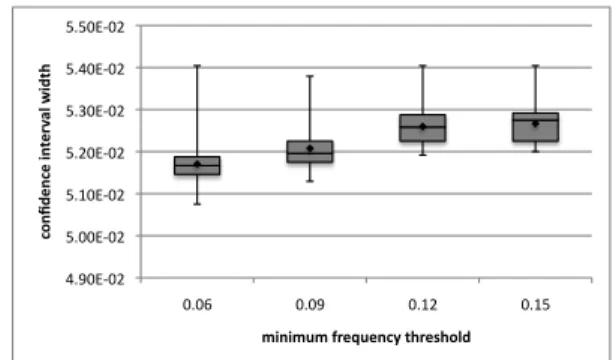
Finally, in Figure 9 we show the distribution of the widths of the confidence intervalsK(A)for the frequency estimationsf˜(A)of
4.90E-‐02 5.00E-‐02 5.10E-‐02 5.20E-‐02 5.30E-‐02 5.40E-‐02 5.50E-‐02 0.06 0.09 0.12 0.15 co nfi de nc e in te rv al w id th
minimum frequency threshold
the itemsetsAin the output of PARMA. Given thatε= 0.05, the maximum allowed width was2ε= 0.1. It is evident from the fig-ures that PARMA returns much narrower intervals, of size almost
ε. Moreover, the distribution of the width is very concentrated, as shown by the small height of the boxes, suggesting that PARMA is extremely consistent in giving very high quality confidence inter-vals for the estimations. We state again that in all runs of PARMA in our tests, all the confidence intervals contained the estimation and the real frequency, as requested by Definition 4. As seen in the case of the estimation error, the distribution of the widths shifts down at lower thresholdsθ. This is motivated by the higher num-ber of itemsets in the output of PARMA at those frequencies. Their presence makes the distribution more robust to outliers. Thanks to this fact we can conclude that PARMA gives very narrow but extremely accurate confidence intervals across the entirety of its output.
This analysis of the accuracy of various aspects of PARMA’s output shows that PARMA can be very useful in practice, and the confidence of the end user in the collections of itemsets and estima-tions given in its output can be even higher than what is guaranteed by the analysis.
7.
CONCLUSIONS
In this paper, we have described PARMA, a parallel algorithm for mining quasi-optimal collections of frequent itemsets and asso-ciation rules in MapReduce. We showed through theoretical anal-ysis that PARMA offers provable guarantees on the quality of the output collections. Through experimentation on a wide range of datasets ranging in size from 5 million to 50 million transactions, we have demonstrated a 30-55% runtime improvement over PFP, the current state-of-the-art in exact parallel mining algorithms on MapReduce. Empirically we were able to verify the accuracy of the theoretical bounds, as well as show that in practice our results are orders of magnitude more accurate than is analytically guaran-teed. Thus PARMA is an algorithm that can scale to arbitrary data sizes while simultaneously providing nearly perfect results.
8.
REFERENCES
[1] R. Agrawal, T. Imieli´nski, and A. Swami. Mining association rules between sets of items in large databases.SIGMOD Rec., 22:207–216, June 1993.
[2] R. Agrawal and R. Srikant. Fast algorithms for mining association rules in large databases. InProceedings of the 20th International Conference on Very Large Data Bases, VLDB ’94, pages 487–499, San Francisco, CA, USA, 1994. Morgan Kaufmann Publishers Inc.
[3] Apache Mahout.http://mahout.apache.org/. [4] G. Buehrer, S. Parthasarathy, S. Tatikonda, T. Kurc, and
J. Saltz. Toward terabyte pattern mining: an
architecture-conscious solution. InProceedings of the 12th ACM SIGPLAN symposium on Principles and practice of parallel programming, PPoPP ’07, pages 2–12, New York, NY, USA, 2007. ACM.
[5] F. Chierichetti, R. Kumar, and A. Tomkins. Max-cover in Map-Reduce. InProceedings of the 19th international conference on World wide web, WWW ’10, pages 231–240, New York, NY, USA, 2010. ACM.
[6] C.-T. Chu, S. K. Kim, Y.-A. Lin, Y. Yu, G. R. Bradski, A. Y. Ng, and K. Olukotun. Map-Reduce for machine learning on multicore. In B. Sch¨olkopf, J. C. Platt, and T. Hoffman, editors,Advances in Neural Information Processing Systems 19, Proceedings of the Twentieth Annual Conference on
Neural Information Processing Systems, Vancouver, British Columbia, Canada, December 4-7, 2006, pages 281–288. MIT Press, 2007.
[7] F. Coenen. The LUCS-KDD FP-growth association rule mining algorithm.
[8] S. Cong, J. Han, J. Hoeflinger, and D. Padua. A sampling-based framework for parallel data mining. In Proceedings of the tenth ACM SIGPLAN symposium on Principles and practice of parallel programming, PPoPP ’05, pages 255–265, New York, NY, USA, 2005. ACM.
[9] L. Cristofor. ARTool.
http://www.cs.umb.edu/˜laur/ARtool/, 2006.
[10] J.-D. Cryans, S. Ratt´e, and R. Champagne. Adaptation of APriori to MapReduce to build a warehouse of relations between named entities across the web. InAdvances in Databases Knowledge and Data Applications (DBKDA), 2010 Second International Conference on, pages 185–189, april 2010.
[11] J. Dean and S. Ghemawat. MapReduce: Simplified data processing on large clusters.Communications of the ACM, 51(1):107–113, 2008.
[12] M. El-Hajj and O. Zaiane. Parallel leap: large-scale maximal pattern mining in a distributed environment. InParallel and Distributed Systems, 2006. ICPADS 2006. 12th International Conference on, volume 1, page 8 pp., 0-0 2006.
[13] W. Fang, K. K. Lau, M. Lu, X. Xiao, C. K. Lam, Y. Yang, B. He, Q. Luo, P. V. Sander, and K. Yang. Parallel data mining on graphics processors. Technical Report 07, The Hong Kong University of Science & Technology, 2008. [14] A. Ghoting, P. Kambadur, E. Pednault, and R. Kannan.
NIMBLE: a toolkit for the implementation of parallel data mining and machine learning algorithms on mapreduce. In Proceedings of the 17th ACM SIGKDD international conference on Knowledge discovery and data mining, KDD ’11, pages 334–342, New York, NY, USA, 2011. ACM. [15] M. T. Goodrich, N. Sitchinava, and Q. Zhang. Sorting,
searching, and simulation in the MapReduce framework. CoRR, abs/1101.1902, 2011.
[16] S. Hammoud.MapReduce Network Enabled Algorithms for Classification Based on Association Rules. PhD thesis, Brunel University, 2011.
[17] J. Han, J. Pei, and Y. Yin. Mining frequent patterns without candidate generation.SIGMOD Rec., 29:1–12, May 2000. [18] H. Li, Y. Wang, D. Zhang, M. Zhang, and E. Y. Chang. PFP:
Parallel FP-Growth for query recommendation. In
Proceedings of the 2008 ACM conference on Recommender systems, RecSys ’08, pages 107–114, New York, NY, USA, 2008. ACM.
[19] L. Li and M. Zhang. The strategy of mining association rule based on cloud computing. InBusiness Computing and Global Informatization (BCGIN), 2011 International Conference on, pages 475–478, july 2011.
[20] Y. Li and R. Gopalan. Effective sampling for mining association rules. In G. Webb and X. Yu, editors,AI 2004: Advances in Artificial Intelligence, volume 3339 ofLecture Notes in Computer Science, pages 73–75. Springer, Berlin / Heidelberg, 2005.
[21] J. Lin and M. Schatz. Design patterns for efficient graph algorithms in mapreduce. InProceedings of the Eighth Workshop on Mining and Learning with Graphs, MLG ’10, pages 78–85, New York, NY, USA, 2010. ACM.
[22] L. Liu, E. Li, Y. Zhang, and Z. Tang. Optimization of frequent itemset mining on multiple-core processor. In Proceedings of the 33rd international conference on Very large data bases, VLDB ’07, pages 1275–1285. VLDB Endowment, 2007.
[23] H. Mannila, H. Toivonen, and I. Verkamo. Efficient algorithms for discovering association rules. InKDD Workshop, pages 181–192, Menlo Park, CA, USA, 1994. The AAAI Press.
[24] M. Mitzenmacher and E. Upfal.Probability and computing -randomized algorithms and probabilistic analysis.
Cambridge University Press, 2005.
[25] E. Ozkural, B. Ucar, and C. Aykanat. Parallel frequent item set mining with selective item replication.Parallel and Distributed Systems, IEEE Transactions on,
22(10):1632–1640, oct. 2011.
[26] S. Parthasarathy. Efficient progressive sampling for association rules. InProceedings of the 2002 IEEE
International Conference on Data Mining, ICDM ’02, pages 354–361. IEEE Computer Society, 2002.
[27] A. Pietracaprina, G. Pucci, M. Riondato, F. Silvestri, and E. Upfal. Space-round tradeoffs for MapReduce computations.CoRR, abs/1111.2228, 2011.
[28] A. Pietracaprina, M. Riondato, E. Upfal, and F. Vandin. Mining top-K frequent itemsets through progressive sampling.Data Mining and Knowledge Discovery, 21:310–326, 2010.
[29] M. Riondato and E. Upfal. Efficient discovery of association rules and frequent itemsets through sampling with tight performance guarantees.CoRR, abs/1111.6937, November
2011.
[30] J. Ruoming, Y. Ge, and G. Agrawal. Shared memory parallelization of data mining algorithms: techniques, programming interface, and performance.Knowledge and Data Engineering, IEEE Transactions on, 17(1):71 – 89, jan. 2005.
[31] N. V. Sahinidis and M. Tawarmalani.BARON 9.0.4: Global Optimization of Mixed-Integer Nonlinear Programs,User’s Manual, 2010.
[32] H. Toivonen. Sampling large databases for association rules. InProceedings of the 22th International Conference on Very Large Data Bases, VLDB ’96, pages 134–145, San Francisco, CA, USA, 1996. Morgan Kaufmann Publishers Inc.
[33] X. Y. Yang, Z. Liu, and Y. Fu. MapReduce as a programming model for association rules algorithm on Hadoop. In Information Sciences and Interaction Sciences (ICIS), 2010 3rd International Conference on, pages 99–102, june 2010. [34] M. Zaki. Parallel and distributed association mining: a
survey.Concurrency, IEEE, 7(4):14 –25, oct-dec 1999. [35] M. Zaki, S. Parthasarathy, W. Li, and M. Ogihara. Evaluation
of sampling for data mining of association rules. In Proceedings of the Seventh International Workshop on Research Issues in Data Engineering, RIDE ’97, pages 42 –50. IEEE Computer Society, apr 1997.
[36] L. Zhou, Z. Zhong, J. Chang, J. Li, J. Huang, and S. Feng. Balanced parallel FP-Growth with MapReduce. In
Information Computing and Telecommunications (YC-ICT), 2010 IEEE Youth Conference on, pages 243–246, nov. 2010.