Simulated Classical Tests in the Multiperiod Multinomial Probit Model

econstor

www.econstor.eu

Nutzungsbedingungen:

Die ZBW räumt Ihnen als Nutzerin/Nutzer das unentgeltliche, räumlich unbeschränkte und zeitlich auf die Dauer des Schutzrechts beschränkte einfache Recht ein, das ausgewählte Werk im Rahmen der unter

→ http://www.econstor.eu/dspace/Nutzungsbedingungen nachzulesenden vollständigen Nutzungsbedingungen zu vervielfältigen, mit denen die Nutzerin/der Nutzer sich durch die erste Nutzung einverstanden erklärt.

Terms of use:

The ZBW grants you, the user, the non-exclusive right to use the selected work free of charge, territorially unrestricted and within the time limit of the term of the property rights according to the terms specified at

→ http://www.econstor.eu/dspace/Nutzungsbedingungen By the first use of the selected work the user agrees and declares to comply with these terms of use.

Ziegler, Andreas

Working Paper

Simulated Classical Tests in the

Multiperiod Multinomial Probit Model

ZEW Discussion Papers, No. 02-38 Provided in cooperation with:

Zentrum für Europäische Wirtschaftsforschung (ZEW)

Suggested citation: Ziegler, Andreas (2002) : Simulated Classical Tests in the Multiperiod Multinomial Probit Model, ZEW Discussion Papers, No. 02-38, http:// hdl.handle.net/10419/24769

ZEW

Zentrum für Europäische Wirtschaftsforschung GmbH C e n t r e f o r E u r o p e a n E c o n o m i c R e s e a r c h

Discussion Paper No. 02-38

Simulated Classical Tests in the

Multiperiod Multinomial Probit Model

Discussion Paper No. 02-38

Simulated Classical Tests in the

Multiperiod Multinomial Probit Model

Andreas Ziegler

Die Discussion Papers dienen einer möglichst schnellen Verbreitung von neueren Forschungsarbeiten des ZEW. Die Beiträge liegen in alleiniger Verantwortung

der Autoren und stellen nicht notwendigerweise die Meinung des ZEW dar. Discussion Papers are intended to make results of ZEW research promptly available to other economists in order to encourage discussion and suggestions for revisions. The authors are solely

responsible for the contents which do not necessarily represent the opinion of the ZEW. Download this ZEW Discussion Paper from our ftp server:

Non-technical summary

In empirical economics, it is often necessary to use discrete choice models with more than two alternatives of a qualitative variable. Examples are the examination of the choice of modes for the journey to work, the household portfolio choice, the choice of living arrange-ments, or the brand choice of consumers. In these discrete choice models, intertemporal relationships should be included if panel data are available. Multiperiod multinomial pro-bit models are generally suitable for the analysis of such economic problems because of the flexible structure in these approaches. For a long time, the application of the multiperiod multinomial probit model was restricted because of the occurring multiple integrals. But by combining classical estimation methods and simulators, the use of such approaches has become feasible. When the multiperiod multinomial probit model is estimated in practice, the application of the simulated maximum likelihood method, e.g. the simulated counter-part of the maximum likelihood method, including the so-called GHK simulator, seems to be preferable. Asymptotic properties of the simulated maximum likelihood estimator as well as properties with finite numbers of observations and with finite numbers of random draws in the GHK simulator have been considered in the past.

The focus of this paper, however, is not on parameter estimation but on classical testing in the multiperiod multinomial probit model. By examining groups of variance-covariance parameters of the stochastic model components, special probit models can be tested. Note that the use of the Wald test, the score test, and the likelihood ratio test in complex multi-period multinomial probit models is computationally not feasible because of the appearing multiple integrals. But according to the inclusion of simulators into the maximum likeli-hood method, classical tests can also be associated with simulators. Thus, on the basis of simulated maximum likelihood estimates, one can construct simulated classical tests. The asymptotic properties of the simulated counterparts of the classical test statistics have been discussed in detail in the work of Lee (1999). But in view of the empirical application of simulated classical tests, the properties with finite numbers of observations and with finite numbers of random draws in the GHK simulator are more important than the asymptotic properties.

Hence, within the framework of Monte Carlo experiments, the present paper systematically compares different versions of the simulated Wald test, the simulated score test, and the simulated likelihood ratio test in the multiperiod multinomial probit model. Exemplarily, the five-period three-alternative probit model is considered here. The comparative analysis refer to the deviations of the frequency of type I errors from the basic significance levels as well as to the frequency of type II errors. In view of the empirical practice, the number of observations and the number of random draws in the GHK simulator are varied. One important finding is

that in contrast to the investigations of Lee (1999) in multiperiod binary probit models, the inclusion of the quasi maximum likelihood theory into the simulated classical tests and in particular into the simulated likelihood ratio test is not advantageous in general. Instead, the simple form of the simulated likelihood ratio test provides the comparatively most favorable results. Furthermore, neither the number of observations nor the number of random draws in the GHK simulator have a systematic effect on the frequency of type I errors. An increase in the number of observations only reduces the frequency of type II errors.

Simulated Classical Tests in the Multiperiod

Multinomial Probit Model

Andreas Ziegler

Centre for European Economic Research (ZEW)

Department of Environmental and Resource Economics,

Environmental Management

P.O. Box 103443, 68034 Mannheim, Germany

E-Mail: [email protected]

June 10, 2002

Abstract

This paper compares different versions of the simulated counterparts of the Wald test, the score test, and the likelihood ratio test in the multiperiod multinomial probit model. Monte Carlo experiments show that the simple form of the simulated likelihood ratio test delivers the most favorable test results in the five-period three-alternative probit model considered here. This result applies to the deviation of the frequency of type I errors from the given significance levels as well as to the frequency of type II errors. In contrast, the inclusion of the quasi maximum likelihood theory into the simulated likelihood ratio test leads to substantial computational problems. The combination of this theory with the simulated Wald test or the simulated score test also produces no general advantages over the other versions of these two simulated classical tests. Neither an increase in the number of observations nor a rise in the number of random draws in the considered GHK simulator systematically lead to a more precise con-formity between the frequency of type I errors and the basic significance levels. An increase in the number of observations merely reduces the frequency of type II errors.

Keywords: Simulated classical tests, multiperiod multinomial probit model, Monte Carlo simulation

JEL Codes: C12, C15, C25

∗_{I would like to thank Axel B¨orsch-Supan, Elke Eberts, Angelika Eymann, Fran¸cois Laisney, Klaus}

1

Introduction

By combining classical estimation methods and simulators, the application of flexible mul-tiperiod binary or one- or mulmul-tiperiod multinomial probit models has been feasible for quite a while in spite of the appearance of multiple integrals (see e.g. Lerman and Manski, 1981, McFadden, 1989, B¨orsch-Supan and Hajivassiliou, 1993, Keane, 1994, Hajivassiliou and McFadden, 1998). Examples for the empirical use of simulated classical estimations are Chintagunta, 1992, B¨orsch-Supan et al., 1992, Hajivassiliou, 1994, Bolduc et al., 1996, or Asea and Turnovsky, 1998. When such complex (particularly multinomial) probit models are estimated in practice, the simulated maximum likelihood method (SMLM), that is the simu-lated counterpart of the maximum likelihood method (MLM), including the GHK simulator, seems to be the most advantageous approach among the multitude of approaches suggested in the literature. This can be explained by the favorable computational properties of the SMLM and the high precision of the GHK simulator, but in particular by the fact that this simulated estimation method has also been implemented in some software packages, such as GAUSSX and LIMDEP.

Moreover, in different probit models, the properties of the SMLM estimator have been in-vestigated with finite numbers of observations and with finite numbers of random draws in the GHK simulator within the framework of Monte Carlo experiments (see e.g. Keane, 1994, Lee, 1997a, Inkmann, 2000, in multiperiod binary probit models, B¨orsch-Supan and Haji-vassiliou, 1993, Geweke et al., 1994, Stern, 2000, in one-period multinomial probit models, Geweke et al., 1997, in multiperiod multinomial probit models, Ziegler and Eymann, 2001, in one- and multiperiod multinomial probit models). Compared to the known asymptotic properties of the SMLM estimator, these systematic analyses are essential for the practical evaluation of estimation results in the empirical work.

The focus of this paper, however, is not on parameter estimation, but on classical testing in probit models. The basis for a traditional classical test is the corresponding MLM estimate. In flexible multiperiod binary or one- or multiperiod multinomial probit models, however, the MLM estimation is computationally not feasible because of the occurrence of multiple integrals. For this reason, also the application of the three classical tests is not possible in such complex probit models. The Wald test, the score test, and the likelihood ratio test can merely be practiced in special simple probit models in which an MLM estimation is feasible. But simulators can also be combined with classical tests pertinent to the inclusion of simulators into the MLM. Thus, on the basis of SMLM estimates, it is possible to construct simulated classical tests.

These kinds of tests refer to either a single parameter or to several parameters together. In the first case, by using the simulated counterpart of the z-test, it can be tested if a

choice depends on a single explanatory variable or if it depends on single contemporary or intertemporal relationships within the framework of flexible probit models. By examining groups of variance-covariance parameters of the stochastic model components, special probit models can be tested. In previous empirical SMLM estimations in probit models, particularly simulated z-tests have been regularly used, but special probit models have also been tested with the simulated counterparts of classical tests (see e.g. B¨orsch-Supan et al., 1992, Bolduc et al., 1996, and Inkmann, 2000). However, the problem of including simulators in these tests has been completely neglected. Only the asymptotic properties of different versions of simulated classical test statistics have been discussed in detail in the seminal work of Lee (1999).

In contrast, systematic Monte Carlo experiments that are extremely important for practical use in the empirical work, have seldom been performed with simulated classical tests in probit models. Even an analysis of (unsimulated) classical tests on the basis of MLM estimates in simple probit models is rare (so e.g. Davidson and MacKinnon, 1984, Guilkey and Murphy, 1993, Lechner, 1995, in one- or multiperiod binary probit models). To my knowledge, the only Monte Carlo experiments with simulated classical tests of several parameters together in probit models (resp. in more flexible discrete choice models) can be found in Lee (1997b, 1999), whereas Ziegler (2001) merely examines the special case of simulated z-tests. Lee (1999) exclusively investigates multiperiod binary probit models, however. Thus, he does not consider multinomial probit models. But these models are very important in empirical economics, for example in researching the choice of living arrangements or the consumer brand choice, in particular in multiperiod approaches (if panel data are available).

Therefore, in this study, various versions of simulated classical tests in the multiperiod multi-nomial probit model (MMPM) based on constrained and/or unconstrained SMLM estimates are examined. Due to its favorable properties, only the GHK simulator is included both in the basic SMLM estimation and in the final derivation of the test statistics. Within the framework of a flexible MMPM, two special MMPM are tested. By using several versions of the simulated estimation of the information matrix (i.e. the exclusive inclusion of the Hessian matrix of the simulated loglikelihood function, the exclusive inclusion of the gradi-ents of the simulated loglikelihood function, or the inclusion of both the gradigradi-ents and the Hessian matrix as pertinent to the quasi maximum likelihood theory according to White, 1982), one obtains different versions of the simulated Wald test and the simulated score test. In addition, the ideas of the quasi maximum likelihood theory can also be included in the simulated likelihood ratio test.

Exemplarily, according to the empirical application of B¨orsch-Supan et al. (1992), the five-period three-alternative probit model is considered in this study. In this framework, the (null) hypothesis that no contemporary relationships are present and the (null) hypothesis that no

autoregressive correlations are present in the stochastic model components are tested. The comparative analysis of the various versions of simulated classical tests refers to the deviation of the frequency of type I errors from the basic significance levels as well as to the frequency of type II errors. In view of the empirical work, the number of observations in addition to the number of random draws in the GHK simulator is varied here. In contrast, Lee (1999) only analyzes one number of observations.

In the investigations of Lee (1999), the inclusion of the quasi maximum likelihood theory into the simulated classical tests is advantageous. Moreover, a better conformity between the frequency of type I errors and the given significance levels results from a rise in the number of random draws in the GHK simulator. These outcomes cannot be confirmed by the Monte Carlo experiments in the present study. The number of random draws in the GHK simulator has no systematic influence both on the frequency of type I errors and on the frequency of type II errors. In addition, an increase in the number of observations merely reduces the frequency of type II errors. Most notably is, however, that there arise no general advantages from including the quasi maximum likelihood theory. Instead, by combining this theory and the simulated likelihood ratio test, substantial problems emerge in the calculation of the corresponding test statistic. In contrast to the analysis of Lee (1999), the simple form of the simulated likelihood ratio test delivers the comparatively most favorable results in the five-period three-alternative probit model considered here.

The structure of this paper is as follows: In the second section, the SMLM estimation in flexible MMPM is illustrated. On this basis, different versions of the simulated classical test statistics in MMPM are explained in the third section. In the fourth section, the design of the Monte Carlo experiments is described. The results of these analyses are discussed in the fifth section. The final section summarizes the results and draws some conclusions.

2

Simulated maximum likelihoood estimation in

mul-tiperiod multinomial probit models

Assume that an agent i (i = 1, . . . , N) chooses in each of the considered time periods

t = 1, . . . , T among a finite number J of mutually exclusive alternatives of a qualitative

variable. Ifichooses intthe alternativej, then the following hypothetical utility is obtained:

υijt =β

0

xijt+εijt i= 1, . . . , N;j = 1, . . . , J;t= 1, . . . , T (1)

The utility υijt depends on the vector of explanatory variables xijt = (xijt1, . . . , xijtK)0 and

on the corresponding parameter vector β = (β1, . . . , βK)0. In the following, the xijt are

vector Xi = (x0i1, . . . , x0iT)0. One obtains the MMPM if the stochastic utility components εijt are jointly normally distributed: εi = (εi11, . . . , εiJ1, . . . , εi1T, . . . , εiJT)

0

∼ NV(0; Σ). The random vectors εi are independent of each other and are independent of allXi. Diverse

versions of the MMPM result from various restrictions on the variance-covariance matrix Σ. In this paper, the stochastic utility components εijt allow any contemporary relationship

between the alternatives j as well as time invariant stochastic effects and intertemporal autoregressive correlations (see also Ziegler and Eymann, 2001), that is

εijt=αij +ζijt i= 1, . . . , N;j = 1, . . . , J;t = 1, . . . , T (2)

with

ζijt =ρjζi,j,t−1+

q

1−ρj2ηijt

whereby ηijt ∼ NV(0;σ2ηj) holds for t = 0,1, . . . , T, and the ηijt are uncorrelated over all

periods. For t = 1, . . . , T it is (∀j, j0_{) cov(η}

ijt, ηij0_t) = σ_η

jj0. The ρj denote the autocorre-lation coefficients for category j (where |ρj| < 1). Moreover, αij ∼ NV(0;σα2j) holds with

cov(αij, αij0) = σ_α

jj0, whereby theαij andζijtare uncorrelated with each other. Finally, it

fol-lows for the components of the variance-covariance matrix Σ of εi (withi= 1, . . . , N;j, j0 =

1, . . . , J;t, t0 _{= 1, . . . , T and t≥t}0_): cov(εijt, εij0_t0) = σ_α jj0 +ρj (t−t0₎ q 1−ρj2 q 1−ρj02 1−ρjρj0 σηjj0 (3)

In the present study, the coefficientsσ2

ηJ andσ

2

ηJ−1 are constrained to the value one, and the

coefficients σηjJ (∀j 6= J) are constrained to the value zero in order to be able to formally

identify the model. The parameters σ2

αJ and σαjj0 (∀j 6= j0) of the stochastic effects and the autocorrelation coefficient ρJ are also constrained to the value zero. Note that due to

practical aspects in the basic SMLM estimations of this study, the corresponding standard deviations σηj (j = 1, . . . , J −2) and σαj (j = 1, . . . , J −1) and the correlation coefficients

corr(ηijt, ηij0_t) = σ_η

jj0/σηjσηj0 (j, j

0 _{= 1, . . . , J −1;j 6= j}0_{) are used instead of the variances}

σ2

ηj and σ

2

αj and the covariances σηjj0. For this reason, the tested hypotheses refer to these

transformed parameters in this study.

In the following, all free coefficients of the considered MMPM are summarized in the vector

θ = (θ1, θ2, . . .)0. Over time, every observation i must choose between JT different category

sequences. For this reason, with regard to a chosen category sequence s, i chooses in every period the alternative that offers the highest utility according to the stochastic maximization hypothesis. In the flexible MMPM, the resulting probability Pis(θ) that an agent i chooses

the category sequence s is characterized by a (J −1)·T-dimensional integral.

Such choice probabilitiesPis(θ) can be quickly and accurately approximated with (unbiased)

numbers (see e.g. the overviews in Hajivassiliou et al., 1996, Vijverberg, 1997). By including such a simulator, one obtains the simulated counterpart Peis(θ) of Pis(θ). In comparative

Monte Carlo experiments, the so-called GHK (Geweke-Hajivassiliou-Keane) simulator (see B¨orsch-Supan and Hajivassiliou, 1993, Geweke et al., 1994, Keane, 1994) has proven to be superior to other simulators with regard to the approximation to the true probability (see also M¨uhleisen, 1994). For this reason, only this simulation method is considered in this study.

By linking an (unbiased) simulator to the MLM, one obtains the SMLM (see e.g. Gouri´eroux and Monfort, 1993). In the following, theJT_{-dimensional vectorY}

i = (Yi1, Yi2, . . .)0 contains

the observable endogenous variables

Yis =

  

1 if observation i chooses category sequence s

0 else

where s∈S and S represents the set of all JT _{potential category sequences. By embedding}

the simulatorPeis(θ) into the MLM approach and by consideringN independent pairs (Yi, Xi)

in the MMPM, one obtains the particular SMLM estimator: ˆ θ= (ˆθ1,θˆ2, . . .)0 = arg max θ "_N X i=1 X s∈S YislnPeis(θ) # (4) In the following, the parameter vector of the DGP is labelled ˙θ =³θ˙1,θ˙2, . . .

´₀

.

Note that the parameters in the iterative maximization process can take values that are outside of the domain. Due to this problem, the specially developed GAUSS programs take advantage of the fact that the MLM is invariant to reparameterizations of a model. Thus, for the free variance-covariance parameters of the MMPM, the following parameterizations are made at the beginning of the SMLM estimation:

lnση1, . . . ,lnσηJ−2 ln " 1 +corr(ηijt, ηij0_t) 1−corr(ηijt, ηij0_t) # (∀j 6=j0;j, j0 6=J) lnσα1, . . . ,lnσαJ−1 ln à 1 +ρ1 1−ρ1 ! , . . . ,ln à 1 +ρJ−1 1−ρJ−1 !

Subsequently, these transformed coefficients are entered into the optimization process. In the iterative adjustment of the variance-covariance matrix Σ of εi, as well as in the derivation of

the SMLM estimates after the maximization process, the corresponding reparameterizations are undertaken:

exphlnση1 i , . . . ,exphlnσηJ−2 i exp ½ ln · 1+corr(ηijt,ηij0t) 1−corr(ηijt,ηij0t) ¸¾ −1 exp ½ ln · 1+corr(ηijt,ηij0t) 1−corr(ηijt,ηij0t) ¸¾ + 1 (∀j 6=j0;j, j0 6=J) exphlnσα1 i , . . . ,exphlnσαJ−1 i exphln³1+ρ1 1−ρ1 ´i −1 exphln³1+ρ1 1−ρ1 ´i + 1, . . . , exphln³1+ρJ−1 1−ρJ−1 ´i −1 exphln³1+ρJ−1 1−ρJ−1 ´i + 1

This guarantees that the standard deviations (and thus the variances) in and after the optimization process only take positive values and the correlation resp. autocorrelation coefficients only take values between −1 and +1. Note that the (unsimulated or simulated) classical tests do not possess this invariance property as a rule, however. For this reason, in this study, the formulation of the tested null hypotheses refers to the initially parameterized coefficients that enter the maximization process.

3

Simulated classical test statistics in multiperiod

multinomial probit models

The starting point for the tests considered here is the following flexibly formulated null hypothesis H0 :g( ˙θ) = 0 ⇐⇒          g1( ˙θ) = 0 ... gm( ˙θ) = 0 (5)

with m ≤ dimθ and rg³∂g_∂θ(θ)0´ = m. Based on (unsimulated) MLM estimates, the Wald test, the score test, or the likelihood ratio test are usually used for the analysis of such test problems. However, asJ and/orT grow, the MLM, and therefore also the classical tests are computationally not feasible in a flexible MMPM because of the underlying multiple inte-grals. Analogous to the inclusion of simulators into the MLM, simulation methods can also be combined with classical tests. By embedding an (unbiased) simulator into the classical tests, one obtains the simulated Wald test, the simulated score test, and the simulated likelihood ratio test. This makes the simulated loglikelihood function lnLe(θ) = PN

i=1

P

s∈SYislnPeis(θ)

the basis of such simulated classical tests. In the following, ˇθ signifies the SMLM estimator constrained by H0, and ˆθ signifies the corresponding unconstrained SMLM estimator.

According to Lee (1999), with different simulated estimations of the information matrix (i.e. with the exclusive inclusion of the Hessian matrix of the simulated loglikelihood function, with the inclusion of only the gradients of the simulated loglikelihood function, or with the inclusion of both the gradients and the Hessian matrix corresponding to the quasi maximum likelihood theory according to White, 1982), one can gain access to various versions of the simulated Wald test and the simulated score test. Furthermore, the quasi maximum likelihood theory can also be included in the simulated likelihood ratio test.

Hence, in the MMPM, the three considered simulated Wald test statistics are

SW T1 =−g(ˆθ)0    ∂g(ˆθ) ∂θ0 "_N X i=1 X s∈S Yis ∂2_lnPe is(ˆθ) ∂θ∂θ0 #−1 ∂g(ˆθ)0 ∂θ    −1 g(ˆθ) (6) SW T2 =g(ˆθ)0    ∂g(ˆθ) ∂θ0 " _N X i=1 X s∈S Yis ∂lnPeis(ˆθ) ∂θ X s∈S Yis ∂lnPeis(ˆθ) ∂θ0 #₋₁ ∂g(ˆθ)0 ∂θ    −1 g(ˆθ) (7) SW T3 =Ng(ˆθ)0 ( ∂g(ˆθ) ∂θ0 Aˆ(ˆθ) −1_{Bˆ(ˆθ) ˆA(ˆθ)}−1∂g(ˆθ)0 ∂θ )−1 g(ˆθ) (8) whereby ˆ A(ˆθ) = 1 N N X i=1 X s∈S Yis ∂2_lnPe is(ˆθ) ∂θ∂θ0 and ˆ B(ˆθ) = 1 N N X i=1 X s∈S Yis ∂lnPeis(ˆθ) ∂θ X s∈S Yis ∂lnPeis(ˆθ) ∂θ0

Note that the calculation of the simulated Wald test statistics in (6), (7), and (8) depends first on the pertinent unconstrained SMLM estimates ˆθ. In addition, in the flexible MMPM, further simulations must be carried out within the framework of the estimation of the infor-mation matrix.

In the MMPM, the three examined simulated score test statistics are:

SST1 = − N X i=1 X s∈S Yis ∂lnPeis(ˇθ) ∂θ0 "_N X i=1 X s∈S Yis ∂2_lnPe is(ˇθ) ∂θ∂θ0 #−1 _N X i=1 X s∈S Yis ∂lnPeis(ˇθ) ∂θ (9) SST2 = N X i=1 X s∈S Yis ∂lnPeis(ˇθ) ∂θ0 "_N X i=1 X s∈S Yis ∂lnPeis(ˇθ) ∂θ X s∈S Yis ∂lnPeis(ˇθ) ∂θ0 #−1 · (10) N X i=1 X s∈S Yis∂ln e Pis(ˇθ) ∂θ

SST3 = 1 N "_N X i=1 X s∈S Yis∂ln e Pis(ˇθ) ∂θ0 # " 1 N N X i=1 X s∈S Yis∂ 2_lnPe is(ˇθ) ∂θ∂θ0 #−1 · (11) ∂g(ˇθ)0 ∂θ " ∂g(ˇθ) ∂θ0 Aˆ(ˇθ) −1_{Bˆ(ˇθ) ˆA(ˇθ)}−1∂g(ˇθ)0 ∂θ #₋₁ ∂g(ˇθ) ∂θ0 · " 1 N N X i=1 X s∈S Yis ∂2_lnPe is(ˇθ) ∂θ∂θ0 #−1"_N X i=1 X s∈S Yis ∂lnPeis(ˇθ) ∂θ #

The formulation of ˆA(ˇθ) and ˆB(ˇθ) follows analogously to the above formulations ˆA(ˆθ) and ˆ

B(ˆθ). Again, more simulations are necessary in order to calculate the simulated score test statistics in (9), (10), and (11) in the flexible MMPM apart from the simulations in the constrained SMLM estimator ˇθ.

Finally, in the MMPM, the two considered simulated likelihood ratio test statistics (the second version contains the quasi maximum likelihood theory) are:

SLRT1 = 2 h lnLe(ˆθ)−lnLe(ˇθ)i (12) SLRT2 = 2 h lnLe(ˆθ)−lnLe(ˇθ)i+ (ˆθ−θˇ)0· (13)    N X i=1 X s∈S Yis ∂2_lnPe is(ˆθ) ∂θ∂θ0 +N ∂g(ˆθ)0 ∂θ " ∂g(ˆθ) ∂θ0 Aˆ(ˆθ) −1_{Bˆ(ˆθ) ˆA(ˆθ)}−1∂g(ˆθ)0 ∂θ #−1 ∂g(ˆθ) ∂θ0   (ˆθ−θˇ)

Note that the specially developed GAUSS programs allow the analytical computation of the gradients of the simulated loglikelihood function. In contrast, the second-order derivatives can only be calculated numerically (with the GAUSS module OPTMUM). However, it must be kept in mind that in GAUSS even the analytical computation of the gradients cannot be implemented efficiently due to the high number of loops (see also M¨uhleisen, 1994). This is why their calculation requires comparatively long computation times. In fact, prelimi-nary studies have shown that the duration of the analytical computation greatly exceeds the duration of the numerical computation of the gradients. But since it also turns out that the resulting SMLM estimates are very similar in both versions, the gradients in the iter-ative optimization process of the SMLM estimation are exclusively calculated numerically in this study. In contrast, in the framework of the derivation of the simulated classical test statistics, the gradients are calculated analytically. This is computationally feasible since the computation of the test statistics that follow the parameter estimation is not undertaken iteratively.

Irrespective of the inclusion of a specific (unbiased and continuous) simulator, all previously mentioned versions of the simulated Wald test, the simulated score test, and the simulated likelihood ratio test statistics are asymptotically equivalent under both the null hypothe-sis and sequences of local alternative hypotheses (see Lee, 1999). Under such sequences of local alternative hypotheses, these simulated classical test statistics are asymptotically

noncentral χ2 _{distributed withmdegrees of freedom (and a noncentrality parameter λ} 2) for

limN→∞ √

N

R =c(wherecis a finite constant). UnderH0, these test statistics have an

asymp-totic noncentral χ2 _{distribution with m degrees of freedom and a noncentrality parameter}

λ1 for limN→∞ √

N

R = c. If c = 0 and therefore limN→∞

√

N

R = 0, then λ1=0, so that under H0 the simulated classical test statistics are asymptotically central χ2 distributed with m

degrees of freedom. In this case, the asymptotic distribution of the unsimulated classical test statistics can be attained.

4

Design of the Monte Carlo experiments

But for the empirical application, the asymptotic properties of simulated classical tests (like the asymptotic properties of the SMLM estimator) are of less interest than the behavior with finite numbersN of observations and with finite numbersRof random draws in the included simulator. Hence, the following Monte Carlo experiments can give potential applicators practical tips for the use of simulated classical tests. It should again be stressed that in these examinations solely the GHK simulator is included both in the basic SMLM estimation and in the final derivation of the test statistics. The analysis refers to the deviations of the frequency of type I errors from the given significance levels as well as to the frequency of type II errors.

Throughout the study, the simulated classical tests are analyzed with 200 replications of the data generating process (DGP). This number is rather small for the systematic examination of tests, but due to the long computation times, it was impossible to investigate relevant problems with a much higher number of replications of the DGP. Furthermore, the main focus of this paper is not on the exact inspection of the conformity between the frequency of type I errors and the basic significance levels. The paper focuses instead on the comparative analysis of different test problems and in particular on the comparison of different versions of the simulated classical tests. In addition, by varying the number N of observations and the number R of random draws in the GHK simulator, the influence of these two variables is considered with regard to the empirical application of such tests. In this respect, many conclusions can already be drawn from 200 replications of the DGP.

The DGP of the five-period three-alternative probit model used here corresponds to the one used by Ziegler and Eymann (2001), but there are only SMLM estimations analyzed. By considering the same DGP in the present study, the relationships between the simulated classical test results and the basic SMLM estimations can be examined. Note that the DGP is subject to the aforementioned formal identification conditions. The utility function in the DGP is (i= 1, . . . , N; j = 1,2,3; t= 1, . . . ,5):

In the two explanatory variables, intertemporal correlations are considered (following the investigations of Geweke et al., 1997):

xijt1 =x(1)ij1+x(2)ijt1 whereby x(1)ij1 ∼NV(0; 1) and x(2)ijt1 ∼NV(0; 1)

xijt2 =x(1)ij2+x(2)ijt2 whereby x(1)ij2 ∼NV(0; 1) and x(2)ijt2 ∼NV(0; 1)

In the DGP, the values of the corresponding parameters are: ˙

β1 = 1 β˙2 = 0

The variance-covariance parameter values of the DGP in the flexible MMPM are: ˙ ση1 = 1.5 corr˙ (ηi1t, ηi2t) = 0.5 ˙ σα1 = 1.5 σ˙α2 = 0.5 ˙ ρ1 = 0.8 ρ˙2 = 0.5

The null hypothesis for the testing that no contemporary relationships are present is (with the formulation of the aforementioned parameterization of the variance-covariance parameters):

H0 : ln ˙ση1 = ln à 1 + ˙corr(ηi1t, ηi2t) 1−corr˙ (ηi1t, ηi2t) ! = 0

The corresponding null hypothesis for the testing that no autoregressive correlations are present is: H0 : ln à 1 + ˙ρ1 1−ρ˙1 ! = ln à 1 + ˙ρ2 1−ρ˙2 ! = 0

Both hypotheses are examined with all versions of the simulated Wald test, the simulated score test, and the simulated likelihood ratio test discussed above. The frequency of rejections of H0 over all 200 replications of the DGP is displayed under the null hypothesis at the 5%,

10%, 25%, and 50% quantiles as well as under the alternative hypothesis at the 5% and 10% quantiles of the central χ2 _{distribution with two degrees of freedom. In contrast to the}

description above, note that in the analysis of the frequency of type I errors, the DGP is characterized by the variance-covariance parameter values under the two null hypotheses, i.e. ˙ση1 = 1 andcorr˙ (ηi1t, ηi2t) = 0 (or ln ˙ση1 = ln

³ 1+ ˙corr(ηi1t,ηi2t) 1−corr˙ (ηi1t,ηi2t) ´ = 0) resp. ˙ρ1 = ˙ρ2 = 0 (or ln³1+ ˙ρ1 1−ρ˙1 ´ = ln³1+ ˙ρ2 1−ρ˙2 ´ = 0).

In the following analyses, the number of observations varies betweenN = 250 andN = 500, and the number of random draws in the GHK simulator varies between R = 10, R = 50, and R = 200. In the various replications of the DGP of one experiment, the same (pseudo randomly generated) explanatory variables are used exclusively also when R is varied. In the case of an increase of N, the explanatory variables that have been firstly generated with a smaller N are used again. In contrast, the pseudo random numbers for deriving the GHK simulator are modified for every observation i over the respective replications of the DGP. However, in the successive increase inN resp. R, the random numbers generated with smaller N resp. R are taken again.

5

Results

5.1

Testing that no contemporary relationships are present

5.1.1 Type I errors

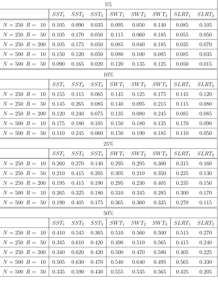
Based on the constrained and/or unconstrained SMLM estimates, Table 1 reports the re-sults of the testing that no contemporary relationships are present in the five-period three-alternative probit model. Thereby, the frequency of rejections of the null hypothesis H0 :

ln ˙ση1 = ln

³

1+ ˙corr(ηi1t,ηi2t)

1−corr˙ (ηi1t,ηi2t)

´

= 0 is displayed at the given significance levels 5%, 10%, 25%, and 50%. The unconstrained SMLM estimation refers to the flexible MMPM, whereas the constrained SMLM estimation disregards the contemporary correlations. Since the validity of H0 is first considered, the DGP is characterized by autoregressive and time invariant

relationships in the stochastic model components, but not by contemporary correlations. Overall, Table 1 reports heterogenous test results. The frequency of incorrect rejections of the null hypothesis is often noticeably higher or lower than the given significance levels. Only by using the simulated Wald test statistic SW T2 for N = 250 observations and for R = 50

orR= 200 random draws in the GHK simulator, a relatively precise conformity between the frequencies and the basic significance levels arises. This result seems to be purely random, however. By using this test statistic, the frequency of type I errors differs sizeably from the given theoretical values when other combinations of N and R are taken (e.g. for N = 500 and R = 10 based on a significance level of 50%).

For all combinations ofN andR, the use of the simple simulated likelihood ratio test statistic

SLRT1 appears relatively robust compared to the use of other test statistics even if there

are noticeable differences between the frequencies and the underlying significance levels. But the application of SST1 and SLRT2 is much more unfavorable due to the extremely strong

deviations of the frequency of type I errors from the basic significance levels (in particular with the use of the simulated likelihood ratio test statistic SLRT2 based on a theoretical

value of 50%). But also the application of the simulated score test statistics SST2 and

SST3 proves to be hardly more favorable. With the use of SST3, the frequencies are mostly

below, and with the use of SST2, the frequencies are always above the given significance

levels. Thus, none of the considered test statistics provides accurate conformities between the frequency of type I errors and the underlying significance levels for all combinations of

N and R.

Surprisingly, neither N nor R themselves have systematic effects on the frequency of type I errors. Merely by considering special versions of the simulated classical tests, partial effects can be recognized. By using, for example, the simulated Wald test statistic SW T2, an

Table 1: Frequency of rejections of H0 : lnσ˙η1 = ln ³ 1+ ˙corr(ηi1t,ηi2t) 1−corr˙ (ηi1t,ηi2t) ´ = 0 (testing that no contemporary relationships are present, validity of H0), 200 replications of the DGP

5% SST1 SST2 SST3 SW T1 SW T2 SW T3 SLRT1 SLRT2 N = 250 R = 10 0.105 0.090 0.035 0.095 0.050 0.140 0.085 0.105 N = 250 R = 50 0.105 0.170 0.050 0.115 0.060 0.185 0.055 0.050 N = 250 R= 200 0.105 0.175 0.050 0.085 0.040 0.185 0.035 0.070 N = 500 R = 10 0.150 0.120 0.050 0.080 0.100 0.085 0.085 0.035 N = 500 R = 50 0.090 0.165 0.020 0.120 0.135 0.125 0.050 0.015 10% SST1 SST2 SST3 SW T1 SW T2 SW T3 SLRT1 SLRT2 N = 250 R = 10 0.155 0.115 0.065 0.145 0.125 0.175 0.145 0.120 N = 250 R = 50 0.145 0.265 0.085 0.140 0.095 0.215 0.115 0.080 N = 250 R= 200 0.120 0.240 0.075 0.135 0.080 0.245 0.085 0.085 N = 500 R = 10 0.175 0.180 0.105 0.150 0.180 0.125 0.170 0.090 N = 500 R = 50 0.110 0.245 0.060 0.150 0.190 0.185 0.110 0.050 25% SST1 SST2 SST3 SW T1 SW T2 SW T3 SLRT1 SLRT2 N = 250 R = 10 0.260 0.270 0.140 0.295 0.295 0.300 0.315 0.160 N = 250 R = 50 0.210 0.415 0.205 0.305 0.210 0.350 0.235 0.130 N = 250 R= 200 0.195 0.415 0.190 0.295 0.230 0.405 0.235 0.150 N = 500 R = 10 0.265 0.325 0.180 0.310 0.345 0.285 0.300 0.170 N = 500 R = 50 0.190 0.405 0.175 0.365 0.360 0.335 0.270 0.115 50% SST1 SST2 SST3 SW T1 SW T2 SW T3 SLRT1 SLRT2 N = 250 R = 10 0.410 0.545 0.365 0.510 0.560 0.500 0.515 0.270 N = 250 R = 50 0.345 0.610 0.420 0.490 0.510 0.565 0.415 0.240 N = 250 R= 200 0.340 0.620 0.420 0.500 0.470 0.580 0.405 0.225 N = 500 R = 10 0.505 0.630 0.470 0.540 0.640 0.495 0.565 0.330 N = 500 R = 50 0.335 0.590 0.430 0.555 0.535 0.565 0.425 0.205

rejected H0. When SW T3 is applied, this value mostly decreases as N grows (and R is

constant), while an increase ofR(holdingN constant) mostly delivers a rise in the frequency of type I errors. In contrast, with the use of the simulated likelihood ratio test statistic

SLRT1, the frequency of incorrectly rejected H0 mostly decreases if R rises (holding N

constant). However, neither an increase in the number N of observations nor an increase in the number R of random draws in the GHK simulator ever lead to a systematically more precise conformity between the frequency of type I errors and the underlying significance levels.

It must be pointed out that these results are connected with grave problems in the computa-tion of the test statistics. Repeatedly over the 200 replicacomputa-tions of the DGP, negative values occur in the calculation of the simulated score test statistic SST1 (in such cases, the null

hypothesis is not rejected in this study). Obviously, the estimation of the information matrix is computationally problematic when the Hessian matrix of the simulated loglikelihood func-tion is applied. Even more difficulties occur, however, in the calculafunc-tion of SLRT2. With it,

the extremely strong deviations of the frequency of type I errors from the given significance levels can be explained. Accordingly, the inclusion of the quasi maximum likelihood theory into the simulated likelihood ratio test statistic SLRT2 (contrary to the investigations of

Lee, 1999) is here very problematic. Note that also in the calculation of SLRT1 (where the

results are still relatively precise with the use of this test statistic) negative values emerge, to a much smaller extent than in the calculation of SLRT2, however.

Overall, the computational problems and the imprecise test results illustrated in Table 1 might be influenced considerably by the corresponding unstable simulated estimates of the information matrix (not displayed here) and maximal values of the simulated (constrained or unconstrained) loglikelihood function. These substantial components of the simulated classical test statistics are influenced for their part by the respective constrained or uncon-strained SMLM estimates. The analysis of these estimates (not displayed here) actually shows extreme instabilities. In particular, the estimates of the variance-covariance parame-ters have a very strong variation over the 200 replications of the DGP (see also Ziegler and Eymann, 2001, for the problem of the SMLM estimation of variance-covariance parameters in the MMPM). Thus, the stability of the underlying (constrained or unconstrained) SMLM estimations also seems to have an influence on the simulated classical testing of special MMPM.

5.1.2 Type II errors

Such substantial computational problems obviously influence also the frequency of Type II errors in the examined test problem. Based on the corresponding constrained and/or unconstrained SMLM estimates, Table 2 reports the results of the testing that no

contem-Table 2: Frequency of rejections of H0 : lnσ˙η1 = ln ³ 1+ ˙corr(ηi1t,ηi2t) 1−corr˙ (ηi1t,ηi2t) ´ = 0 (testing that no contemporary relationships are present, validity of H1), 200 replications of the DGP

5% SST1 SST2 SST3 SW T1 SW T2 SW T3 SLRT1 SLRT2 N = 250 R = 10 0.275 0.495 0.295 0.690 0.650 0.660 0.585 0.210 N = 250 R = 50 0.160 0.605 0.325 0.710 0.535 0.715 0.570 0.200 N = 250 R= 200 0.120 0.685 0.395 0.715 0.485 0.760 0.600 0.195 N = 500 R = 10 0.345 0.760 0.535 0.835 0.875 0.810 0.820 0.410 N = 500 R = 50 0.285 0.880 0.690 0.775 0.830 0.825 0.830 0.280 10% SST1 SST2 SST3 SW T1 SW T2 SW T3 SLRT1 SLRT2 N = 250 R = 10 0.320 0.640 0.395 0.755 0.740 0.730 0.680 0.295 N = 250 R = 50 0.170 0.710 0.470 0.785 0.695 0.770 0.700 0.240 N = 250 R= 200 0.130 0.760 0.505 0.785 0.630 0.825 0.670 0.225 N = 500 R = 10 0.365 0.840 0.630 0.875 0.915 0.850 0.880 0.435 N = 500 R = 50 0.305 0.930 0.770 0.825 0.875 0.855 0.905 0.315 porary relationships are present. Again, the frequency of rejections of the null hypothesis

H0 : ln ˙ση1 = ln

³

1+ ˙corr(ηi1t,ηi2t)

1−corr˙ (ηi1t,ηi2t)

´

= 0 is displayed, but now only at the given significance levels 5% and 10%. Since the validity of the alternative hypothesis H1 is considered here,

the DGP of the five-period three-alternative probit model is characterized by contemporary, time invariant and autoregressive correlations in the stochastic model components.

The gravest difficulties emerge again in the calculation of the simulated score test statistic

SST1 and the simulated likelihood ratio test statistic SLRT2. Through the repeated

oc-currence of negative values, the highest frequency of type II errors results from the use of these two test statistics. In contrast, the computation of the other test statistics is more robust (only the calculation ofSLRT1 leads to very few negative values). In the comparison

between the different versions of the simulated classical tests, Table 2 reports with the use of the test statistics SST2,SW T1,SW T2,SW T3, andSLRT1 for all combinations ofN and

R comparatively low frequencies of type II errors. Overall, the use of SST2 for N = 500

observations and R = 50 random draws in the GHK simulator provides the smallest value. On the other hand, the frequency of type II errors is higher without exception when SST3 is

used. Thus, the inclusion of the quasi maximum likelihood theory (here into the simulated score test) proves again unfavorable.

Some high frequencies of type II errors might again be influenced by the instability of the simulated estimates (not displayed here) of the information matrix as well as by the het-erogenous maximal values of the simulated loglikelihood function. Thus, the relatively stable simulated estimations of the information matrix derived with the unconstrained SMLM es-timates could have an influence on the partly low frequency of type II errors in the use of all simulated Wald test statistics. In contrast, within the framework of the (misspecified) constrained SMLM estimation, the simulated estimations of the information matrix are com-paratively more unstable. For this reason, the higher frequency of type II errors with the use of the simulated score test statistics SST1 and SST3 can be explained (an exception is,

however, the use of SST2 for high N or high R). This result is remarkable because in the

framework of the testing that no autoregressive correlations are present (see section 5.2.2), the application of the different simulated score test statistics provides without exception a smaller frequency of type II errors.

Another important result in Table 2 is the clear effect of an increase in the number N of observations. As N grows (holding R = 10 or R = 50 constant), the frequency of type II errors is (often substantially) reduced in the framework of the testing that no contemporary relationships are present. This result holds for all considered simulated classical tests. In contrast, again no systematic effects of the numberRof random draws in the GHK simulator arise. On the one hand, an increase of R (holding N constant) always leads to a rise in the frequency of correct rejections of the null hypothesis whenSST2,SST3, andSW T3 are used.

On the other hand, such an increase results without exception in a rise in the frequency of type I errors when SST1,SW T2, and SLRT2 are used.

5.2

Testing that no autoregressive correlations are present

5.2.1 Type I errors

Based on the constrained and/or unconstrained SMLM estimates, Table 3 reports the re-sults of the testing that no autoregressive correlations are present. The table displays the frequency of rejections of the null hypothesis H0 : ln

³ 1+ ˙ρ1 1−ρ˙1 ´ = ln³1+ ˙ρ2 1−ρ˙2 ´

= 0 at the given sig-nificance levels 5%, 10%, 25%, and 50%. The unconstrained SMLM estimation takes place in the flexible five-period three-alternative probit model, whereas the constrained SMLM estimation disregards the autoregressive relationships. Since the validity of H0 is first

con-sidered, the DGP is characterized by contemporary and time invariant relationships in the stochastic model components, but not by autoregressive correlations.

Table 3: Frequency of rejections of H0 : ln ³ 1+ ˙ρ1 1−ρ˙1 ´ = ln³1+ ˙ρ2 1−ρ˙2 ´

= 0 (testing that no autore-gressive correlations are present, validity of H0), 200 replications of the DGP

5% SST1 SST2 SST3 SW T1 SW T2 SW T3 SLRT1 SLRT2 N = 250 R = 10 0.075 0.060 0.035 0.015 0.025 0.065 0.015 0.065 N = 250 R = 50 0.080 0.060 0.030 0.035 0.025 0.040 0.035 0.045 N = 250 R= 200 0.090 0.055 0.020 0.030 0.020 0.055 0.035 0.050 N = 500 R = 10 0.125 0.055 0.045 0.040 0.035 0.060 0.060 0.050 N = 500 R = 50 0.075 0.080 0.055 0.045 0.045 0.065 0.070 0.065 10% SST1 SST2 SST3 SW T1 SW T2 SW T3 SLRT1 SLRT2 N = 250 R = 10 0.145 0.115 0.080 0.075 0.060 0.095 0.110 0.110 N = 250 R = 50 0.140 0.110 0.070 0.070 0.060 0.085 0.085 0.090 N = 250 R= 200 0.130 0.105 0.070 0.065 0.050 0.090 0.065 0.100 N = 500 R = 10 0.180 0.135 0.115 0.090 0.080 0.110 0.110 0.120 N = 500 R = 50 0.145 0.130 0.105 0.090 0.065 0.110 0.105 0.110 25% SST1 SST2 SST3 SW T1 SW T2 SW T3 SLRT1 SLRT2 N = 250 R = 10 0.310 0.285 0.225 0.240 0.180 0.245 0.280 0.260 N = 250 R = 50 0.290 0.290 0.255 0.215 0.190 0.240 0.280 0.250 N = 250 R= 200 0.270 0.260 0.225 0.200 0.160 0.255 0.260 0.230 N = 500 R = 10 0.340 0.310 0.290 0.245 0.225 0.250 0.290 0.265 N = 500 R = 50 0.280 0.255 0.230 0.200 0.185 0.220 0.240 0.220 50% SST1 SST2 SST3 SW T1 SW T2 SW T3 SLRT1 SLRT2 N = 250 R = 10 0.540 0.540 0.500 0.475 0.455 0.475 0.535 0.480 N = 250 R = 50 0.520 0.535 0.485 0.465 0.450 0.490 0.500 0.470 N = 250 R= 200 0.485 0.530 0.470 0.470 0.415 0.470 0.490 0.465 N = 500 R = 10 0.540 0.535 0.500 0.465 0.480 0.460 0.515 0.470 N = 500 R = 50 0.515 0.540 0.495 0.475 0.485 0.450 0.525 0.440

Table 3 reports more stable conformities between the frequency of type I errors and the given significance levels than in the framework of the testing that no contemporary relationships are present (see Table 1). Frequently, only extremely small differences to the basic significance levels emerge, for example when the simulated score test statistics SST2 (for N = 250 and

R = 200) resp. SST3(forN = 500 andR= 50), the simulated Wald test statisticSW T3 (for

N = 250 and R = 50), or the simulated likelihood ratio test statisticSLRT2 (for N = 250

and R = 200) are used. The low instabilities in these cases might be primarily caused by the rather small number of 200 replications of the DGP.

With respect to the conformity between the frequency of type I errors and the given sig-nificance levels, no version of the simulated classical tests is clearly advantageous or disad-vantageous. Only sporadically, the use of the simulated Wald test statistic SW T2 and the

use of the simulated score test statistic SST1 (in particular for N = 500 and R = 10) lead

to stronger deviations of the frequencies from the underlying significance levels. Concerning these deviations, the use of SST2 and SST3 as well as SW T1 and SW T3 is slightly more

favorable than the use of SST1 and SW T2. Thereby, the frequencies are always below the

given significance levels when SW T1 and SW T2 are used. It should again be stressed that

the use of the simple simulated likelihood ratio test statistic SLRT1, but here also the use

of the more complex test statistic SLRT2 lead to robust results.

Apart from these findings, rare computational problems occur. Negative values emerge again with the calculation of SST1 and SLRT2 (this is also very seldom the case with the

calcula-tion of SLRT1), but to a comparatively small extent over the 200 replications of the DGP.

Thus, the derivation of these simulated classical test statistics is here clearly more robust than in the framework of the testing that no contemporary correlations are present. The comparatively strong computational stability and precise test results are probably influenced by the comparatively stable simulated estimates of the information matrix (not displayed here) and maximal values of the simulated loglikelihood function. The calculation of these components (influenced by comparatively precise constrained or unconstrained SMLM esti-mates, the estimates are not displayed here) is in particular more robust than in the pertinent derivatives in section 5.1.1.

Note that again neither the number N of observations nor the number R of random draws in the GHK simulator have systematic effects on the frequency of type I errors. Even partial effects do not occur when the several simulated classical test statistics are used (in contrast to the testing that no contemporary correlations are present in the five-period three-alternative probit model, see Table 1). In particular, N andR do not have systematic effects on the conformity between the frequency of type I errors and the basic significance levels. Concerning the effect of an increase of R, this result opposes again the investigations of Lee (1999) in the context of multiperiod binary probit models.

5.2.2 Type II errors

Based on the corresponding constrained and/or unconstrained SMLM estimates, Table 4 reports the results of the testing that no autoregressive relationships are present. Thus, the frequency of rejections of the null hypothesis H0 : ln

³ 1+ ˙ρ1 1−ρ˙1 ´ = ln³1+ ˙ρ2 1−ρ˙2 ´ = 0 over all 200 replications of the DGP is displayed again, however, only at the given significance levels 5% and 10%. In contrast to the previous analysis, the validity of the alternative hypothesis

H1 is considered now so that the DGP of the five-period three-alternative probit model

is characterized by contemporary, time invariant and autoregressive relationships in the stochastic model components.

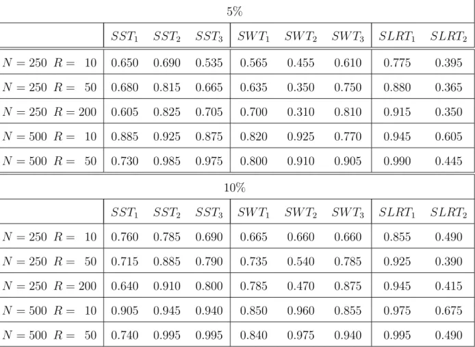
According to Table 4, the use of the simulated likelihood ratio test statistic SLRT1 is again

very favorable. In comparison with all other considered test statistics, its use delivers the smallest frequency of type II errors. This result holds for all combinations ofN and R. The use of the simulated score test statistic SST2 provides the second lowest frequencies, again

for all combinations of N and R. A somewhat higher ratio of the frequency of type II errors is derived with the use of the simulated score test statistics SST1 and SST3 as well as with

the use of all simulated Wald test statistics SW T1, SW T2, and SW T3. The use of SW T2

delivers for N = 250 a comparatively high frequency of type II errors.

Overall, however, the use ofSLRT2proves most unfavorable in this regard. Only forN = 500

andR= 10, the frequency of correct rejections ofH0 is here higher than the frequency of type

II errors. Thus, contrary to the results of Lee (1999), the inclusion of the quasi maximum likelihood theory into the simulated likelihood ratio test is again comparatively unfavorable. With the use of SLRT2, but also with the use of SST1, the type II errors over the 200

replications of the DGP are again strongly influenced by computational problems, i.e. by negative calculations of the two test statistics. Altogether, note that in the test problem considered here, the use of SLRT1 proves favorable, but the use of SST1 and in particular

the use of SLRT2 prove unfavorable. This result holds both for the precise conformity

between the frequency of type I errors and the given significance levels as well as for the small frequency of type II errors.

Despite the repeated problems in the calculation of SST1 and SLRT2, it is remarkable

that according to Table 4, lower frequencies of type II errors occur in comparison to the testing that no contemporary correlations are present (see Table 2). This result holds for all combinations of N and R. Furthermore, this result also holds for the use of the simulated score test statistics SST2 and SST3 and for the use of the simulated likelihood ratio test

statistic SLRT1. Again, these results might be considerably influenced by the more stable

simulated estimates of the information matrix (not displayed here) and maximal values of the simulated loglikelihood function. Obviously, this leads to less computational problems

Table 4: Frequency of rejections of H0 : ln ³ 1+ ˙ρ1 1−ρ˙1 ´ = ln³1+ ˙ρ2 1−ρ˙2 ´

= 0 (testing that no autore-gressive correlations are present, validity of H1), 200 replications of the DGP

5% SST1 SST2 SST3 SW T1 SW T2 SW T3 SLRT1 SLRT2 N = 250 R = 10 0.650 0.690 0.535 0.565 0.455 0.610 0.775 0.395 N = 250 R = 50 0.680 0.815 0.665 0.635 0.350 0.750 0.880 0.365 N = 250 R= 200 0.605 0.825 0.705 0.700 0.310 0.810 0.915 0.350 N = 500 R = 10 0.885 0.925 0.875 0.820 0.925 0.770 0.945 0.605 N = 500 R = 50 0.730 0.985 0.975 0.800 0.910 0.905 0.990 0.445 10% SST1 SST2 SST3 SW T1 SW T2 SW T3 SLRT1 SLRT2 N = 250 R = 10 0.760 0.785 0.690 0.665 0.660 0.660 0.855 0.490 N = 250 R = 50 0.715 0.885 0.790 0.735 0.540 0.785 0.925 0.390 N = 250 R= 200 0.640 0.910 0.800 0.785 0.470 0.875 0.945 0.415 N = 500 R = 10 0.905 0.945 0.940 0.850 0.960 0.855 0.975 0.675 N = 500 R = 50 0.740 0.995 0.995 0.840 0.975 0.940 0.995 0.490 in the calculation of SST1 and SLRT2 and, furthermore, to a higher frequency of correct

rejections ofH0 for all versions of the simulated score and the simulated likelihood ratio test

statistics.

In contrast, concerning the frequency of type II errors, no systematic differences occur be-tween the results in Table 4 and the corresponding results in Table 2 when the three simulated Wald test statistics SW T1, SW T2, and SW T3 are used. But this finding is not surprising

after the previous discussion. The stability of the underlying constrained or unconstrained SMLM estimation obviously has a relevant influence on the stability of the simulated esti-mations of the information matrix (derived with the corresponding SMLM estimates) and, thus, on the resulting frequency of type II errors. The derivative of the simulated Wald test statistics both in the testing that no contemporary correlations are present and in the testing that no autoregressive correlations are present depends itself (when the alternative hypothesis is valid) on the same unconstrained SMLM estimates in the flexible five-period three-alternative probit model.

sub-stantial influence. A rise of N (holding R = 10 or R = 50 constant) always leads to a decrease in the frequency of type II errors. This result holds for all considered test statistics. In contrast, an increase in the number R of random draws in the GHK simulator (holding

N constant) provides no clear effects. On the one hand, the frequency of type II errors decreases in this case when the simulated score test statisticsSST2 andSST3, the simulated

Wald test statistic SW T3, or the simulated likelihood ratio test statistic SLRT1 are used.

On the other hand, a rise of R (holding N constant) delivers decreases as well as increases in the frequency of type II errors when the other simulated classical test statistics are used.

6

Summary and conclusions

The Monte Carlo experiments analyzed in this paper show that the simulated classical testing in the MMPM can lead to instabilities. Thus, in the considered test problems, partly strong deviations of the frequency of type I errors from the given significance levels are present as well as high frequencies of type II errors. Note again that in each case, the number of replications of the DGP is only 200. Probably, many of the instabilities can be explained by this rather small number. Further Monte Carlo experiments about the simulated classical testing of special MMPM with a larger number of replications of the DGP would therefore be desirable in the future. However, the focus of this paper is on the comparative analysis of different test problems and in particular on the comparison of several versions of the simulated classical tests and on the investigation of the influence of the number N of observations and the number R of random draws in the GHK simulator. Therefore, many conclusions can be drawn with 200 replications of the DGP .

For example, the result that the calculation of some simulated classical test statistics is problematic is irrespective of the number of replications of the DGP. On the one hand, the simulated score test statistic SST1 proves unfavorable because repeatedly negative values of

this test statistic arise over the 200 replications of the DGP. Obviously, the estimation of the information matrix is problematic when the Hessian matrix of the simulated loglikeli-hood function is applied. This estimate of the information matrix is a substantial element of SST1. The difficulties could have been influenced by the numerical calculation of the

second-order derivatives. It is remarkable, however, that the computation of the simulated Wald test statistic SW T1 is clearly more robust although the Hessian matrix of the

simu-lated loglikelihood function is also included in this test statistic. It seems that the use of unconstrained SMLM estimates in the context ofSW T1 in contrast to the use of constrained

SMLM estimates in the context of SST1 is a computationally stabilizing factor.

But in particular, the calculation of SLRT2 is also very problematic. Thus, the inclusion of

unfavorable. With respect to this test statistic, this outcome in the MMPM considered in the present study contradicts the results of Lee (1999) in multiperiod binary probit models. Concerning the practical use ofSLRT2, note also that the implementation of this test statistic

is very complex. A comparison between the simulated score test statistics SST2 and SST3

and the simulated Wald test statisticsSW T1,SW T2, and SW T3 shows that no test statistic

is generally favorable. It should be stressed that (again in contrast to the results of Lee, 1999) the inclusion of the quasi maximum likelihood theory into the simulated score test or into the simulated Wald test is not systematically superior. This result could be related to the fact that the test statistics SST3, SW T3, and SLRT2 contain the Hessian matrix of

the simulated loglikelihood function as elements. Thus, instabilities are possible due to the numerical calculation of the second-order derivatives.

At large, the most favorable test statistic is the simple simulated likelihood ratio test statistic

SLRT1. Both in the testing that no contemporary correlations and in the testing that no

autoregressive relationships are present in the MMPM, comparatively robust test results emerge (despite sporadically occurring computational problems). Further own analyses (not displayed here) have shown that in the framework of a one-period four-alternative probit model, the use of SLRT1 is even more advantageous in relation to the other simulated

classical test statistics (the test results are available on request). This outcome refers to the testing of the independent probit model (i.e. to the testing that no contemporary correlations are present in the considered one-period multinomial probit model). Thus, according to all these results, the use of SLRT1 seems to be very favorable for the empirical testing of

several variance-covariance parameters together in one- and multiperiod multinomial probit models. The practical disadvantage of the application of this simulated classical test is that both constrained and unconstrained SMLM estimations must be performed. In future investigations, it should be examined whether this test statistic that can be implemented very easily remains favorable in the framework of the testing of other multinomial probit models.

Obviously, the precision of the underlying SMLM estimates has a strong influence on the conformity between the frequency of type I errors and the basic significance levels, on the frequency of type II errors, and on the frequency of computational problems. Concerning the frequency of type II errors, with the use of all simulated score test statistics and simulated likelihood ratio test statistics, based on the more precise SMLM estimates, the null hypothesis that no autoregressive relationships are present in the MMPM is without exception more frequently correctly rejected than the null hypothesis that no contemporary correlations are present. In contrast, no systematic differences occur when the simulated Wald test statistics are used. But these test statistics are based on the same SMLM estimates in both test problems considered here.