Optimal Monetary Policy in a Liquidity Trap

NBER WORKING PAPER SERIES

OPTIMAL MONETARY POLICY IN A LIQUIDITY TRAP Gauti B. Eggertsson

Michael Woodford Working Paper9968

http://www.nber.org/papers/w9968

NATIONAL BUREAU OF ECONOMIC RESEARCH 1050 Massachusetts Avenue

Cambridge, MA 02138 September 2003

Prepared for the International Workshop on Overcoming Deflation and Revitalizing the Japanese Economy, Economic and Social Research Institute, Tokyo, September 18, 2003. Parts of this paper have previously appeared in Eggertsson andWoodford (2003). We would like to thank Tamim Bayoumi, Ben Bernanke, Robin Brooks, Michael Dotsey, Martin Feldstein, Benjamin Friedman, Stefan Gerlach, Mark Gertler, Marvin Goodfriend, Kenneth Kuttner, Maurice Obstfeld, Athanasios Orphanides, Kenneth Rogoff, David Small, Lars Svensson, Harald Uhlig, Tsutomu Watanabe, and Alex Wolman for helpful comments, and the National Science Foundation for research support through a grant to the NBER. The views expressed in this paper are those of the authors and do not necessarily represent those of the IMF or IMF policy, nor are they necessarily those of the National Bureau of Economic Research.

©2003 by Gauti B. Eggertsson and Michael Woodford. All rights reserved. Short sections of text, not to exceed two paragraphs, may be quoted without explicit permission provided that full credit, including © notice, is given to the source.

Optimal Monetary Policy in a Liquidity Trap Gauti B. Eggertsson and Michael Woodford NBER Working Paper No. 9968

September 2003 JEL No. E52

ABSTRACT

We consider the consequences for monetary policy of the zero floor for nominal interest rates. The zero bound can be a significant constraint on the ability of a central bank to combat deflation. We show, in the context of an intertemporal equilibrium model, that open-market operations, even of “unconventional” types, are ineffective if they do not change expectations about the future conduct of policy; in this sense, a “liquidity trap” is possible. Nonetheless, a credible commitment to the right sort of history-dependent policy can largely mitigate the distortions created by the zero bound. In our model, optimal policy involves a commitment to adjust interest rates so as to achieve a time-varying price-level target, when this is consistent with the zero bound. We also discuss ways in which other central-bank actions, while irrelevant apart from their effects on expectations, may help to make credible a central bank's commitment to its target, and consider implications for the policy options currently available for overcoming deflation in Japan.

Gauti B. Eggertsson

International Monetary Fund 700 19th _{Street, NW} Washington, DC 20431 [email protected] Michael Woodford Department of Economics Princeton University Princeton, NJ 08544 and NBER [email protected]

The consequences for the proper conduct of monetary policy of the existence of a lower bound of zero for overnight nominal interest rates has recently become a topic of lively interest. The relevance of this bound is nowhere more apparent than in the case of Japan, where the call rate (the overnight cash rate that is analogous to the federal funds rate in the U.S.) has been essentially at zero for most of the time since February 1999, when the policy board of the Bank of Japan decided to make it “as low as possible”. (As shown in Figure 1, the call rate has actually been at or below 50 basis points since October 1995, so that little room for further reductions in short-term nominal interest rates has existed since that time.) At the same time, growth has remained anemic in Japan over this period, and prices have continued to fall, suggesting to many observers a need for further monetary stimulus. Yet the usual remedy — lower short-term nominal interest rates — is plainly unavailable.

This has led to interest in policies that might bring about further monetary stimulus, even taking as given the BOJ’s “zero interest rate policy” (ZIRP). Since March 2001, the BOJ has supplemented the ZIRP with a policy of “quantitative easing,” in which the supply of reserves to the banking system is increased beyond the level required in order to keep the call rate at zero.1 _{But even quite vigorous expansion of the monetary base (which, as shown} in the figure, is now more than twice as large, relative to GDP, as in the early 1990s) has not as of yet been able to halt the deflation. This suggests that Japan is currently experiencing a “liquidity trap” of the kind hypothesized by Keynes (1936), though the practical possibility of such a situation continued for decades to be debated.2 _{The result is that a problem} that was long treated as a mere theoretical curiosity — the question of what, if anything, monetary policy could do to halt deflation under such circumstances — now appears to be one of urgent practical importance.

1_{See Kimura et al. (2002) for discussion of this policy, as well as an expression of doubts about its} effectiveness.

2_{Hetzel (2003) argues that there is no liquidity trap in Japan, on the ground that the public’s holdings of} M2 plus CDs remains only a little higher than an estimated demand function estimated using earlier data would have predicted; “there is no mushrooming demand indicative of a liquidity trap” (p. 32). But one should not expect to see “mushrooming demand” for money holdings on the part of the public, if the BOJ has no way of forcing the creation of additional M2. The monetary baseissubstantially higher now than a demand function estimated on data prior to 2001 would have predicted (see,e.g.,Kimura et al.,2002), and this is what the BOJ policy of “quantitative easing” requires the private sector to hold more of.

The fact that the federal funds rate has now been reduced to only one percent in the U.S., while signs of recovery remain exceedingly fragile, has led many to wonder if the U.S. could not also soon find itself in a situation where interest-rate policy would no longer be available as a tool for macroeconomic stabilization. In the U.S. debate as well, there has been considerable discussion of whether open-market operations should not still be effective in increasing nominal aggregate demand even when the zero bound on interest rates is reached. Some have suggested that while open-market purchases of short-term Treasury bills should be ineffective under such a circumstance — on the ground that short-term Treasury paper and base money become nearly perfect substitutes in the portfolios of private traders once the federal funds rate falls to zero — open-market purchases of other kinds of assets (longer-maturity Treasury bonds, or even real assets), that do not promise the same state-contingent returns as money, should still stimulate aggregate demand.3 _{While Chairman Greenspan’s} congressional testimony in July 2003 has indicated that the Fed is unlikely to resort to such “unconventional” open-market operations in the near term, the question of the degree to which such operations would be more effective is an important one, especially for countries like Japan, where the risk of deflation is no longer a matter of conjecture.4

The question of how policy should be conducted when the zero bound is reached raises fundamental issues for the theory of monetary policy. Is a “liquidity trap” really possible, in the sense of a situation in which there is really nothing that the central bank can do to increase aggregate nominal spending or prevent continuing deflation? If monetary policy can instead be effective even when the zero bound has been reached, does its effectiveness depend on a resort to “unconventional” forms of open-market operations? And to what extent is the optimal conduct of policy different than it would be if the zero bound were never a binding constraint?

Here we seek to shed light on these issues by considering the consequences of the zero lower

3_{See,e.g.,Bernanke (2002), Cecchetti (2003), and Clouseet al. (2003).}

4_{For example, Meltzer (2003) argues that “quantitative easing” was ineffective in Japan until the BOJ} began purchasing longer-term JGBs, but attributes the recent increase in Japanese real growth to a policy of money-financed bond purchases.

1992 1994 1996 1998 2000 2002 1 1.2 1.4 1.6 1.8 2 2.2 Monetary Base/GDP 1992 1994 1996 1998 2000 2002 0 2 4 6 8 10 Call Rate

Figure 1: Evolution of the call rate on uncollateralized overnight loans in Japan, and the Japanese monetary base relative to GDP [1992 = 1.0].

bound on nominal interest rates for the optimal conduct of monetary policy, in the context of an explicit intertemporal equilibrium model of the monetary transmission mechanism. While our model remains an extremely simple one, we believe that it can help to clarify basic issues. We are able to consider the extent to which the zero bound represents a genuine constraint on attainable equilibrium paths for inflation and real activity, and to consider the extent to which open-market purchases of various kinds of assets by the central bank can mitigate that constraint. We are also able to show how the character of optimal monetary policy changes as a result of the existence of the zero bound, relative to the policy rules that would be judged optimal in the absence of such a bound, or in the case of real disturbances small enough for the bound never to matter under an optimal policy.

con-straint on what monetary stabilization policy can achieve, at least when certain kinds of real disturbances are encountered in an environment of low inflation. We argue that the possibil-ity of expansion of the monetary base through central-bank purchases of a variety of types of assets does little if anything to expand the set of feasible equilibrium paths for inflation and real activity that are consistent with equilibrium under some (fully credible) policy com-mitment. Hence the relevant tradeoffs can correctly be studied by simply considering what can be achieved by alternative anticipated state-contingent paths of the short-term nominal interest rate, taking into account the constraint that this quantity must be non-negative at all times. When we consider such a problem, we find that the zero interest-rate bound can indeed be temporarily binding, and in such a case it inevitably results in lower welfare than could be achieved in the absence of such a constraint.5

Nonetheless, we argue that the extent to which this constraint restricts possible stabiliza-tion outcomes under sound policy is much more modest than is presumed by the deflastabiliza-tion pessimists who have been widely quoted in the U.S. and European financial press in recent months. Even though the set of feasible equilibrium outcomes corresponds to those that can be achieved through alternative interest-rate policies, monetary policy is far from powerless to mitigate the contractionary effects of the kind of disturbances that would make the zero bound a binding constraint. The key to dealing with this sort of situation in the least dam-aging way is to create the right kind of expectations regarding the way in which monetary policy will be usedsubsequently,at a time when the central bank again has room to maneu-ver. We use our intertemporal equilibrium model to characterize the kind of expectations

5_{We do not here explore the possibility of relaxing the constraint by taxing money balances, as originally} proposed by Gesell (1929) and Keynes (1936), and more recently by Buiter and Panigirtzoglou (1999) and Goodfriend (2000). While this represents a solution to the problem in theory, there are substantial practical difficulties with such a proposal, not least the political opposition that such an institutional change would be likely to generate. Our consideration of the optimal policy problem also abstracts from the availability of fiscal instruments such as the time-varying tax policy recommended by Feldstein (2002). We agree with Feldstein that there is a particularly good case for state-contingent fiscal policy as a way of dealing with a liquidity trap, even if fiscal policy is not a very useful tool for stabilization policy more generally. Nonetheless, we consider here only the problem of the proper conduct of monetary policy, taking as given the structure of tax distortions. As long as one does not think that state-contingent fiscal policy can (or will) be used to eliminate even temporary declines in the natural rate of interest below zero, the problem for monetary policy that we consider here remains relevant.

regarding future policy that it would be desirable to create, and discuss a form of price-level targeting rule that — if credibly committed to by the central bank — should bring about the constrained-optimal equilibrium. We also discuss, more informally, ways in which other types of policy actions could help to increase the credibility of the central bank’s announced commitment to this kind of future policy.

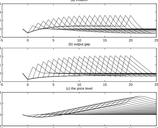
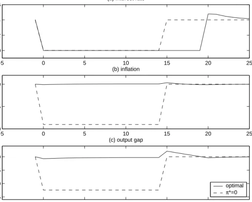
Our analysis will be recognized as a development of several key themes of Paul Krug-man’s (1998) treatment of the same topic. Like Krugman, we give particular emphasis to the role of expectations regarding future policy in determining the severity of the distortions that result from hitting the zero bound. Our primary contribution, relative to Krugman’s earlier treatment, will be the presentation of a more fully dynamic analysis. For example, our assumption of staggered pricing, rather than the simple hypothesis of prices that are fixed for one period as in the analysis of Krugman, allows for richer (and at least somewhat more realistic) dynamic responses to disturbances. In our model, unlike Krugman’s, a real distur-bance that lowers the natural rate of interest can cause output to remain below potential for years (as shown in Figure 2 below), rather than only for a single “period”, even when the average frequency of price adjustments is more than once per year. These richer dynamics are also important for a realistic discussion of the kind of policy commitment that can help to reduce economic contraction during a “liquidity trap”. In our model, a commitment to create subsequent inflation involves a commitment to keep interest rates low for a time in the future, whereas in Krugman’s model, a commitment to a higher future price level does not involve any reduction in future nominal interest rates. We are also better able to discuss questions such as how the creation of inflationary expectations during the period that the zero bound is binding can be reconciled with maintaining the credibility of the central bank’s commitment to long-run price stability.

Our dynamic analysis also allows us to further clarify the several ways in which the management of private-sector expectations by the central bank can be expected to mitigate the effects of the zero bound. Krugman emphasizes the fact that increased expectations of inflation can lower the real interest rate implied by a zero nominal interest rate. This

might suggest, however, that the central bank can affect the economy only insofar as it affects expectations regarding a variable that it cannot influence except quite indirectly; and it might also suggest that the only expectations that should matter are those regarding inflation over the relatively short horizon corresponding to the short-term nominal interest rate that has fallen to zero. Such interpretations easily lead to skepticism about the practical effectiveness of the expectational channel, especially if inflation is regarded as being relatively “sticky” in the short run. Our model is instead one in which expectations affect aggregate demand through several channels. First of all, it is not merely short-term real interest rates that matter for current aggregate demand; our model of intertemporal substitution in spending implies that the entire expected future path of short real rates should matter, or alternatively that very long real rates should matter.6 _{This means that the creation of} inflation expectations, even with regard to inflation that should occur only more than a year in the future, should also be highly relevant to aggregate demand, as long as it is not accompanied by correspondingly higher expected future nominal interest rates. Furthermore, the expected future path of nominal interest rates matters, and not just their current level, so that a commitment to keep nominal interest rates low for a longer period of time should stimulate aggregate demand, even when current rates cannot be further lowered, and even under the hypothesis that inflation expectations would remain unaffected. Since the central bank can clearly control the future path of short-term nominal interest rates if it has the will to do so, any failure of such a commitment to be credible will not be due to skepticism about whether the central bank is able to follow through on its commitment.

The richer dynamics of our model are also important for the analysis of optimal policy. Krugman mainly addresses the question whether monetary policy is completely impotent when the zero bound binds, and argues for the possibility of increasing real activity in the

6_{In the simple model presented here, this occurs solely as a result of intertemporal substitution in private} expenditure. But there are a number of reasons to expect long rates, rather than short rates, to be the critical determinant of aggregate demand. For example, in an open-economy model, the real exchange rate becomes an important determinant of aggregate demand. But the real exchange rate should be closely linked to a very long domestic real rate of return (or alternatively, to the expected future path of short rates) as a result of interest-rate parity, together with an anchor for the expected long-term real exchange rate (coming, for example, from long-run purchasing-power parity).

“liquidity trap” by creating expectations of inflation. This conclusion in itself, however (with which we agree), does not answer the question whether, or to what extent, it should actually be desirable to create such expectations, given the well-founded reasons that the central bank should have to not prefer inflation at a later time. Nor is Krugman’s model well-suited to address such a question, insofar as it omits any reason for even an extremely high degree of subsequent inflation to be harmful. Our model with staggered pricing, instead, implies that inflation (whether anticipated or not) creates distortions, and justifies an objective function for stabilization policy that trades off inflation stabilization and output-gap stabilization in terms that are often assumed to represent actual central-bank concerns. We characterize optimal policy in such a setting, and show that it does indeed involve a commitment to history-dependent policy of a sort that should result in higher inflation expectations in response to a binding zero bound. We can also show to what extent it should be optimal to create such expectations, assuming that this is possible. We find, for example, that it is not optimal to commit to so much future inflation that the zero bound ceases to bind, even though this is one possible type of equilibrium; this is why the zero bound does remain a relevant constraint, even under an optimal policy commitment.

1

Is “Quantitative Easing” a Separate Policy

Instru-ment?

A first question that we wish to consider is whether expansion of the monetary base represents a policy instrument that should be effective in preventing deflation and associated output declines, even after overnight interest rates have fallen to zero. Specifically, we wish to consider whether a policy of “quantitative easing” like that currently followed by the Bank of Japan — conceived of as an additional aspect of policy, alongside the “zero interest-rate policy” that continues to be maintained — should help to prevent further deflation. We also wish to consider the extent to which it matters which sorts of assets may be acquired by the central bank — that is, whether “unconventional” open-market operations should be expected to be more effective than simple purchases of short-term Treasury bills, as has

often been suggested in recent discussion of U.S. policy options.

Here we consider this question in the context of an explicit intertemporal equilibrium model, in which we model both the demand for money and the role of financial assets (including the monetary base) in private-sector budget constraints. The model that we use for this purpose is more detailed in several senses than the one used in subsequent sections to characterize optimal policy, in order to make it clear that we have not excluded a role for “quantitative easing” simply by failing to model the role of money in the economy. The model is discussed in more detail in Woodford (2003, chapter 4), where the consequences of various interest-rate rules and money-growth rules are considered under the assumption that disturbances are not large enough for the zero bound to bind.

Our key result is an irrelevance proposition for open market operations in a variety of types of assets that might be acquired by the central bank, under the assumption that the open market operations do not change the expected future conduct of monetary or fiscal policy (in senses that we make precise below). It is perhaps worth stating from the start that our intention in stating such a result is not to vindicate the view that a central bank is powerless to halt a deflationary slump, and hence to absolve the Bank of Japan, for example, from any responsibility for the continuing stagnation in that country. While our proposition establishes that there is a sense in which a “liquidity trap” is possible, this does not mean that the central bank is powerless under the circumstances that we describe. Rather, the point of our result is to show that the key to effective central-bank action to combat a deflationary slump is the management of expectations. Open-market operations should be largely ineffective to the extent that they fail to change expectations regarding future policy; the conclusion that we draw is not that such actions are futile, but rather that the central bank’s actions should be chosen with a view to signalling the nature of its policy commitments, and not in order to create some sort of “direct” effects.

1.1

A Neutrality Proposition for Open-Market Operations

Our model abstracts from endogenous variations in the capital stock, and assumes perfectly flexible wages (or some other mechanism for efficient labor contracting), but assumes monop-olistic competition in goods markets, and sticky prices that are adjusted at random intervals in the way assumed by Calvo (1983), so that deflation has real effects. We assume a model in which the representative household seeks to maximize a utility function of the form

Et ∞ X T=t βT−t · u(Ct, Mt/Pt;ξt)− Z ₁ 0 v(Ht(j);ξt)dj ¸ ,

whereCtis a Dixit-Stiglitz aggregate of consumption of each of a continuum of differentiated

goods, Ct ≡ ·Z ₁ 0 ct(i) θ θ−1di ¸θ−1 θ ,

with an elasticity of substitution equal toθ >1, Mtmeasures end-of-period household money

balances,7 _P

t is the Dixit-Stiglitz price index,

Pt≡ ·Z ₁ 0 pt(i) 1−θ_di ¸ 1 1−θ (1.1) and Ht(j) is the quantity supplied of labor of typej. (Each industry j employs an

industry-specific type of labor, with its own wage wt(j).) Real balances are included in the utility

function, following Sidrauski (1967) and Brock (1974, 1975), as a proxy for the services that money balances provide in facilitating transactions.8

For each value of the disturbances ξt, u(·,·;ξt) is concave function, increasing in the first

argument, and increasing in the second for all levels of real balances up to a satiation level ¯

m(Ct;ξt). The existence of a satiation level is necessary in order for it to be possible for

the zero interest-rate bound ever to be reached; we regard Japan’s experience over the past

7_{We shall not introduce fractional-reserve banking into our model. Technically,M}

trefers to the monetary

base, and we represent households as obtaining liquidity services from holding this base, either directly or through intermediaries (not modelled).

8_{We use this approach to modelling the transactions demand for money because of its familiarity. As} shown in Woodford (2003, appendix section A.16), a cash-in-advance model leads to equilibrium conditions of essentially the same general form, and the neutrality result that we present below would hold in essentially identical form were we to model the transactions demand for money after the fashion of Lucas and Stokey (1987).

several years as having settled the theoretical debate over whether such a level of real balances exists. Unlike many papers in the literature, we do not assume additive separability of the function u between the first two arguments; this (realistic) complication allows a further channel through which money can affect aggregate demand, namely an effect of real money balances on the current marginal utility of consumption. Similarly, for each value ofξt, v(·;ξt)

is an increasing convex function. The vector of exogenous disturbancesξtmay contain several

elements, so that no assumption is made about correlation of the exogenous shifts in the functions u and v.

For simplicity we shall assume complete financial markets and no limits on borrowing against future income. As a consequence, a household faces an intertemporal budget con-straint of the form

Et ∞ X T=t Qt,T[PTCT +δTMT]≤Wt+Et ∞ X T=t Qt,T ·Z ₁ 0 ΠT(i)di+ Z ₁ 0 wT(j)HT(j)dj−T h T ¸

looking forward from any period t. Here Qt,T is the stochastic discount factor by which the

financial markets value random nominal income at date T in monetary units at date t,δt is

the opportunity cost of holding money (equal to it/(1 +it), where it is the riskless nominal

interest rate on one-period obligations purchased in period t, in the case that no interest is paid on the monetary base), Wt is the nominal value of the household’s financial wealth

(including money holdings) at the beginning of periodt, Πt(i) represents the nominal profits

(revenues in excess of the wage bill) in periodtof the supplier of goodi,wt(j) is the nominal

wage earned by labor of type j in period t, and Th

t represents the net nominal tax liabilities

of each household in period t.

Optimizing household behavior then implies the following necessary conditions for a rational-expectations equilibrium. Optimal timing of household expenditure requires that aggregate demand Yt for the composite good9 satisfy an Euler equation of the form

uc(Yt, Mt/Pt;ξt) = βEt " uc(Yt+1, Mt+1/Pt+1;ξt+1)(1 +it) Pt Pt+1 # , (1.2)

9_{For simplicity, we here abstract from government purchases of goods. Our equilibrium conditions directly} extend to the case of exogenous government purchases, as shown in Woodford (2003, chap. 4).

whereit is the riskless nominal interest rate on one-period obligations purchased in periodt.

Optimal substitution between real money balances and expenditure leads to a static first-order condition of the form

um(Yt, Mt/Pt;ξt)

uc(Yt, Mt/Pt;ξt)

= it 1 +it

,

under the assumption that zero interest is paid on the monetary base, and that preferences are such that we can exclude the possibility of a corner solution with zero money balances. If both consumption and liquidity services are normal goods, this equilibrium condition can be solved uniquely for the level of real balances L(Yt, it;ξt) that satisfy it in the case of any

positive nominal interest rate.10 _{The equilibrium relation can then equivalently be written} as a pair of inequalities

Mt

Pt

≥L(Yt, it;ξt), (1.3)

it≥0, (1.4)

together with the “complementary slackness” condition that at least one must hold with equality at any time. (Here we define L(Y,0;ξ) = ¯m(Y;ξ), the minimum level of real balances for whichum = 0, so that the functionL is continuous at i= 0.)

Household optimization similarly requires that the paths of aggregate real expenditure and the price index satisfy the bounds

∞ X T=t βT_E t[uc(YT, MT/PT;ξT)YT +um(YT, MT/PT;ξT)(MT/PT)]<∞, (1.5) lim T→∞β T_E t[uc(YT, MT/PT;ξT)DT/PT] = 0 (1.6)

looking forward from any period t, where Dt measures the total nominal value of

govern-ment liabilities (monetary base plus governgovern-ment debt) at the end of period t. under the monetary-fiscal policy regime. (Condition (1.5) is required for the existence of a well-defined intertemporal budget constraint, under the assumption that there are no limitations on households’ ability to borrow against future income, while the transversality condition (1.6)

10_{In the case that i}

t= 0, L(Yt,0;ξt) is defined as the minimum level of real balances that would satisfy

must hold if the household exhausts its intertemporal budget constraint.) Conditions (1.2) – (1.6) also suffice to imply that the representative household chooses optimal consumption and portfolio plans (including its planned holdings of money balances) given its income ex-pectations and the prices (including financial asset prices) that it faces, while making choices that are consistent with financial market clearing.

Each differentiated good i is supplied by a single monopolistically competitive producer. There are assumed to be many goods in each of an infinite number of “industries”; the goods in each industry j are produced using a type of labor that is specific to that industry, and also change their prices at the same time. Each good is produced in accordance with a common production function

yt(i) =Atf(ht(i)),

where At is an exogenous productivity factor common to all industries, and ht(i) is the

industry-specific labor hired by firm i. The representative household supplies all types of labor as well as consuming all types of goods.11

The supplier of goodisets a price for that good at which it supplies demand each period, hiring the labor inputs necessary to meet any demand that may be realized. Given the allocation of demand across goods by of households in response to firm pricing decisions, on the one hand, and the terms on which optimizing households are willing to supply each type of labor on the other, we can show that the nominal profits (sales revenues in excess of labor costs) in period t of the supplier of good i are given by a function

Π(pt(i), pjt, Pt;Yt, Mt/Pt,ξ˜t) ≡ pt(i)Yt(pt(i)/Pt)−θ

−vh(f −1_(Y

t(pjt/Pt)−θ/At);ξt)

uc(Yt, Mt/Pt;ξt)

Ptf−1(Yt(pt(i)/Pt)−θ/At),

where pjt is the common price charged by the other firms in industry j.12 (We introduce

the notation ˜ξt for the complete vector of exogenous disturbances, including variations in

11_{We might alternatively assume specialization across households in the type of labor supplied; in the} presence of perfect sharing of labor income risk across households, household decisions regarding consumption and labor supply would all be as assumed here.

12_{In equilibrium, all firms in an industry charge the same price at any time. But we must define profits} for an individual supplieriin the case of contemplated deviations from the equilibrium price.

technology as well as preferences.) If prices were fully flexible, pt(i) would be chosen each

period to maximize this function.

Instead we suppose that prices remain fixed in monetary terms for a random period of time. Following Calvo (1983), we suppose that each industry has an equal probability of reconsidering its prices each period, and let 0 < α < 1 be the fraction of industries with prices that remain unchanged each period. In any industry that revises its prices in periodt, the new pricep∗

t will be the same. This price is implicitly defined by the first-order condition

Et ( _∞ X T=t αT−tQt,TΠ1(p∗t, p∗t, PT;YT, MT/PT,ξ˜T) ) = 0. (1.7)

We note furthermore that the stochastic discount factor used to price future profit streams will be given by

Qt,T =βT−t

uc(CT, MT/PT;ξT)

uc(Ct, Mt/Pt;ξt)

. (1.8)

Finally, the definition (1.1) implies a law of motion for the aggregate price index of the form Pt = h (1−α)p∗1−θ t +αPt1−−1θ i 1 1−θ . (1.9)

Equations (1.7) and (1.9) jointly determine the evolution of prices given demand conditions, and represent the aggregate-supply block of our model.

It remains to specify the monetary and fiscal policies of the government.13 _{In order to} address the question whether “quantitative easing” represents an additional tool of policy, we shall suppose that the central bank’s operating target for the short-term nominal interest rate is determined by a feedback rule in the spirit of the Taylor rule (Taylor, 1993),

it=φ(Pt/Pt−1, Yt; ˜ξt), (1.10)

13_{It is important to note that the specification of monetary and fiscal policy in the particular way that we} propose here is not intended to suggest that either monetary or fiscal policymustbe expected to be conducted according to rules of the sort assumed here. Indeed, in later sections of this paper, we recommend policy commitments on the part of both monetary and fiscal authorities thatdo not conform to the assumptions made in this section. The point is to define what we mean by the qualification that open-market operations are irrelevant if they do not change expected future monetary or fiscal policy. In order to make sense of such a statement, we must define what it would mean for these policies to be specified in a way that prevents them from being affected by past open-market operations. The specific classes of policy rules discussed here show that our concept of “unchanged policy” is not only logically possible, but that it could correspond to a policy commitment of a fairly familiar sort, one that would represent a commitment to “sound policy” in the views of some.

where now ˜ξt may also include exogenous disturbances in addition to the ones listed above,

to which the central bank happens to respond. We shall assume that the function φ is non-negative for all values of its arguments (otherwise the policy would not be feasible, given the zero lower bound), but that there are conditions under which the rule prescribes a zero interest-rate policy. Such a rule implies that the central bank supplies the quantity of base money that happens to be demanded at the interest rate given by this formula; hence (1.10) implies a path for the monetary base, in the case that the value of φ is positive. However, under those conditions in which the value of φis zero, the policy commitment (1.10) implies only a lower bound on the monetary base that must be supplied. In these circumstances, we may ask whether it matters whether a greater or smaller quantity of base money is supplied. We shall suppose that the central bank’s policy in this regard is specified by a base-supply rule of the form

Mt=PtL(Yt, φ(Pt/Pt−1, Yt; ˜ξt);ξt)ψ(Pt/Pt−1, Yt; ˜ξt), (1.11)

where the multiplicative factor ψ satisfies (i) ψ(Pt/Pt−1, Yt; ˜ξt)≥1,

(ii) ψ(Pt/Pt−1, Yt; ˜ξt) = 1 if φ(Pt/Pt−1, Yt; ˜ξt)>0

for all values of its arguments. (Condition (ii) implies that ψ = 1 whenever it > 0.) Note

that a base-supply rule of this form is consistent with both the interest-rate operating target specified in (1.10) and the equilibrium relations (1.3) – (1.4). The use of “quantitative easing” as a policy tool can then be represented by a choice of a function ψ that is greater than 1 under some circumstances.

It remains to specify which sort of assets should be acquired (or disposed of) by the central bank when it varies the size of the monetary base. We shall suppose that the asset side of the central-bank balance sheet may include any of k different types of securities, distinguished by their state-contingent returns. At the end of periodt,the vector of nominal values of central-bank holdings of the various securities is given by Mtωtm, where ωtm is a

of the form

ωm

t =ωm(Pt/Pt−1, Yt; ˜ξt), (1.12)

where the vector-valued function ωm_{(·) has the property that its components sum to 1 for}

all possible values of its arguments. The fact that ωm_{(·) depends on the same arguments as}

φ(·) means that we allow for the possibility that the central bank changes its policy when the zero bound is binding (for example, buying assets that it would not hold at any other time); the fact that it depends on the same arguments as ψ(·) allows us to specify changes in the composition of the central-bank portfolio as a function of the particular kinds of purchases associated with “quantitative easing.”

The payoffs on these securities in each state of the world are specified by exogenously given (state-contingent) vectors at and bt and matrix Ft. A vector of asset holdings zt−1 at the end of period t−1 results in delivery to the owner of a quantity a0

tzt−1 of money, a quantity b0

tzt−1 of the consumption good, and a vector Ftzt−1 of securities that may be traded in the period t asset markets, each of which may depend on the state of the world in period t. This flexible specification allows us to treat a wide range of types of assets that may differ as to maturity, degree of indexation, and so on.14

The gross nominal returnRt(j) on thejth asset between periodst−1 andtis then given

by

Rt(j) =

at(j) +Ptbt(j) +q0tFt(·, j)

qt−1(j)

, (1.13)

whereqt is the vector of nominal asset prices in (ex-dividend) periodt trading. The absence

of arbitrage opportunities implies as usual that equilibrium asset prices must satisfy q_t0 = X T≥t+1 EtQt,T[a0T +Ptb0T] T_Y−1 s=t+1 Fs, (1.14)

where the stochastic discount factor is again given by (1.8). Under the assumption that no interest is paid on the monetary base, the nominal transfer by the central bank to the

14_{For example, securityj in periodt−1 is a one-period riskless nominal bond ifb}

t(j) andFt(·, j) are zero

in all states, while at(j)>0 is the same in all states. Securityj is instead a one-period real (or indexed)

bond ifat(j) andFt(·, j) are zero, whilebt(j)>0 is the same in all states. It is a two-period riskless nominal

pure discount bond if insteadat(j) andbt(j) are zero,Ft(i, j) = 0 for all i6=k, Ft(k, j)>0 is the same in

Treasury each period is equal to Tcb

t =R0tωtm−1Mt−1−Mt−1, (1.15) where Rt is the vector of returns defined by (1.13).

We specify fiscal policy in terms of a rule that determines the evolution of total gov-ernment liabilities Dt, here defined to be inclusive of the monetary base, as well as a rule

that specifies the composition of outstanding non-monetary liabilities (debt) among differ-ent types of securities that might be issued by the governmdiffer-ent. We shall suppose that the evolution of total government liabilities is in accordance with a rule of the form

Dt Pt =d à Dt−1 Pt−1 , Pt Pt−1 , Yt; ˜ξt ! , (1.16)

which specifies the acceptable level of real government liabilities as a function of the pre-existing level of real liabilities and various aspects of current macroeconomic conditions. This notation allows for such possibilities as an exogenously specified state-contingent target for real government liabilities as a proportion of GDP, or for the government budget deficit (inclusive of interest on the public debt) as a share of GDP, among others.

The part of total liabilities that consists of base money is specified by the base rule (1.11). We suppose, however, that the rest may be allocated among any of a set of different types of securities that may be issued by the government; for convenience, we assume that this is a subset of the set of k securities that may be purchased by the central bank. If ωf_jt indicates the share of government debt (i.e., non-monetary liabilities) at the end of period t that is of type j, then the flow government budget constraint takes the form

Dt=R0tωtf−1Bt−1−Ttcb−Tth,

where Bt ≡ Dt −Mt is the total nominal value of end-of-period non-monetary liabilities,

and Th

t is the nominal value of the primary budget surplus (taxes net of transfers, if we

abstract from government purchases). This identity can then be inverted to obtain the net tax collectionsTh

t implied by a given rule (1.16) for aggregate public liabilities; this depends

Finally, we suppose that debt management policy (i.e., the determination of the compo-sition of the government’s non-monetary liabilities at each point in time) is specified by a function

ωft =ωf(Pt/Pt−1, Yt; ˜ξt), (1.17)

specifying the shares as a function of aggregate conditions, where the vector-valued function ωf _{also has components that sum to 1 for all possible values of its arguments. Together,}

the two relations (1.16) and (1.17) complete our specification of fiscal policy, and close our model.15

We may now define a rational-expectations equilibrium as a collection of stochastic pro-cesses{p∗

t, Pt, Yt, it, qt, Mt, ωtm, Dt, ωtf}, with each endogenous variable specified as a function

of the history of exogenous disturbances to that date, that satisfy each of conditions (1.2) – (1.6) of the demand block of the model, conditions (1.7) and (1.9) of the aggregate-supply block, the asset-pricing relations (1.14), conditions (1.10) – (1.12) specifying monetary policy, and conditions (1.16) – (1.17) specifying fiscal policy each period. We then obtain the following irrelevance result for the specification of certain aspects of policy.

Proposition. The set of paths for the variables{p∗

t, Pt, Yt, it, qt, Dt}that are consistent

with the existence of a rational-expectations equilibrium are independent of the specification of the functions ψ in equation (1.11), ωm _{in equation (1.12), and ω}f _{in equation (1.17).}

The reason for this is fairly simple. The set of restrictions on the processes{p∗

t, Pt, Yt, it, qt, Dt}

implied by our model can be written in a form that does not involve the variables{Mt, ωtm, ωft},

and hence that does not involve the functions ψ, ωm_{, orω}f_.

To show this, let us first note that for all m ≥m(C;¯ ξ), u(C, m;ξ) =u(C,m(C;¯ ξ);ξ),

15_{We might, of course, allow for other types of fiscal decisions from which we abstract here — government} purchases, tax incentives, and so on — some of which may be quite relevant to dealing with a “liquidity trap.” But our concern here is solely with the question of what can be achieved by monetary policy; we introduce a minimal specification of fiscal policy only for the sake of closing our general-equilibrium model, and in order to allow discussion of the fiscal implications of possible actions by the central bank.

as additional money balances beyond the satiation level provide no further liquidity services. By differentiating this relation, we see further that uc(C, m;ξ) does not depend on the exact

value ofm either, as long asm exceeds the satiation level. It follows that in our equilibrium relations, we can replace the expression uc(Yt, Mt/Pt;ξt) by

λ(Yt, Pt/Pt−1;ξt)≡uc(Yt, L(Yt, φ(Pt/Pt−1, Yt;ξt);ξt);ξt),

using the fact that (1.3) holds with equality at all levels of real balances at whichucdepends

on the level of real balances. Hence we can write uc as a function of variables other than

Mt/Pt, without using the relation (1.11), and so in a way that is independent of the function

ψ.

We can similarly replace the expression um(Yt, Mt/Pt;ξt)(Mt/Pt) that appears in (1.5)

by

µ(Yt, Pt/Pt−1;ξt)≡um(Yt, L(Yt, φ(Pt/Pt−1, Yt;ξt);ξt);ξt)L(Yt, φ(Pt/Pt−1, Yt;ξt);ξt),

since Mt/Pt must equal L(Yt, φ(Pt/Pt−1, Yt;ξt);ξt) when real balances do not exceed the

satiation level, whileum= 0 when they do. Finally, we can express nominal profits in period

t as a function

˜

Π(pt(i), pjt, Pt;Yt, Pt/Pt−1,ξ˜t),

after substitutingλ(Yt, Pt/Pt−1;ξt) for the marginal utility of real income in the wage demand

function that is used (see Woodford, 2003, chapter 3) in deriving the profit function Π.Using these substitutions, we can write each of the equilibrium relations (1.2), (1.5), (1.6), (1.7), and (1.14) in a way that no longer makes reference to the money supply.

It then follows that in a rational-expectations equilibrium, the variables{p∗

t, Pt, Yt, it, qt, Dt}

must each period satisfy the relations λ(Yt, Pt/Pt−1;ξt) = βEt " λ(Yt+1, Pt+1/Pt;ξt+1)(1 +it) Pt Pt+1 # , (1.18) ∞ X T=t βT_E t[λ(YT, PT/PT−1;ξT)YT +µ(YT, PT/PT−1;ξT)]<∞, (1.19)

lim T→∞β T_E t[λ(YT, PT/PT−1;ξT)DT/PT] = 0, (1.20) q0 t= Pt λ(Yt, Pt/Pt−1;ξt) X T≥t+1 βT−t_E tλ(YT, PT/PT−1;ξT)[PT−1a0T +b0T] T_Y−1 s=t+1 Fs, (1.21) Et ( _∞ X T=t (αβ)T−t_λ(Y T, PT/PT−1;ξT)PT−1Π˜1(pt∗, p∗t, PT;YT, PT/PT−1,ξ˜T) ) = 0, (1.22) along with relations (1.9), (1.10), and (1.16) as before. Note that none of these equations involve the variables {Mt, ωtm, ωft}, nor do they involve the functions ψ, ωm, or ωf.

Furthermore, this is the complete set of restrictions on these variables that are required in order for them to be consistent with a rational-expectations equilibrium. For given any processes{p∗

t, Pt, Yt, it, qt, Dt}that satisfy the equations just listed in each period, the implied

path of the money supply is given by (1.11), which clearly has a solution; and this path for the money supply necessarily satisfies (1.3) and the complementary slackness condition, as a result of our assumptions about the form of the functionψ.Similarly, the implied composition of the central-bank portfolio and of the public debt at each point in time are given by (1.12) and (1.17). We then have a set of processes that satisfy all of the requirements for a rational-expectations equilibrium, and the result is established.

1.2

Discussion

This proposition implies that neither the extent to which quantitative easing is employed when the zero bound binds, nor the nature of the assets that the central bank may pur-chase through open-market operations, has any effect on whether a deflationary price-level path will represent a rational-expectations equilibrium. Hence the notion that expansions of the monetary base represent an additional tool of policy, independent of the specifica-tion of the rule for adjusting short-term nominal interest rates, is not supported by our general-equilibrium analysis of inflation and output determination. If the commitments of policymakers regarding the rule by which interest rates will be set on the one hand, and the rule which total private-sector claims on the government will be allowed to grow on the other, are fully credible, then it is only the choice of those commitments that matters. Other

aspects of policy should matter in practice, then, only insofar as they help to signal the nature of policy commitments of the kind just mentioned.

Of course, the validity of our result depends on the reasonableness of our assumptions, and these deserve further discussion. Like any economic model, ours abstracts from the complexity of actual economies in many respects. This raises the question whether we may have abstracted from features of actual economies that are crucial for a correct understanding of the issues under discussion.

Many readers may suspect that an important omission is the neglect of “portfolio-balance effects,” which play an important role in much recent discussion of the policy options that would remain available to the Fed in the event that the zero bound is reached by the federal funds rate.16 _{The idea is that a central bank should be able to lower longer-term interest} rates even when overnight rates are already at zero, through purchases of longer-maturity government bonds, shifting the composition of the public debt in the hands of the public in a way that affects the term structure of interest rates. (As it is generally admitted in such discussions that base money and very short-term Treasury securities have become near-perfect substitutes once short-term interest rates have fallen to zero, the desired effect should be achieved equally well by a shift in the maturity structure of Treasury securities held by the central bank, without any change in the monetary base, as by an open-market purchase of long bonds with newly created base money.)

There are evidently no such effects in our model, resulting either from central-bank securities purchases or debt management by the Treasury. But this is not, as some might expect, because we have simply assumed that bonds of different maturities (or for that matter, other kinds of assets that the central bank might choose to purchase instead of the shortest-maturity Treasury bills) are perfect substitutes. Our framework allows for different assets that the central bank may purchase to have different risk characteristics (different state-contingent returns), and our model of asset-market equilibrium incorporates those term premia and risk premia that are consistent with the absence of arbitrage opportunities.

Our conclusion differs from the one in the literature on portfolio-balance effects for a different reason. The classic theoretical analysis of portfolio-balance effects assumes a rep-resentative investor with mean-variance preferences. This has the implication that if the supply of assets that pay off disproportionately in certain states of the world is increased (so that the extent to which the representative investor’s portfolio pays off in those states must also increase), the relative marginal valuation of income in those particular states is reduced, resulting in a lower relative price for the assets that pay off in those states. But in our general-equilibrium asset-pricing model, there is no such effect. The marginal utility to the representative household of additional income in a given state of the world depends on the household’s consumption in that state, not on the aggregate payoff of its asset portfolio in that state. And changes in the composition of the securities in the hands of the publicdon’t

change the state-contingent consumption of the representative household — this depends on equilibrium output, and while output is endogenous, we have shown that the equilibrium relations that determine it do not involve the functionsψ, ωm_{,or ω}f_.17

Our assumption of complete financial markets and no limits on borrowing against future income may also appear extreme. However, the assumption of complete financial markets is only a convenience, allowing us to write the budget constraint of the representative household in a simple way. Even in the case of incomplete markets, each of the assets that is traded will be priced according to (1.14), where the stochastic discount factor is given by (1.8), and once again there will be a set of relations to determine output, goods prices, and asset prices that do not involveψ, ωm_,orωf_{.The absence of borrowing limits is also innocuous, at}

least in the case of a representative-household model, since in equilibrium the representative household must hold the entire net supply of financial claims on the government; as long as the fiscal rule (1.16) implies positive government liabilities at each date, then, any borrowing

17_{Our general-equilibrium analysis is in the spirit of the irrelevance proposition for open-market operations} of Wallace (1981). Wallace’s analysis is often supposed to be of little practical relevance for actual monetary policy because his model is one in which money serves only as a store of value, so that it is not possible for there to be an equilibrium in which money is dominated in rate of return by short-term Treasury securities, something that is routinely observed. However, in the case of open-market operations that are conducted at the zero bound, the liquidity services provided by money balances at the margin have fallen to zero, so that an analysis of the kind proposed by Wallace is correct.

limits that might be assumed can never bind in equilibrium. Borrowing limits can matter more in the case of a model with heterogeneous households. But in this case, the effects of open-market operations should depend not merely on which sorts of assets are purchased and which sorts of liabilities are issued to finance the purchases, but also on the way in which the central bank’s trading profits are eventually rebated to the private sector (with what delay, and how distributed across the heterogeneous households), as a result of the specification of fiscal policy. The effects will not be mechanical consequences of the change in the composition of the assets in the hands of the public, but instead will result from the fiscal transfers to which the transaction gives rise; and it is unclear how quantitatively significant such effects should be.

Indeed, leaving aside the question of whether there exists a clear theoretical foundation for the existence of portfolio-balance effects, there is not a great deal of empirical support for quantitatively significant effects. The attempt of the U.S. to separately target short-term and long-term interest rates under “Operation Twist” in the early 1960’s is generally regarded as having had a modest effect at best on the term structure.18 _{The empirical literature that has} sought to estimate the effects of changes in the composition of the public debt on relative yields has also, on the whole, found effects that are not quantitatively large when present at all.19 _{For example, Agell and Persson (1992) summarize their findings as follows: “It turned} out that these effects were rather small in magnitude, and that their numerical values were highly volatile. Thus the policy conclusion to be drawn seems to be that there is not much scope for a debt management policy aimed at systematically affecting asset yields.”

Moreover, even if one supposes that large enough changes in the composition of the portfolio of securities left in the hands of the private sector can substantially affect yields, it is not clear how relevant such an effect should be for real activity and the evolution of

18_{Okun (1963) and Modigliani and Sutch (1967) are important early discussions that reached this} conclu-sion. Meulendyke (1998) summarizes the literature, and finds that the predominant view is that the effect was minimal.

19_{Examples of studies finding either no effects or only quantitatively unimportant ones include Mogigliani} and Sutch (1967), Frankel (1985), Agell and Persson (1992), Wallace and Warner (1996), and Hess (1999). Roley (1982) and Friedman (1992) find somewhat larger effects.

goods prices. For example, Clouseet al. (2003) argue that a sufficiently large reduction in the number of long-term Treasuries in the hands of the public should be able to lower the market yield on those securities relative to short rates, owing to the fact that certain institutions will find it important to hold long-term Treasury securities even when they offer an unfavorable yield.20 _{But even if this is true, the fact that these institutions have idiosyncratic reasons} to hold long-term Treasuries — and that, in equilibrium, no one else holds any or plays any role in pricing them — means that the lower observed yield on long-term Treasuries may not correspond to any reduction in the perceived cost of long-term borrowing for other institutions. If one is able to reduce the long bond rate only by decoupling it from the rest of the structure of interest rates, and from the cost of financing long-term investment projects, it is unclear that such a reduction should do much to stimulate economic activity or to halt deflationary pressures.

Hence we are not inclined to suppose that our irrelevance proposition represents so poor an approximation to reality as to deprive it of practical relevance. Even if the effects of open-market operations under the conditions described in the proposition are not exactly zero, it seems unlikely that they should be large. In our view, it is more important to note that our irrelevance proposition depends on an assumption that interest-rate policy is specified in a way that implies that these open-market operations have no consequences for interest-rate policy, either immediately (which is trivial, since it would not be possible for them tolowercurrent interest rates, which is the only effect that would be desired),or at any subsequent date either. We have also specified fiscal policy in a way that implies that the contemplated open-market operations have no effect on the evolution of total government liabilities {Dt} either — again, neither immediately nor at any later date. While we think

that these definitions make sense, as a way of isolating the pure effects of open-market purchases of assets by the central bank from either interest-rate policy on the one hand and from fiscal policy on the other, it is important to note that someone who recommends

20_{Cecchetti (2003) similarly argues that it should be possible for the Fed to independently affect long-bond} yields if it is determined to do so, given that it can print money without limit to buy additional long-term Treasuries if necessary.

monetary expansion by the central bank may intend for this to have consequences of one or both of these other sorts.

For example, when it is argued that surely nominal aggregate demand could be stimulated by a “helicopter drop of money”, the thought experiment that is usually contemplated is not simply a change in the function ψ in our policy rule (1.11). First of all, it is typically supposed that the expansion of the money supply will be permanent. If this is the case, then the functionφ that defines interest-rate policy is also being changed, in a way that will become relevant at some future date, when the money supply no longer exceeds the satiation level.21 _{Second, the assumption that the money supply is increased through a “helicopter} drop” rather than an open-market operation implies a change in fiscal policy as well. The operation increases the value of nominal government liabilities, and it is generally at least tacitly assumed that this is a permanent increase as well. Hence the experiment that is imagined is not one that our irrelevance proposition implies should have no effect on the equilibrium path of prices.

Even more importantly, we should stress that our irrelevance result applies only given

a correct private-sector understanding of the central bank’s commitments regarding future policy, which may not be present. We have just argued that the key to lowering long-term interest rates, in a way that actually provides an incentive for increased spending, is by changing expectations regarding the likely future path of short rates, rather than through intervention in the market for long-term Treasuries. As a logical matter, this need not require any open-market purchases of long-term Treasuries at all. Nonetheless, the private sector may be uncertain about the nature of the central bank’s policy commitment, and so may scrutinize the bank’s current actions for further clues. In practice, the management

21_{This explains the apparent difference between our result and the one obtained by Auerbach and Obstfeld} (2003) in a similar model. These authors assume explicitly that an increase in the money supply while the zero bound binds carries with it the implication of a permanently higher money supply, and also that there exists a future date at which the zero bound ceases to bind, so that the higher money supply will imply a different interest-rate policy at that later date. Clouseet al. (2003) also stress that maintenance of the higher money supply until a date at which the zero bound would not otherwise bind represents one straightforward channel through which open markets operations while the zero bound is binding could have a stimulative effect, though they discuss other possible channels as well.

of private-sector expectations is an art of considerable subtlety, and shifts in the portfolio of the central bank could be of some value in making credible to the private sector the central bank’s own commitment to a particular kind of future policy, as we discuss further in section 6. “Signalling” effects of this kind are often argued to be an important reason for the effectiveness of interventions in foreign-exchange markets, and might well provide a justification for open-market policy when the zero bound binds.22

We do not wish, then, to argue that asset purchases by the central bank are necessarily pointless under the circumstances of a binding zero lower bound on short-term nominal interest rates. However, we do think it important to observe that insofar as such actions can have any effect, it is not because of any necessary or mechanical consequence of the shift in the portfolio of assets in the hands of the private sector itself. Instead, any effect of such actions must be due to the way in which they change expectations regarding future interest-rate policy, or, perhaps, the future evolution of total nominal government liabilities. In sections 6 and 7 we discuss reasons why open-market purchases by the central bank might plausibly have consequences for expectations of these types. But since it is only through effects on expectations regarding future policy that these actions can matter, we shall focus our attention on the question of what kind of commitments regarding future policy are in fact to be desired. And this question can be addressed without explicit consideration of the role of open-market operations by the central bank of any kind. Hence we shall simplify our model — abstracting from monetary frictions and the structure of government liabilities altogether — and instead consider how it is desirable for interest-rate policy to be conducted, and what kind of commitments about this policy it is desirable to make in advance.

2

How Severe a Constraint is the Zero Bound?

We turn now to the question of the way in which the existence of the zero bound restricts the degree to which a central bank’s stabilization objectives, with regard to both inflation and

22_{Clouseet al. (2003) argue that this is one important channel through which open-market operations can} be effective.

real activity, can be achieved, even under ideal policy. It follows from our discussion in the previous section that the zero bound does represent a genuine constraint. The differences among alternative policies that are relevant to the degree to which stabilization objectives are achieved having only to do with the implied evolution of short-term nominal interest rates, and the zero bound obviously constrains the ways in which this instrument can be used, though it remains to be seen how relevant this constraint may be.

Nonetheless, we shall see that it is not at all the case that there is nothing that a central bank can do to mitigate the severity of the destabilizing impact of the zero bound. The reason is that inflation and output do not depend solely upon the current level of short-term nominal interest rates, or even solely upon the history of such rates up until the current time (so that the current level of interest rates would be the only thing that could possibly changed in response to an unanticipated disturbance). The expected character of future

interest-rate policy is also a critical determinant of the degree to which the central bank achieves its stabilization objectives, and this allows an important degree of scope for policy to be improved upon, even when there is little choice about the current level of short-term interest rates.

In fact, the management of expectations is the key to successful monetary policy at all

times, and not just in those relatively unusual circumstances when the zero bound is reached. The effectiveness of monetary policy has little to do with the direct effect of changing the level of overnight interest rates, since the current cost of maintaining cash balances overnight is of fairly trivial significance for most business decisions. What actually matters is the private sector’s anticipation of the future path of short rates, as this determines equilibrium long-term interest rates, as well as equilibrium exchange rates and other asset prices — all of which are quite relevant for many current spending decisions, hence for optimal pricing behavior as well. The way in which short rates are managed matters because of the signals that it gives about the way in which the private sector can expect them to be managed in the future. But there is no reason to suppose that expectations regarding future monetary policy, and hence expectations regarding the future evolution of nominal variables more generally, should

change only insofar as the current level of overnight interest rates changes. A situation in which there is no decision to be made about the current level of overnight rates (as in Japan at present) is one which brings the question of what expectations regarding future policy one should wish to create more urgently to the fore, but this is in fact the correct way to think about sound monetary policy at all times.

Of course, there is no question to be faced about what future policy one should wish for people to expect if there is no possibility of committing oneself to a different sort of policy in the future than one would otherwise have pursued, as a result of the constraints that are currently faced (and that make desirable the change in expectations). This means that the private sector must be convinced that the central bank will not conduct policy in a way that ispurely forward-looking, i.e.,taking account at each point in time only of the possible paths that the economy could follow from that date onward. For example, we will show that it is undesirable for the central bank to pursue a certain inflation target, once the zero bound is expected no longer to prevent it from being achieved, even in the case that the pursuit of this target would be optimal if the zero bound did not exist (or would never bind under an optimal policy). The reason is that an expectation that the central bank will pursue the fixed inflation target after the zero bound ceases to bind gives people no reason to hold the kind of expectations, while the bound is binding, that would mitigate the distortions created by it. A history-dependent inflation target23 _{— if the central bank’s commitment to it can} be made credible — can instead yield a superior outcome.

But this too is an important feature of optimal policy rules more generally (see, e.g.,

Woodford, 2003, chapter 7). Hence the analytical framework and institutional arrangements used to make monetary policy need not be changed in any fundamental way in order to deal with the special problems created by a “liquidity trap”. As we explain in section 4, the optimal policy in the case of a binding zero bound can be implemented through a targeting procedure that represents a straightforward generalization of a policy that would be optimal

23_{As we shall see, it is easier to explain the nature of the optimal commitment if it is described as a} history-dependent price-level target.

even if the zero bound were expected never to bind.

2.1

Feasible Responses to Fluctuation in the Natural Rate of

In-terest

In order to characterize the way in which stabilization policy is constrained by the zero bound, we shall make use of a log-linear approximation to the structural equations of section 2, of a kind that is often employed in the literature on optimal monetary stabilization policy.24 Specifically, we shall log-linearize the structural equations of our model (except for the zero bound (1.4)) around the paths of inflation, output and interest rates associated with a zero-inflation steady state, in the absence of disturbances (ξt= 0). We choose to expand around

these particular paths because the zero-inflation steady state represents optimal policy in the absence of disturbances.25 _{In the event of small enough disturbances, optimal policy will} still involve paths in which inflation, output and interest rates are at all times close to those of the zero-inflation steady state. Hence an approximation to our equilibrium conditions that is accurate in the case of inflation, output and interest rates near those values will allow an accurate approximation to the optimal responses to disturbances in the case that the disturbances are small enough.

In the zero-inflation steady state, it is easily seen that the real rate of interest is equal to ¯

r≡β−1_{−1>0,and this is also the steady-state nominal interest rate. Hence in the case of} small enough disturbances, optimal policy will involve a nominal interest rate that is always positive, and the zero bound will not be a binding constraint. (Optimal policy in this case is characterized in the references cited in the previous paragraph.) However, we are interested in the case in which disturbances are at least occasionally large enough for the zero bound to

24_{See,e.g.,Claridaet al.,(1999) or Woodford (2003). Junget al. (2001), Sugo and Teranishi (2003), and} Adam and Billi (2003) also consider optimal policy in the presence of the zero bound in frameworks like the one used here.

25_{See Woodford (2003, chapter 7) for more detailed discussion of this point. The fact that zero inflation} is optimal, rather than mild deflation, depends on our abstracting from transactions frictions, as discussed further in footnote xx below. As shown by Woodford, a long-run inflation target of zero is optimal in this model, even when the steady-state output level associated with zero inflation is suboptimal, owing to market power.