NBER WORKING PAPER SERIES
BOND RISK PREMIA John H. Cochrane
Monika Piazzesi
Working Paper 9178
http://www.nber.org/papers/w9178
NATIONAL BUREAU OF ECONOMIC RESEARCH 1050 Massachusetts Avenue
Cambridge, MA 02138 September 2002
We thank Geert Bekaert, Michael Brandt, Lars Hansen, Bob Hodrick, Narayana Kocherlakota, Pedro Santa-Clara, Martin Schneider and many seminar participants for helpful comments. Cochrane acknowledges research support from the Graduate School of Business and from an NSF grant administered by the NBER. Updated drafts of this paper are maintained on the authors’ web pages, including color graphs. The views expressed herein are those of the authors and not necessarily those of the National Bureau of Economic Research.
© 2002 by John H. Cochrane and Monika PIazzesi. All rights reserved. Short sections of text, not to exceed two paragraphs, may be quoted without explicit permission provided that full credit, including © notice, is given to the source.
Bond Risk Premia
John H. Cochrane and Monika Piazzesi NBER Working Paper No. 9178
September 2002 JEL No. G1, E4
ABSTRACT
This paper studies time variation in expected excess bond returns. We run regressions of annual excess returns on forward rates. We find that a single factor predicts 1-year excess returns on 1-5 year maturity bonds with an R2 up to 43%. The single factor is a tent-shaped linear function of forward rates. The return forecasting factor has a clear business cycle correlation: Expected returns are high in bad times, and low in good times, and the return-forecasting factor forecasts long-run output growth. The return-forecasting factor also forecasts stock returns, suggesting a common time-varying premium for real interest rate risk. The return forecasting factor is poorly related to level, slope, and curvature movements in bond yields. Therefore, it represents a source of yield curve movement not captured by most term structure models. Though the return-forecasting factor accounts for more than 99% of the time-variation in expected excess bond returns, we find additional, very small factors that forecast equally small differences between long term bond returns, and hence statistically reject a one-factor model for expected returns.
John H. Cochrane Monika Piazzesi
Graduate School of Business Anderson Graduate School of Management
University of Chicago UCLA
1101 E. 58th St. 110 Westwood Plaza
Chicago, IL 60637 Los Angeles, CA 90095
and NBER and NBER
1
Introduction
This paper studies time-varying risk premia in the term structure of interest rates. We run regressions of one year excess returns — borrow at the one year rate, buy a long term bond, and sell it in one year — on all forward rates available at the beginning of the
period. We find R2 values as high as 43%. The forecasts are statistically significant for
all maturities, even taking into account the small sample properties of test statistics. The forecasts survive in subsamples, in real time, and across two datasets. Most importantly,
the pattern of regression coefficients is the same for all maturities. A single
“return-forecasting factor,” a single linear combination of forward rates (or yields), describes
time-variation in the expected return ofall bonds. A rise in the return-forecasting factor
implies steadily greater expected excess returns for longer maturity bonds.
This work extends Fama and Bliss’s (1987) and Campbell and Shiller’s (1991) classic
regressions. Fama and Bliss found that the spread between the n-year forward rate and
the 1-year yield predicts the 1-year excess return of then-year bond, withR2 about 15%.
Campbell and Shiller found similar results forecasting yield changes with yield spreads.
(Campbell 1995 is an excellent summary.) We more than double theR2. Wefind that the
same linear combination of forward rates predicts bond returns at all maturities, where
Fama and Bliss relate each bond’s expected excess return to a different forward spread.
Our return-forecasting factor completely drives out Fama and Bliss’s forward spread in a multiple regression. Our regressions improve on Fama and Bliss’s statistical evidence for forecastable returns, especially in small samples.
We explore extensively the macroeconomic and financial interpretation and
implica-tions of our bond return forecasts, both for their own interest and to make the forecasts more concrete and believable. Fama and Bliss (1989), Harvey (1989) and many others document that the term spreads which forecast bond returns are correlated with eco-nomic conditions and forecast output and stock returns. It is natural to see how the
return-forecasting factor behaves in these roles. We find that the return-forecasting
factor has a clear business cycle correlation. Expected excess returns are high in bad times, and low in good times. However, business cycle variables do not forecast bond
returns. The return-forecasting factor apparently reflects additional or better-measured
information. The return-forecasting factor forecasts GDP growth, but only at horizons over a year, in contrast to the yield spread which forecasts output over short horizons. Thus, we overturn the link between bond excess return forecasts and short term
(mon-etary?) output fluctuations suggested by term spreads. The return-forecasting factor
also forecasts stock returns, about as much as it would forecast the return of an 8-year duration bond. The return-forecasting factor is a bit stronger in the 1990s, when interest
rate changes were largely real, than it is in the 1970s when inflation had a strong effect
on interest rates, and the return-forecasting factor is poorly correlated with inflation. All
of this evidence points to a time-varying, business cycle related premium for holding real interest rate risk.
The return-forecasting factor also forecasts changes in short-term interest rates. The classic expectations hypothesis predicts that a forward rate higher than the short rate
should forecast a rise in the short rate. Fama and Bliss’s (1987) rejection of the expec-tations hypothesis showed that this is not true — there is no tendency for the short rate
to rise in thefirst year after we observe a high forward rate. This phenomenon is theflip
side of Fama and Bliss’s return forecasts: since the interest rate does not rise, long term
bond prices do not fall to offset their higher initial yields, so long-term bond holders make
money. Our return-forecasting factordoes forecast changes in 1-year rates. However, our
forecast is roughly speaking in the “wrong direction.” When the return-forecasting factor
signals high returns on long term bonds, it forecasts a decline in the short rate that will
raise long term bond prices, so long term bond holders make even more money than by Fama and Bliss’s mechanism.
We also relate our findings to the term structure literature in finance, especially the
“multifactor affine model” literature in which all bond yields are driven by a few factors.
The return-forecasting factor is a tent-shaped linear combination of forward rates. It is not a “curvature factor” in yields, though. Expressed as a function of yields rather than forward rates, it is curved through the 4-5 year maturity rather than curved at the short end. As a result, the return-forecasting factor is poorly related to the level, slope, and curvature factors that describe the vast bulk of moments in bond yields and that form the basis of most term structure models. Much of the variation in the return-forecasting factor is related to the small additional yield curve factors that are conventionally ignored.
In addition, most term structure models are specified and estimated at monthly or even
weekly frequency. Wefind a moving average structure in the monthly yield data, possibly
induced by measurement error, so a monthly AR(1) yield representation raised to the 12th power misses much of the one-year bond return predictability and completely misses the single-factor representation. To see the return forecasts, you must look directly at the one year horizon, or more complex time series models.
These two facts may explain why the return-forecasting factor has gone unrecognized for so long in this well-studied data, and these facts carry important implications for term
structure modeling. If you first posit a factor model for yields, estimate it on monthly
data, and then look at one year expected returns, you will completely miss excess return forecastability. To incorporate our evidence on risk premia, a yield curve model must include something like our return-forecasting factor in addition to traditional factors such as “level,” “slope,” and “curvature,” even though the return-forecasting factor does little
improve the model’sfit for yields, and it must reconcile the difference between our direct
annual forecasts and those implied by short horizon regressions.
The return-forecasting factor accounts for more than 99% of the time-variation of bond expected excess returns. However, additional very small factors forecast very small
spreads between long-term bond returns with statistical significance. These additional
factors cause a statistical rejection of a single factor model for expected returns. The additional factors correspond to small, idiosyncratic, transitory movements in bond prices or yields. These movements may represent small liquidity premia, exploitable by extreme long-short positions (such as the famous 29.5 - 30 year LTCM bond spread), or they may
The expectations hypothesis remains a workhorse in applied work in macroeconomics
andfinance. For example, central banks care a lot about interest rates — how to forecast
interest rates, how monetary policy affects long term rates through its dynamic effect on
short term rates, or how to read market interest rate and inflation expectations from the
yield curve. Yet central bank researchers routinely impose the expectations hypothesis in these exercises (Clews 2002, Scholtes 2002, Söderlind and Svensson, 1997). The European Central Bank “Monthly Bulletin” explicitly uses the expectations hypothesis to compute expected future short rates from futures (see, for example, page 13 of the August 2002 issue). The monetary VAR literature, when it does not simply ignore the information in the term structure, routinely imposes the expectations hypothesis to distinguish expected from unexpected movements in interest rates, for example Rudebusch (1998), Krueger and Kuttner (1996). Our strong evidence against the expectations hypothesis casts doubt on these and related applications.
Our single factor model is similar to the “single index” or “latent variable” models used by Hansen and Hodrick (1983) and Ferson and Gibbons (1985) to capture time-varying expected returns. Stambaugh (1988) ran regressions similar to ours of 2-6 month bond excess returns on 1-6 month forward rates. After correcting for measurement error,
Stambaugh found a pattern of coefficients similar to ours (Figure 2, page 53). Stambaugh
rejected a one or two factor representation of this forecast. Ilmanen (1995) ran regressions
of monthly excess returns on bonds in different countries on a term spread, the real
short rate, stock returns, and bond return betas. Ilmanen did not reject a one factor representation for expected international excess returns consisting of a linear combination of these variables.
2
Bond return regressions
2.1
Notation
We use the following notation for log bond prices:
p(tn) = log price of n-year discount bond at time t.
We use parentheses to distinguish maturity from exponentiation in the superscript. The log yield is yt(n)≡ − 1 np (n) t .
We write the log forward rate at timet for loans between timet+n−1andt+n as
ft(n−1→n) ≡p
(n−1)
t −p
(n)
t ,
and we write the log holding period return from buying an n-year bond at time t and
selling it as ann−1year bond at time t+ 1 as
rt(n+1) ≡p (n−1)
t+1 −p (n)
We denote excess log returns by
rxt(+1n) ≡rt(+1n) −yt(1).
We use the same letters without nindex to denote vectors across maturity, e.g.
rxt+1 = h rx(2)t rx (3) t rx (4) t rx (5) t i> .
When used as right hand variables, these vectors include an intercept, e.g.
yt= h 1 yt(1) y (2) t y (3) t y (4) t y (5) t i> , ft= h 1 yt(1) f (1→2) t f (2→3) t f (3→4) t f (4→5) t i> .
We use overbars to denote averages across maturity, e.g.
rxt+1 ≡ 1 4 5 X n=2 rx(tn+1).
2.2
Excess return forecasts
Our objective is to understand time-variation in expected excess bond returns. Hence,
we run regressions of bond excess returns at timet+1on variables at timet. The natural
right hand variables are time t bond prices, yields or forward rates. Prices, yields and
forward rates are linear functions of each other, so the forecasts are the same. We find
that forward rates produce more elegant and interpretable results. Section 3 considers
the addition of macroeconomic variables to forecast bond returns, andfinds that they do
not help. We focus on an annual horizon. We use the Fama-Bliss data (available from CRSP) of 1 through 5 year zero coupon bond prices, so we can compute annual returns directly.
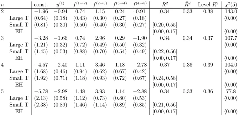
Table 1 presents regressions of excess returns on all forward rates. The top panel of
Figure 1 graphs the regression coefficients as a function of the maturity on the right hand
side — each row of Table 1 is a line of the graph. (For now, ignore the bottom panel.)
The plot makes the pattern clear — the same function of forward rates forecasts holding
period returns at all maturities. Longer maturities just have greater loadings on this same function. The pattern of coefficients suggests a common return-forecasting factor that is a tent-shaped linear combination of forward rates.
Table 1. Regressions of 1-year excess returns on all forward rates n const. y(1) f(1→2) f(2→3) f(3→4) f(4→5) R2 R¯2 Level R2 χ2(5) 2 −1.96 −0.94 0.74 1.15 0.24 -0.91 0.34 0.33 0.38 143.0 Large T (0.64) (0.18) (0.43) (0.30) (0.27) (0.18) h0.00i Small T (0.81) (0.30) (0.50) (0.40) (0.30) (0.27) [0.20,0.55] EH [0.00,0.17] h0.00i 3 −3.28 −1.66 0.74 2.96 0.29 −1.90 0.34 0.34 0.37 107.7 Large T (1.21) (0.32) (0.72) (0.49) (0.50) (0.32) h0.00i Small T (1.45) (0.53) (0.88) (0.70) (0.54) (0.49) [0.22,0.56] EH [0.00,0.17] h0.00i 4 −4.57 −2.40 1.11 3.46 1.18 −2.78 0.37 0.36 0.39 104.0 Large T (1.68) (0.46) (0.94) (0.62) (0.67) (0.42) h0.00i Small T (1.92) (0.71) (1.18) (0.93) (0.72) (0.67) [0.24,0.58] EH [0.00,0.17] h0.00i 5 −5.78 −2.98 1.48 3.93 1.14 −2.88 0.34 0.33 0.36 77.8 Large T (2.13) (0.58) (1.12) (0.73) (0.80) (0.53) h0.00i Small T (2.38) (0.89) (1.46) (1.14) (0.89) (0.85) [0.21,0.56] EH [0.00,0.17] h0.00i
NOTE: The regression equation is
rx(t+1n) =β0+β1y (1) t +β2f (1→2) t +...+β5f (4→5) t +ε (n) t+1. ¯
R2reports adjustedR2. “LevelR2” reports theR2 from a regression using the
level, not log, excess return on the left hand side,er(tn+1) −ey
(1)
t .Standard errors
are in parentheses. “Large T”standard errors use the Hansen-Hodrick GMM correction for overlap. “Small T” standard errors are based on 50,000 boot-strapped samples from an unconstrained 12 lag yield VAR. Square brackets
“[]” are 95% bootstrap confidence intervals forR2. “EH” imposes the
expec-tations hypothesis on the bootstrap: We run a 12 lag autoregression for the 1-year rate and calculate other yields as expected values of the 1-year rate.
Details are in the Appendix. “χ2”is the Wald statistic that tests whether the
slope coefficient is zero. All χ2 statistics are computed with 18 Newey-West
lags to ensure a positive definite covariance matrix. Pointed brackets “<>”
report asymptotic and bootstrapped p-values. Data source CRSP, sample 1964:1-2001:12.
The expectations hypothesis predicts coefficients of zero — nothing should forecast
bond excess returns. The regressions in Table 1 provide strong evidence against the
expectations hypothesis. The p-values for the χ2 test that all coefficients are zero are
below 1%, for all maturities. We also compute small sample distributions1 for our test
1Bekaert, Hodrick and Marshall (1997) and others have questioned the small sample properties of
1 2 3 4 5 -3 -2 -1 0 1 2 3 4
Coefficients of excess returns on forward rates
2 3 4 5 1 2 3 4 5 -3 -2 -1 0 1 2 3 4
Coefficients implied by restricted model
2 3 4 5
Figure 1: Coefficients in a regression of holding period excess returns on the one-year
yield and 4 forward rates. The top panel presents unrestricted estimates from Table 1. The bottom panel presents restricted estimates from a single-factor model reported in Table 2. The legend (2, 3, 4, 5) refers to the maturity of the bond whose excess return is forecast. The x axis gives the maturity of the forward rate on the right hand side.
statistics. To construct standard errors, we run an unrestricted 12 monthly lag vector autoregression of all 5 yields, and bootstrap the residuals. To test the expectations hypothesis (“EH” in the table), we run an unrestricted 12 monthly lag autoregression of the one year yield, bootstrap the residuals, and calculate other yields according to the expectations hypothesis. (See the Appendix for details.) Table 1 shows that the small-T standard errors are indeed slightly larger than their asymptotic counterparts.
However, inferences are not strongly affected. The small T p-values for the χ2 test still
overwhelmingly reject the expectations hypothesis.
The regressions give an impressive R2 (for excess return forecasts) of 0.34-0.37,
sug-gesting that the forecastability is economically as well as statistically important. The
R2 is consistent across maturities. One might worry that the R2 comes from the large
number of right hand variables. For reassurance, we report in Table 1 the conventional
adjusted R¯2, and it is nearly identical. However, that adjustment presumes i.i.d. data
which is not valid in this case. The point of adjusted R¯2 is to test whether the
fore-castability is spurious, and the χ2 test that the coefficients are jointly zero addresses
that issue properly. To assess sampling error and overfitting bias in R2 directly, we also
lie well above the 0.17 upper end of the 95%R2 confidence interval calculated under the expectations hypothesis.
One might worry about logs versus levels; that actual excess returns are not
fore-castable, so the coefficients in Table 1 only reflect 1/2σ2 terms and conditional
het-eroskedasticity.2 We repeated the regressions using actual excess returns, er(tn+1)
− ey(1)t
on the left hand side. The coefficients are nearly identical. The penultimate column of
Table 1 reports the R2 from these regressions, labeled “Level R2,” and they are in fact
slightly higher than theR2 for the regression in logs.
2.3
A single factor for expected bond returns
The beautiful pattern of coefficients in Figure 1 cries for us to describe expected excess
returns of bonds on all maturities in terms of a single factor, as follows:
rx(tn+1) =bn
³
γ0+γ1y(1)t +γ2ft(1→2)+...+γ5ft(4→5)
´
+ε(t+1n). (1)
bn andγn are not separately identified by this specification, since you can double all the
bs and halve all the γs. We normalize the coefficients by imposing that the average value
of bn is one, 1 4 5 X n=2 bn = 1.
With this normalization, we estimate (1) in two steps. First, we estimate the γ by
running the regression
1 4 5 X n=2 rx(tn+1) =γ0+γ1y (1) t +γ2f (1→2) t +...+γ5f (4→5) t + ¯εt+1. (2) rxt+1 =γ>ft+ ¯εt+1.
The second equality reminds us of the notationγ, f for corresponding6×1vectors and
the notation rx for the average (across maturities) excess return. Then, we estimate bn
by running the four regressions
rx(t+1n) =bn
¡ γ>ft
¢
+ε(t+1n), n= 2, 3, 4, 5.
(We explain in Section 6 why we use this two-step procedure rather than efficient GMM.)
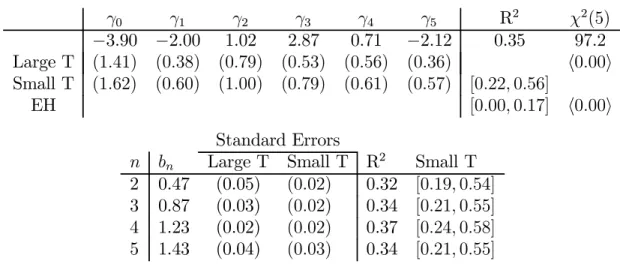
Table 2 presents the estimated values ofγ andband standard errors. Theγ estimates
are just about what one would expect from inspection of Figure 1. The loadings bn of
expected returns on the common return-forecasting factor γ>f increase smoothly with
maturity. TheR2in Table 2 are essentially the same as in Table 1. This fact indicates that
the cross-equation restrictions implied by the model (1) — that bonds of each maturity
are forecast by the same portfolio of forward rates — do little damage to the forecast
ability.
Table 2. Estimates of the return-forecasting factor.
γ0 γ1 γ2 γ3 γ4 γ5 R2 χ2(5) −3.90 −2.00 1.02 2.87 0.71 −2.12 0.35 97.2 Large T (1.41) (0.38) (0.79) (0.53) (0.56) (0.36) h0.00i Small T (1.62) (0.60) (1.00) (0.79) (0.61) (0.57) [0.22,0.56] EH [0.00,0.17] h0.00i Standard Errors
n bn Large T Small T R2 Small T
2 0.47 (0.05) (0.02) 0.32 [0.19,0.54]
3 0.87 (0.03) (0.02) 0.34 [0.21,0.55]
4 1.23 (0.02) (0.02) 0.37 [0.24,0.58]
5 1.43 (0.04) (0.03) 0.34 [0.21,0.55]
NOTE: The top panel regression is
rxt+1 =γ0+γ1y (1) t +γ2f (1→2) t +...+γ5f (4→5) t + ¯εt+1
where rxt+1 denotes the average (across maturities) excess log return. The
lower panel regression is
rx(t+1n) =bn
¡ γ>ft
¢
+ε(tn+1).
γ is the parameter estimate from the upper panel, and f denotes the vector
of all forward rates. “Large T” standard errors in the lower panel correct for
the fact that γ is estimated, by considering this estimate together with the
regression in the top panel as a single GMM estimation. “χ2” tests whether
all slope coefficients are jointly zero. Standard errors are in parentheses,
bootstrap 95% confidence intervals in square brackets “[]” and p-values angled
brackets “<>”. See notes to Table 1 for details.
The single factor model (1) is a restricted model. If we write the 4 unrestricted regressions of excess returns on all forward rates as
rxt+1 =βft+εt+1, (3)
where β is a 4×6 matrix of regression coefficients, the single factor model amounts to
the restriction
A single linear combination of forward rates γ>ft is the state variable for time-varying
expected returns of all maturities.
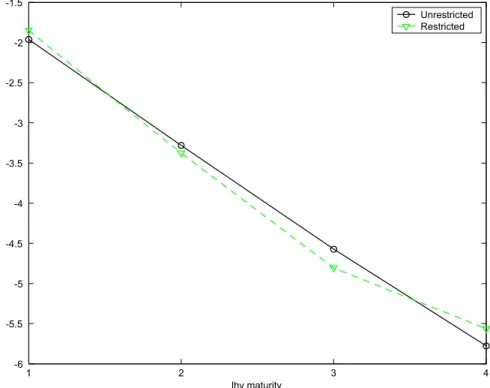
The bottom panel of Figure 1 plots the coefficients of expected returns on each of the
forward rates implied by the restricted model, i.e. for eachn, it presents£ bnγ1 · · · bnγ5
¤
. Comparing this plot with the unrestricted estimates of the top panel, you can see that the single-factor model almost exactly captures the unrestricted parameter estimates. The
specification (1) constrains the constants (bnγ0) as well as the regression coefficients
plot-ted in Figure 1. Figure 2 plots the restricplot-ted and unrestricplot-ted estimates of the constant, and you can see similarly that the estimates are very close.
1 2 3 4 -6 -5.5 -5 -4.5 -4 -3.5 -3 -2.5 -2 -1.5 lhv maturity Unrestricted Restricted
Figure 2: Restricted and unrestricted estimates of the constants. Restricted estimates
are from Table 2, and unrestricted estimates are from Table 1. Thexaxis represents the
maturity of the bond whose excess return is forecast.
The individual restricted and unrestricted estimates are close statistically as well as
economically. We could not fit standard error bounds into Figures 1 and 2, but we
computed t-statistics for the hypothesis that each parameter is individually equal to its
restricted value.3 The largestt-statistic is 0.9 and most of them are around 0.2. (Section
6 considers whether the restricted and unrestricted coefficients arejointly equal.)
3The test statistic isvec(bγ>)−vec(β)divided by the GMM standard error of unrestricted parameter
2.4
Fama-Bliss regressions
Fama and Bliss (1987) regressed each excess return against the same maturity forward
spread. This is the classic regression that providedfirst evidence against the expectations
hypothesis in this data set. Table 3 updates Fama and Bliss’s regressions to include more recent data.
Table 3. Fama-Bliss excess return regressions Maturity n α β R2 χ2(1) 2 0.04 0.94 0.14 14.2 Large T (0.30) (0.28) h0.00i Small T (0.15) (0.34) [0.01,0.35] EH [0.00,0.13] h0.02i 3 −0.14 1.24 0.14 13.5 Large T (0.54) (0.38) h0.00i Small T (0.31) (0.44) [0.01,0.36] EH [0.00,0.14] h0.02i 4 −0.41 1.50 0.15 11.6 Large T (0.76) (0.50) h0.00i Small T (0.45) (0.51) [0.01,0.38] EH [0.00,0.14] h0.03i 5 −0.11 1.10 0.06 3.7 Large T (1.05) (0.62) h0.11i Small T (0.59) (0.70) [0.00,0.28] EH [0.00,0.14] h0.20i
NOTE: The regressions are
rx(tn+1) =α+β³ft(n−1→n)−y
(1)
t
´
+ε(t+1n).
Standard errors are in parentheses, bootstrap 95% confidence intervals in
square brackets “[]” and p-values angled brackets “<>”. See notes to Table
1 for details.
The expectations hypothesis predicts a coefficient of zero. Instead, Table 3 shows
that the forward spread moves essentially one-for-one with expected excess returns on long term bonds. Fama and Bliss’s regressions have held up well since publication, unlike many other anomalies.
The multiple regressions in Table 1 and the single factor model in Table 2 provide stronger evidence against the expectations hypothesis than do the updated Fama-Bliss regressions in Table 3 in many respects. For 3 of the 4 bonds, the Fama-Bliss regressions
forecast excess returns with statistical significance, whether using asymptotic or
boot-strap confidence intervals and p-values.4 Tables 1 and 2 show strongerχ2 rejections, and
do so for all maturities. They more than double Fama and Bliss’s R2 from below 0.15
in Table 3 to 0.34-0.37 in Tables 1 and 2. The 5-year rate R2 is particularly dramatic,
jumping from 0.06 in Table 3 to 0.34 in Table 1. In the Fama-Bliss regressions, 3 of the
4 bonds show R2 just above the 95% confidence interval, mirroring the narrow, but still
significant statistical rejections. The R2 in Tables 1and 2 are nearly double the upper
end of their expectations hypothesis confidence intervals. The 0.20-0.24 lower end of the
R2 confidence intervals in Table 1 lie above the0.15R2 of the Fama- Bliss regression.
If the return-forecasting factor really is an improvement, it should drive out other
variables, and the Fama-Bliss spread in particular. The individual coefficient standard
errors in Table 1 already suggest that the additional right hand variables are important. Table 4 presents multiple regressions contrasting the single factor model of Table 2 with the Fama-Bliss regressions.
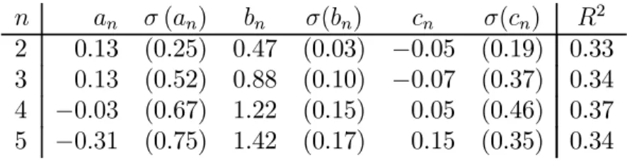
Table 4. Contest betweenγ>f and Fama-Bliss
n an σ(an) bn σ(bn) cn σ(cn) R2
2 0.13 (0.25) 0.47 (0.03) −0.05 (0.19) 0.33
3 0.13 (0.52) 0.88 (0.10) −0.07 (0.37) 0.34
4 −0.03 (0.67) 1.22 (0.15) 0.05 (0.46) 0.37
5 −0.31 (0.75) 1.42 (0.17) 0.15 (0.35) 0.34
NOTE: Multiple regression of excess holding period returns on the return-forecasting factor and Fama-Bliss slope. The regression is
rx(tn+1) =an+bn ¡ γ>ft ¢ +cn ³ ft(n−1→n)−y (1) t ´ +ε(tn+1).
Standard errors in parentheses use the Hansen-Hodrick GMM correction for overlap.
In the presence of the Fama-Bliss forward spread, the coefficients and significance
of the return-forecasting factor from Table 2 are unchanged in Table 4. The R2 is also
unaffected, meaning that the addition of the Fama-Bliss forward spread does not help to
forecast bond returns. On the other hand, in the presence of the return-forecasting factor,
the Fama-Bliss slope is destroyed as a forecasting variable. The coefficients decline from 1
or even more to almost exactly zero, and are insignificant. Clearly, the return-forecasting
factor subsumes all the predictability of bond returns captured by the Fama-Bliss forward spread.
4We useχ2 rather than a t test as we reportχ2 tests that multiple parameters are jointly zero in
other tables. The χ2 values are not squared t statistics, because we use Hansen-Hodrick weights to
compute individual standard errors, but Newey-West weights with more lags to compute χ2 statistics.
Newey-West weights are necessary to ensure positive definite covariance matrices in tests of multiple parameters.
The most important comparison is economic, not statistical. The single factor model
of Table 2 describes expected excess returns on all bonds with a single state variable,
γ>f
t. The Fama-Bliss regressions describe the expected return of each bond with a
separate state variable, its own forward spread. It is a much more useful specification to think of a common element to expected returns, at least across a range of maturities.
This comparison is not a criticism of Fama and Bliss. The Fama-Bliss specification
is exactly right for Fama and Bliss’s purpose. They wanted to explore the expectations hypothesis and, eventually, to reject it. The individual forward spreads have important interpretations in the expectations hypothesis, so they are natural right hand variables
if one is guided by that null. Our purpose is different. We want to characterize expected
excess returns, knowing the expectations hypothesis is false. The multiple regression is
a more natural specification when we are guided by that null, and it’s not surprising in
retrospect that it works better for its purpose.
2.5
Short rate forecast
Fama and Bliss also regressed changes in the 1-year rate on forward spreads. Short rate forecasts and excess return forecasts are mechanically linked, but seeing the same phe-nomenon as a short rate forecast provides a useful complementary intuition and suggests many additional implications.
Here, the expectations hypothesis predicts a coefficient of 1.0 — if the forward rate
increases one percentage point over the short rate, we should see the short rate rise one percentage point on average. Corresponding to the expectations hypothesis failure in Table 4, the Fama Bliss regression in Table 5 shows that the 2-year forward rate has no
power to forecast a 1-year change in the 1-year rate. The coefficient is essentially zero,
and one fourth of a standard error away from zero. Under the expectations hypothesis
null the R2 confidence interval is from 7 to 32% — short rates should be predictable,
given there is variation in the forward spread. Yet theR2 is zero, and the test for a zero
coefficient passes at a 98% probability value.
The unconstrained regression in Table 5 again contrasts strongly with the Fama-Bliss regression. All the forward rates taken together have substantial power to predict
one-year changes in the short rate. The R2 for short rate changes jumps to a substantial
23%. The χ2 test strongly rejects the null that the parameters are jointly zero.
This forecastability of the short rate does not revive the expectations hypothesis. Instead, the short rate becomes forecastable precisely because the expectations hypothesis is even more wrong than Fama and Bliss suspected. To understand this claim, suppose the forward spread rises one percentage point, so long term bond yields are higher than the 1-year rate. According to the expectations hypothesis, the 1-year rate is expected
to rise one percentage point. This rise will lower prices of long term bonds, offsetting
their now higher yields and generating no change in expected return. In Fama and Bliss’s regressions, the 1-year rate moves sluggishly. When the forward spread is high,
the offsetting rise in 1-year rates does not materialize for a few years, so long term bond holders make an extra return from the higher yield of long term bonds. In the regressions of Tables 1 and 2, we see much larger variation in the expected excess return. Fama and Bliss’s mechanism has been exhausted. To generate larger expected returns, we must be able to forecast short rate movements, roughly speaking in the “wrong” direction. If our
regression forecasts a 2% excess return on long term bonds, it must predict a decline in
short rates, which will raise long term bond prices.
Table 5. Predicting short rate changes
const. ft(1→2)−y (1) t y (1) t f (1→2) t f (2→3) t f (3→4) t f (4→5) t R2 χ2 Fama-Bliss -0.04 0.06 0.00 0.1 Large T (0.30) (0.28) <0.98> EH [0.07,0.32] <1.00> Unconstrained 1.96 −0.06 0.26 −1.15 −0.24 0.91 0.23 118.5 Large T (0.64) (0.18) (0.43) (0.30) (0.27) (0.18) Small T (0.82) (0.30) (0.50) (0.40) (0.30) (0.27) [0.16,0.41] h0.00i EH [0.08,0.35] h0.00i
NOTE: The Fama-Bliss regression is
y(1)t+1−y(1)t =β0+β1
³
ft(1→2)−yt(1)´+εt+1. The unconstrained regression equation is
y(1)t+1−y(1)t =β0+β1y (1) t +β2f (1→2) t +...+β5f (4→5) t +εt+1.
χ2 tests whether all slope coefficients are jointly zero (5 degrees of freedom
unconstrained, one degree of freedom for Fama-Bliss). Standard errors are in
parentheses, bootstrap 95% confidence intervals in square brackets “[]” and
p-values angled brackets “<>”. See notes to Table 1 for details.
To see the same points more formally, start with the definition,
rx(2)t+1 =p(1)t+1−p(2)t −y (1) t =−y (1) t+1−p (2) t +p (1) t =−y (1) t+1+f (1→2) t rx(2)t+1 =³yt(1)+1−yt(1)´+³ft(1→2)−yt(1)´,
and hence, using any set of forecasting variables,
Et
³
rx(2)t+1´=Et
³
Under the expectations hypothesis, expected excess returns are constant, so any move-ment in the forward spread must be matched by movemove-ments in the expected 1-year rate change. In Fama and Bliss’s regressions, the expected yield change term is constant, so changes in the forward spread must move one for one with changes in the expected ex-cess return. In our regressions, expected returns move more than changes in the forward spread. The only way to generate such changes is if the 1-year rate becomes forecastable as well.
Equation (4) also means that the regression coefficients which forecast the 1-year rate
change in Table 5 are exactly equal to our return-forecasting factorb2γ>ftwhich forecasts
Et
³
rx(2)t+1´minus a coefficient of one on the 2-year forward spread. The same factor that
forecasts excess returns is also the state variable that forecasts the short rate.
(Fama and Bliss found that the expectations hypothesis works better over longer horizons. Though the 2 year forward rate has little power to forecast the one year change in the one year rate, the 5-year forward rate moves nearly one-for-one with the expected four-year change in the 1-year rate. This means that the 5-year forward spread does not
forecast thefour year return on 5-year bonds, though it does forecast theone-year return
on 5-year bonds. They relate this pattern to a slow moving AR(1) for the one year rate. The extension of our work to longer horizons is not straightforward, so in the interest of length we do not pursue it in this paper.)
3
Macroeconomic interpretation
What is the intuition and economic significance of the return-forecasting factor? We start
by relating the return-forecasting factor to macroeconomic variables and to stock returns. The slope of the term structure is correlated with recessions and forecasts stock returns (Fama and French 1989) and it forecasts output growth (Harvey 1989, Stock and Watson 1989, Estrella and Hardouvelis 1991, Hamilton and Kim 1999). Since we substitute the return-forecasting factor for the term structure slope in forecasting bond excess returns, we naturally want to see how it performs in these other roles.
Figure 3 presents the return-forecasting factor together with the unemployment rate and the NBER peaks and troughs. The return-forecasting factor is closely associated with business cycles. Expected returns are high in bad times and low in good times. The return-forecasting factor is a “level” variable rather than a “growth” variable. It is high
when the level of unemployment is high, or the level of income is low, rather than being
high during recessions defined as periods of poor GDP growth. Campbell and Cochrane
(1999) model this kind of business cycle related risk premium.
The correlation between the return-forecasting factor and unemployment is also ev-ident at lower frequencies than usual business cycles. The return-forecasting factor in-creases throughout the 70s and dein-creases throughout the 80s, mirroring the unemploy-ment rate as it mirrors many measures of a two-decade-long productivity dip.
The return-forecasting factor is correlated with many other recession indicators as well, including industrial production growth, Lettau and Ludvigson’s (1999) consump-tion/wealth ratio, the investment/GDP ratio, and so on. It is much less correlated with
inflation. We present the graph for unemployment as it has the highest correlation among
the cyclical indicators we examined.
3.1
Macroeconomic forecasts of bond returns
Given the high correlation between the return factor and the unemployment rate, a nat-ural question is whether we can use unemployment or other macro variables to forecast bond excess returns, either alone or in addition to the return-forecasting factor. The
answer is no, or at least not among the variables we have tried. The fact that macro
variables by themselves do not forecast bond excess returns is an unfortunate result for economic interpretation. (This is equally true for Fama and Bliss’s 1987 or Campbell
and Shiller’s 1991 specifications). It would be much nicer if we could understand bond
expected excess returns as a simple mirror of macroeconomic conditions. It appears
instead that bond market prices reflect information beyond that available in
macroeco-nomic aggregates, and this information is crucial to forecasting bond excess returns. On the other hand, the fact that macro variables add nothing to the return-forecasting factor
1965 1970 1975 1980 1985 1990 1995 2000 -3 -2 -1 0 1 2 3 4 Return forecast Unemployment
Figure 3: Return forecasting factor γ0f
t and unemployment rate. Both series are
trans-formed to[xt−E(x)]/σ(x)so that they fit on the same graph. Shaded areas are NBER
in multiple regressions is a fortunate result for empirical analysis: it means we can stick
to the model Et(rxt+1) =γ>ft with great accuracy, even in VAR systems that include
macroeconomic variables.
Table 6 contrasts forecasting regressions of the average (across maturities) 1-year
bond excess return rxt+1 on the return-forecasting factor γ>ft, the unemployment rate
Ut, and other macroeconomic variables. The first row reminds us of the 0.35 R2 and
high t statistic when we forecast bond excess returns from γ>f
t. Despite its beautiful
correlation with the return-forecasting factor, unemployment U forecasts bond excess
returns only 0.05 R2. In a multiple regression, unemployment does not affect the size
and significance of theγ>f
tcoefficient, and only raises theR2 to0.38. The Stock-Watson
(1989) leading index XLI is designed to forecast output growth at a 6 month horizon.
Alas, it forecasts bond excess returns with an even lower R2 of 0.01 and has no effect
in a multiple regression. Lettau and Ludvigson’s (2001) consumption-wealth ratio cay,
which forecasts income growth and stock returns, does no better. Finally, CPI inflation
is just as useless as the others.
Table 6. Macro forecasts of bond excess returns
γ>f (t) U (t) XLI (t) cay (t) cpi (t) R2
1 (7.2) 0.35 0.54 (1.5) 0.05 1.19 (7.6) -0.50 (-1.6) 0.38 -0.11 (-0.6) 0.01 1.01 (6.8) -0.14 (-1.2) 0.36 0.44 (1.03) 0.02 1.01 (7.8) −0.08 (−0.2) 0.35 −0.24 (−0.84) 0.03 0.99 (7.6) -0.5 (1.6) 0.38
NOTE: Forecasts of average (across maturities) bond returns rxt+1. U =
the unemployment rate. XLI = Stock-Watson leading indicator. cay =
the Lettau-Ludvigson consumption-wealth ratio using end of period wealth.
cpi = inflation, the one-year growth in the CPI index. Overlapping annual
forecasts, 1964:01-2001:12. Standard errors in parentheses are corrected for overlap and heteroskedasticity by GMM.
It is tempting to conclude from the fact that unemployment does not forecast out-put that the “level” movement of the return-forecasting factor shown in Figure 3 is irrelevant; that only the high frequency blips matter. This would be a mistake. The return-forecasting factor could easily have chosen not to load on the level of interest
rates, producing a much flatter graph. It did not; the regression coefficients γ sum to
3.2
Term structure forecasts of output growth
The term structure slope forecasts output growth as well as bond returns. Does the
return-forecasting factor γ>f forecast output growth? Figure 4 contrasts regressions of
GDP growth using the return forecasting factor γ>f and the yield spread y(5) −y(1).
We look at GDP growth multiple periods ahead. For example, the regression using the return-forecasting factor is ln (GDP)t+x−ln(GDP)t+x−1/4 =α+β ¡ γ>ft ¢ +εt+x,
where x is the number of years ahead, plotted on the x axis of Figure 4. For horizons
out to a year, the term structure slope forecasts GDP growth well. However, the
return-forecasting factor has absolutely no power to forecast GDP growth for thefirst year.
0 0.5 1 1.5 2 2.5 3 -0.5 0 0.5 1 Coefficients γ ′ f slope 0 0.5 1 1.5 2 2.5 3 -2 0 2 4 t statistics γ ′ f slope 0 0.5 1 1.5 2 2.5 3 0 0.05 0.1 horizon, years R2 γ ′ f slope
Figure 4: Coefficients, t-statistics and R2 in long-run GDP growth forecasts. The
un-derlying regressions forecast one-quarter GDP growth x years ahead using the
return-forecasting variable γ>f and the term structure slope y(5)
−y(1). Sample is quarterly,
1964-2001.
The fact that the slope forecasts output and bond returns has long pointed to an attractive common element to these forecasts. Our regressions overturn this conclusion. The component of the yield spread that forecasts near-term output growth is uncorrelated with the component that forecasts bond excess returns, and conversely, the component (correlated with the return-forecasting factor) that forecasts bond returns does not fore-cast near-term output growth. .
For horizons beyond a year, however, the pattern changes. Now the return-forecasting factor forecasts GDP growth, while the slope has less and less power to do so. We conclude again that bond expected excess returns are “level” variable like the unemployment rate, the consumption-income ratio (Cochrane 1994) or the consumption-wealth ratio (Lettau and Ludvigson 2001) that forecasts long-term output growth, rather than a variable like
the slope that forecasts near-term growth, possibly due to short-termfinancial or
mone-tary factors. (Multiple regressions show the same pattern of coefficients andt-statistics.
A wide variety of other output forecast variables, including the consumption-wealth ratio,
the Stock-Watson leading index, etc., and other definitions of output, including industrial
production and the coincident index, lead to similar results.)
3.3
Forecasting stock returns
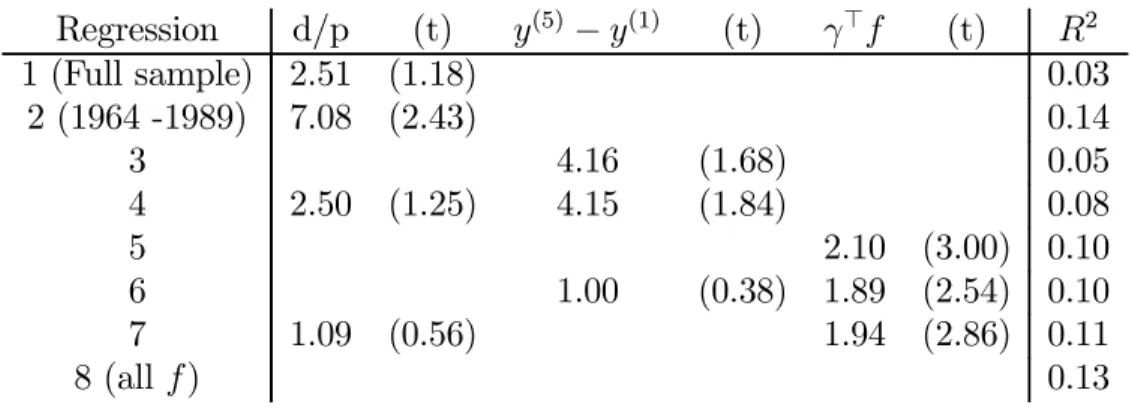
The slope of the term structure forecasts stock returns, as emphasized by Fama and French (1989). This is important evidence that the forecast corresponds to a real risk premium and not to a bond-market fad or measurement error in bond prices. We can view a stock as a long term bond plus risk; unless time-varying stock market risk premia move exactly opposite to time-varying bond market risk premia, a bond return forecasting factor should forecast stock returns much as it would a long-term bond. Table 7 evaluates how well our return-forecasting factor forecasts stock returns.
Table 7. Forecasts of excess stock returns
Regression d/p (t) y(5) −y(1) (t) γ>f (t) R2 1 (Full sample) 2.51 (1.18) 0.03 2 (1964 -1989) 7.08 (2.43) 0.14 3 4.16 (1.68) 0.05 4 2.50 (1.25) 4.15 (1.84) 0.08 5 2.10 (3.00) 0.10 6 1.00 (0.38) 1.89 (2.54) 0.10 7 1.09 (0.56) 1.94 (2.86) 0.11 8 (all f) 0.13
NOTE: The left hand variable is the one-year return on the value-weighted NYSE stock return, less the 1-year bond yield. The right hand variables are as indicated in the column headings. Overlapping monthly observations of annual returns, 1964-2001, except regression 2 from 1964-1989. The dividend price ratio is based on the return with and without dividends for the preced-ing year. T-statistics are in parentheses. Standard errors are corrected for overlap.
The first 4 regressions remind us of stock return forecastability from the dividend
the 1990s, the dividend price ratio was a strong return forecaster, with a 14% R2. The long boom of the 1990s cut down this forecastability dramatically, especially in our rather short sample (for these purposes) starting only in 1964. Of course, one good crash will restore the d/p forecastability. The term spread in the third regression forecasts the
VW stock return with a 4.2 coefficient — one percentage point term spread corresponds
to 4.2 percentage point increase in stock return. The R2 is only 5% however. The
fourth regression shows that the term spread and dividend price ratio forecast different
components of returns, since the coefficients are unchanged in multiple regressions and
theR2 increases, though to a still low 8%.
The fifth regression introduces the return-forecasting factor. It is significant, which
neither d/p (in this sample) nor the term spread are, and at 10%, itsR2 is slightly higher
than that of the term spread and d/p combined. The coefficient is 2.10. The
return-forecasting factor is the average expected return across 2-5 year bonds. The 5-year bond
in Table 2 had a coefficient of 1.43 on the return-forecasting factor, and the coefficients
rose 0.2-0.4 per year of maturity. Thus, the stock return coefficient of 2.10 is what would
expect of a bond with about 8-year duration, which is sensible. (8 year duration is also
the result of fitting a linear plus square root function of maturity to the coefficients in
Table 2.)
The sixth and seventh regressions compare the bond return-forecasting factor with
the term spread and d/p. The bond return forecasting factor’s coefficient and significance
are hardly affected in this multiple regression, while the d/p and term coefficients are cut
more than in half and rendered even less significant.
Last, we consider an unrestricted regression of stock excess returns on all forward rates. Of course, this estimate will be noisy, since stock returns are more volatile than
bond returns. All forward rates together produce anR2 of 13%, only slightly more than
the γ>f R2 of 10%. The stock return forecasting coefficients (not reported) recover a
similar tent shape pattern, though not exactly the same as those of the return-forecasting factor.
4
Finance interpretation
We now relate the return-forecasting factor to term structure models in finance. These
models decompose yield curve movements into linear combinations of yields, or “factors,”
that explain the majority of the variance of yield changes.5 Most such decompositions
find “level,” “slope,” and “curvature” factors that move the yield curve in corresponding
shapes. It is tempting to look at our tent-shaped function of forward rates, and to conclude that the return-forecasting factor is a “curvature” factor in the yield curve.
5For example, Dai and Singleton 2002 and Duffee 2002 construct affine multifactor models consistent
with Fama and Bliss’s 1987 regressions. Much effort in these models, which we do not address here, goes in to specifying short rate dynamics and market prices of risk toderive a linear factor representation for bond yields. We simply characterize the results, i.e. we examine directly the linear factor representations which affine models would spend a lot of time deriving.
This temptation is misleading, however, because our tent-shaped function is a function offorward rates, not yields. Forward rates and yields span the same bond prices of course,
so we can also express the forecasting factor as a function of yields, γ∗>y
t =γ>ft. The
forecasts are exactly the same, but the weights γ∗ are different than the weights γ.
The top of Figure 5 plots the return-forecasting factor as a function of yields. The
return-forecasting factor is curved at thelongend, not the short end of the yield curve. It
loads most strongly on the 4-5 year spread, not short spreads. To make an explicit
com-parison, the bottom of Figure 5 plots the first 3 principal components of yield changes.
We calculate these principal components from an eigenvalue decomposition of the covari-ance matrix of yield changes. (A similar factor analysis of the covaricovari-ance matrix of yield levels produces very similar results.) We label the principal components “level,” “slope,”
and “curvature” based on the shape of these loadings. As the figure shows, the
curva-ture factor is curved at the short end of the yield curve. The return-forecasting factor
is clearly not this “curvature” factor in yields, or any other of the first three principal
components. 1 2 3 4 5 -15 -10 -5 0 5 10 15 γ* 1 2 3 4 5 -0.8 -0.6 -0.4 -0.2 0 0.2 0.4 0.6 level slope curvature
Yield factor loadings
Figure 5: The top graph shows coefficientsγ∗in a regression of average (across maturities)
holding period returns on all yields, rxt+1 =γ∗>yt+εt+1. The bottom graph shows the
loadings of thefirst three principal components of yield changes labeled “level,” “slope,”
and “curvature.”
Table 8 collects facts about these principal components and comparisons with the return-forecasting factor. We dub the fourth yield factor “spreads” since it loads on the
spread between 3 and 2,5 year yields, and we dub the fifth yield factor “zigzag” for a
first row of Table 8 shows that as usual in such decompositions, the first two or three factors explain the vast majority of the variance of yield changes. The last column shows
how γ>f does in the factor model’s job — explaining variance of yield changes. γ>f
explains only 0.3% of the variance of yield changes. Not a very useful factor.
Table 8. Yield factors
Level Slope Curvature Spreads Zigzag γ>f
% ofvar(∆y) explained by this factor 93.7 4.4 0.8 0.6 0.6 0.3
% ofvar(γ>f) explained by this factor 0.5 37 0.4 42 21 100
R2 forecasting rxt+1 from this factor (%) 2.6 5.2 7.3 8.9 9.1 35.1
R2 forecasting rx
t+1 from up to this (%) 2.6 22.6 26.5 26.7 35.1
NOTE: The yield curve factors xt are formed from an eigenvalue
decomposi-tion of the covariance matrix of yield changesvar(∆y) =QΛQ>. Thefirst row
is the fraction yield change variance due to thekth factor,Λ(k, k)/PkΛ(k, k).
In theγ>f column of thefirst row, wefirst run a regression∆y(n)
t =a+bγ>ft+
εt, and then calculate 100×trace(cov(bγ>f))/trace(cov(∆y)). The second
row decomposes the variance ofγ>f into components due to each factor. We
findα inγ>f
t=α>xtand then calculate100×α(k)2Λ(k, k)2/var(γ>f). The
third row presentsR2 from forecasting regressions of the average (across
ma-turities) excess return on the factors, rxt+1 = α+βx
(k)
t +εt+1. The fourth
row presentsR2 from corresponding multiple regressionsrx
t+1 =α+β1x (1) t + ...+βkx (k) t +εt+1. Sample 1964-2001.
In the second row, we ask howγ>f is related to the yield curve factors. The loadings
(regression coefficients ofγ>f
ton the yield curve factors at timet) are not that interesting,
so we calculate the fraction of the variance ofγ>f due to each of the (orthogonal) factors
in turn. γ>f is correlated with the slope factor, so the slope factor explains the largest
fraction, 37% of γ>f variance. Curvature accounts for only 0.4% of γ>f variance - the
return-forecasting factor γ>f really does have nothing to do with the curvature factor.
The spreads factor, essentially insignificant for yields turns out to be quite significant at
42% for explaining expected returns through γ>f. The zigzag factor is also important,
explaining 21%.
The third row of Table 8 asks how well we can forecast returns using yield curve factors
in place ofγ>f. The yield curve factors individually do a poor job of forecasting returns
with R2 under 10%. Worse, the order is reversed – the “level” factor has the worst
forecast performance, while the tiny “zigzag” factor has the best forecast performance. The fourth row forecasts returns using the factors up to and including the factor listed in the column. For example, in the “slope” column, we forecast returns using level and
slope factors. By the time we reach the zigzag column, of course, the actualγ>f is in the
row is how deep into the small factors we have to go to forecast returns. Level and slope
together only produce a 23%R3, little better than the single Fama-Bliss slope. Curvature
and spreads add little. Even though 99.4% of yield change variance has already been explained, we have to include the tiny zigzag factor to reproduce the yield curve patterns that forecast excess returns.
Summary and implications
Our return-forecasting factor — the linear combination of yields that captures variation
over time in bondexpected returns — turns out to have little to do with yield curve factors
— the linear combinations of yields that capture variation over time in bond yields. The
return-forecasting factor does nothing to explain variation in yields, and the important yield curve factors turn out to have little forecast power for excess returns. Most variation
inγ>f and hence in expected excess returns is due to linear combinations of yields that
are orthogonal to traditional yield curve factors, are tiny sources of yield curve movement, and are typically ignored in explicit term structure models.
If yields or forward rates followed an exact factor structure then all state variables
includingγ>f would be functions of that exact factor structure. However, when as in fact
yields do not follow an exact factor structure, an important state variable likeγ>f can be
hidden in the small idiosyncratic factors that are often dismissed as minor specification
or measurement errors.
This suggests a reason why the return forecast factorγ>f has not been noticed before.
Most studiesfirstreduce yield data to a small number of factors andthenlook at expected
returns. To see expected returns, it’s importantfirst to look at expected returns andthen
investigate reduced factor structures. A reduced factor representation for yields that is to capture the expected return facts in this data must include the return-forecasting factor
γ>f as well as yield curve factors such as the level and slope, even though inclusion of
the former will do almost nothing tofit yields, i.e. to reduce pricing errors.
5
Checks and extensions
5.1
Historical and subsample performance
Figure 6 plots the forecast of the holding period excess returns on 3-year bonds implied by the Fama-Bliss regression of Table 3 (top), the forecast from the regression on the
return-forecasting factor from Table 2 (middle, i.e. b3
¡ γ>f
t
¢
) and the actual holding
period returns (bottom). The forecast made at timet−1 for timet is plotted at time t,
so you can directly compare each forecast with its outcome.
For many episodes, the return-forecasting factor and the forward spread agree. This
pattern is particularly visible in the three swings from 1975 to 1982. The
return-forecasting factor is correlated with the forward spread. However, the figure shows the
1965 1970 1975 1980 1985 1990 1995 2000 -25 -20 -15 -10 -5 0 5 10 15 20 Fama-Bliss γ ′ f Ex-post returns
Figure 6: Forecast and actual excess returns of 3-year bonds. Top: Fitted value using Fama-Bliss regression, 3-year forward spread. Middle: Fitted value using the restricted
regression on all forward rates, b3γ>f. Bottom: ex-post excess returns. The forecasts
in the top two lines are graphed at the date of the return; the forecast made at t−1
is graphed at year t to line up with the ex-post return at year t. The top and bottom
graphs are shifted up and down 15% for clarity.
the turbulent early 1980s, the late 1980s, and the mid 1990’s. (Campbell 1995 highlights the latter as a particularly challenging episode for yield curve models.) The improved
R2 is not driven by spurious forecasting of one or two unusual data points. Both the
return-forecasting factor and the Fama-Bliss regression badly miss the last two years of the sample — they predict slightly negative returns where instead bond returns have been strongly positive as interest rates declined.
Table 9 reports a breakdown by subsamples of a regression of average (across
ma-turity) excess returns rxt+1 on forward rates. The first set of columns run the average
return on the forward rates separately. The second set of columns runs the average
re-turn on the rere-turn-forecasting factor γ>f where γ is estimated from the full sample.
This regression moderates the tendency tofind spurious forecastability with 5 right hand
variables in short time periods.
The first row of Table 9 reminds us of the full sample result — the pretty tent-shaped
coefficients and the 0.35 R2. Of course, if you run a regression on its own fitted value
you get a coefficient of 1.0 and the sameR2, as shown in the two right hand columns of
The second row shows the effect of the last two years in the sample, in whichγ>f and the Fama-Bliss regression both forecast slightly negative expected excess returns, but in
fact long term bonds did well. Without these last two years, the R2 rises to 0.40.
Table 9. Subsample analysis
γ0 γ1 γ2 γ3 γ4 γ5 R2 γ>f R2 1964:01-2001:12 −3.9 −2.0 1.0 2.9 0.7 −2.1 0.35 1.00 0.35 1964:01-1999:12 -4.4 −2.0 0.9 2.9 0.8 -2.1 0.40 1.05 0.40 1964:01-1979:08 −5.4 −1.3 1.3 2.5 -0.1 −1.7 0.32 0.78 0.28 1979:08-1982:10 −32.6 0.8 0.5 1.2 0.6 −0.7 0.78 0.84 0.29 1982:10-2001:12 −3.5 −1.0 1.1 1 1.7 −2.1 0.27 0.88 0.23 1964:01-1969:12 0.6 −1.3 0.2 2.0 0.5 −1.9 0.31 0.71 0.24 1970:01-1979:12 −9.7 −1.4 0.5 2.4 0.3 −0.6 0.22 0.71 0.17 1980:01-1989:12 −11.9 -2.2 1.5 2.6 1.0 −1.8 0.42 1.15 0.37 1990:01-1999:12 −13.8 -1.6 0.5 4.3 1.5 −2.5 0.71 1.83 0.51 2000:01-2001:12 0.09 0.005
NOTE: Subsample analysis of average return-forecasting regressions. For each
subsample, the first set of columns present the regression
rxt+1 =γ>ft+εt+1.
The second set of columns report the coefficient estimate band R2 from
rxt+1 =b
¡ γ>ft
¢
+εt+1
using the γ parameter from the full sample regression. Overlapping annual
forecasts using monthly data 1964-2001.
The third set of rows examine the period before, during, and after the momentous period 1979:8-1982:10, when the Fed changed operating procedures, interest rates were
very volatile, and inflation declined and became much less volatile. The broad pattern of
coefficients is the same before and after. The 0.73 R2 looks dramatic in the experiment,
but this period really only has three data points and 5 right hand variables. When we
constrain the pattern of the coefficients in the right hand pair of columns, the R2 is the
same as the earlier period. It is comforting that the forecasts are so similar in the vastly
different regimes of the pre and post experiment periods.
The last set of rows break down the regression by decades. Again, we see the pattern
of the coefficients is quite stable. The R2 is worst in the 70s, a decade dominated by
inflation. This suggests that the forecast power derives from changes in the real rather
than nominal term structure. The R2 rises to a dramatic 0.71 in the 1990s, and still
0.51 when we constrain the coefficientsγ to their full sample values. The first two years
of the 2000 decade are too little to say anything meaningful about the unconstrained
regression, but the regression on γ>f shows again the low R2 in these two years — the
5.2
Real time forecasts
Investors in, say, 1982, do not have access to our full sample to estimate the parameters of the return-forecasting model, so they will not forecast as well. How well can one forecast bond excess returns using real time data? Of course, the conventional rational-expectations answer to this question is that investors have historical information and evolved rules of thumb that summarize far longer time series than our data set, so their expectations will have converged long before ours. Still, it is an interesting robustness exercise to see how well an investor could do who has to estimate the forecasting rule based only on our data from 1964 up to the time the forecast must be made, and it would be discomforting if we could only see forecast power in sample.
Figure 7 contrasts the full sample and the real time forecasts. The top line, marked
“full sample” presents thefitted value of the regressionrxt+1 =γ>ft+εt+1 using the full
sample 1964:1-2001:12 to estimate the parametersγ. The bottom line presents the same
fitted values, but at each timet, the regression is reestimated using data from 1964:1 to
time t only. 1970 1975 1980 1985 1990 1995 2000 -5 0 5 10 15 20 Full sample Real time
Figure 7: Comparison of full sample and real time forecasts of average (across bond
maturities) one year excess returns. “Full sample” is the fitted value of the regression
rxt+1 =γ>ft+εt+1 using 1964:1-2001:12 data to estimate the parameterγ. “Real time”
uses data from 1964:1 to time t only to estimate the same regression.
The full sample and real time forecasts are quite similar. Even though the regression only starts the 1970s with 6 years of data, it still captures the same pattern of bond expected returns. By the big forecasts of 1987, the full sample and real time forecasts are
essentially identical. The only significant discrepancy is in the 1983-1984 period. Here, the real time forecast is a good deal lower than the full sample forecast.
The forecasts are similar, but are they similarly successful? Figure 8 compares them with a simple calculation. We calculate “trading rule returns” as
rxt+1×Et(rxt+1) =rxt+1×
¡ γ>ft
¢
,
and then we cumulate these returns so that the different cases can be more easily
com-pared. (If one follows a linear trading rule to invest$1×Et(Ret+1)in each end of a zero
-cost portfolio with excess returnRet+1, then the profit from this strategy isRte+1×Et(Ret+1).
We use logs rather than levels, hence quotes around “trading rule.” The calculation is
alsoT times the covariance of the forecasted variablerxt+1 with the forecastEtrxt+1, i.e.
the numerator of the forecast regression coefficient, so it has a purely statistical
interpre-tation as well.) For the Fama - Bliss regressions, thefigure calculates the expected excess
return of each bond from its matched forward spread, and thenfinds the average expected
excess return across maturities. The full sample lines use full sample estimates of the
regressions. The real time lines use regression estimates only up to time t to calculate
Et(rxt+1). We start in 1975, with 10 years of data to estimate the return forecasts.
1975 1980 1985 1990 1995 2000 0 500 1000 1500 2000 CP full sample CP real time FB full sample FB real time
Figure 8: Cumulative profits fromr ‘trading rules’ using full sample and real time
infor-mation. Each line plots the cumulative value of rxt+1×Et(rxt+1). Et(rxt+1) are formed
from the full 1964-2001 sample or “real time” data from 1964-t as marked. The CP lines
use the forecast rxt+1 = γ>ft . The FB (Fama-Bliss) lines forecast each excess return
from the corresponding forward spread, and then average the forecasts across maturities. The full sample line of Figure 8 shows vividly the character of this return-forecasting exercise: it produces occasional spectacular gains, as in 1983, 1987, and 1994, while
producing nearly nothing (and recommending small positions) for long periods. The last two years of the sample lost a little money, as the forecast was for slightly negative bond returns, while in fact long term bonds made money as interest rates declined. The loss
of R2 was primarily due to a large residual, rather than a forecast of a wrong sign.
The real time forecast overall produces only about half of the cumulative profits as
does the full sample estimate. This underperformance essentially all comes from the 1983
period. The real time forecast had not quite settled on the coefficients that would let it
forecast the spectacular return obtained by the full sample estimate in this period. This
finding mirrors the difference in forecast for 1983 shown in Figure 7. At this point, the
regression has had only 19 years to estimate the 6γfrom colinear forward rates. However,
the real time forecast captures almost all of the impressive gains of the 1987 and 1994 episodes. Interestingly, neither the Fama-Bliss full sample or real time estimates capture this 1983 episode either. In fact, they lose money here.
Overall, we conclude that while the forecasts do degrade somewhat using real-time data (and given the limitations of our particular data set), the overall pattern remains. It does not seem to be the case that the forecast power, or the improvement over the Fama-Bliss forecasts, requires the use of ex-post data.
5.3
Other data
The Fama-Bliss data are interpolated zero-coupon yields. To check whether the pre-dictability results are generated by the interpolation scheme, we run the regressions with
McCulloch-Kwon data, which use a different interpolation scheme to derive zero-coupon
yields from treasury data.
Table 10 compares the R2 and γ estimates using McCulloch-Kwon and Fama-Bliss
data over the McCulloch-Kwon sample (1964:1-1991:2). The R2 are very similar across
the two datasets. The tent-shape ofγ estimates is even more pronounced in
McCulloch-Kwon data than in the Fama-Bliss data. (Interestingly, the low 0.05 R2 for the
Fama-Bliss 5-year bond regression is raised to 0.12, comparable to the other maturities, in the McCulloch-Kwon data.)
5.4
Additional Lags
Do additional lags of forward rates help to forecast bond returns? We start with
unre-stricted regressions. Table 11 reports theR2 in the columns labeled “all f.” Specification
(1) repeats the baseline regression of excess returns on one lag of forward rates from
Ta-ble 1 for comparison. Specification (2) presents theR2 with additional one-month lagged
forward rates, ft−1/12. TheR2 rise by about 0.05 to 0.39-0.43. A χ2 test overwhelmingly
rejects the hypothesis that the coefficients on the additional lag of forward rates are zero.

![Table 3. Fama-Bliss excess return regressions Maturity n α β R 2 χ 2 (1) 2 0.04 0.94 0.14 14.2 Large T (0.30) (0.28) h0.00i Small T (0.15) (0.34) [0.01, 0.35] EH [0.00, 0.13] h0.02i 3 −0.14 1.24 0.14 13.5 Large T (0.54) (0.38) h0.00i Small T (0.31) (0.44)](https://thumb-us.123doks.com/thumbv2/123dok_us/1181354.2658538/12.918.196.672.306.789/table-bliss-excess-return-regressions-maturity-large-small.webp)
![Figure 3: Return forecasting factor γ 0 f t and unemployment rate. Both series are trans- trans-formed to [x t − E(x)]/σ(x) so that they fit on the same graph](https://thumb-us.123doks.com/thumbv2/123dok_us/1181354.2658538/17.918.196.693.578.978/figure-return-forecasting-factor-unemployment-series-trans-formed.webp)