Pipe-Cap Filters Revisited
Paul Wade W1GHZ ©2008
[email protected]
Pipe-cap filters have been used in amateur microwave equipment for at least 20 years, but are still not well understood, and design information is lacking. WA5VJB1 borrowed the idea from a transverter by DJ6EP and DC0DA2 and published some measured data which was enough to get others started. I used ½” pipe-cap filters in a 10 GHz mixer3 and ¾” pipe-cap filters in a 5760 MHz mixer4,5, but my implementations were cut-and-try. I later expanded these mixers into single-board transverters: one6 for 5760 with five pipe-caps, and then one7 for 10.368 GHz with seven ½” pipe-cap filters plus two ¾” caps in the LO chain. The number of filters was needed to get adequate selectivity on both transmit and receive without excessive filter loss, plus some margin to allow for reproducibility, since neither the selectivity nor the loss was well quantified. Both single-board transverters have been improved by Down-East Microwave8 and made available in kit or finished form. The DB6NT9 10 GHz transverter uses a similar style of filter.
Pipe-Cap Resonators
The usual configuration for a pipe-cap filter is sketched in Figure 1: a metal plate shorting the open end, with probes for input and output, and a central tuning screw through the top of the cap. Two varieties of probe are shown in the figure. There has been some speculation about various cavity modes operating in these filters, but simulation with electromagnetic software, Ansoft
HFSS10, shows the electric field configuration with a tuning screw, seen in Figure 2. The pipe-cap filter is a simple coaxial quarter-wave resonator (which hams often call a cavity). The
tuning screw acts as the coax center conductor, with a radial electric field around it; the field intensity increases toward the open end of the screw. The resonant frequency is determined by the inserted length of the screw; Figure 3 shows that the same screw length produces the same resonant frequency in three different sizes of pipe caps. The other dimensions do not affect the frequency, as they would if a waveguide cavity mode were involved.
Figure 3
With the screw completely removed, true cavity modes may be found. These produce resonances at frequencies higher than those normally used for a given size cap, and probably set the upper frequency limit for a given size. For instance, a one-inch pipe cap (nominal plumbing size, to fit over copper tubing with a one inch inner diameter) with no screw resonates at 7.923 GHz, measured for two different heights of pipe cap – the height has no effect on this resonance, only the diameter. Normal use for this size pipe-cap would be below 5 GHz.
The input and output probes couple to the open end of the quarter-wave resonator, the tuning screw, so they are providing predominantly capacitive coupling. Magnetic coupling could also be used, for instance, a loop at the shorted end of the quarter-wave, but it would be more difficult to assemble and adjust.
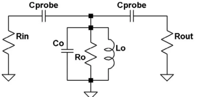
Since the open end of the screw moves with frequency, the probe coupling also varies with frequency. Increased coupling loads the resonator, increasing the bandwidth. The equivalent circuit of a quarter-wave resonator is simply a parallel-tuned circuit, shown in Figure 4. Resonator losses are lumped into an equivalent resistance, Ro, in parallel with the tuned circuit. The resonator has an unloaded Q, QU = Ro/ XLo where XLo is the
Figure 4. Pipe-cap resonator equivalent circuit
In most RF circuits, Rin and Rout are 50 ohms. The coupling capacitors, the probes in this case, transform the effective resistance to a higher value in parallel with Ro, thus reducing the effective resistance across the resonator to a loaded value, RL. This results
in a loaded Q, QL = RL/ XLothat is lower than the unloaded QU. Coupling is proportional to capacitance – a larger capacitor produces more coupling and loads the resonator more. Next, the 3 dB bandwidth (half-power bandwidth) of the loaded resonator may be
calculated11:
L
Q Frequency
BW =
Or we may measure the 3 dB bandwidth BW and then calculate QL. It is difficult to calculate the effective capacitance, inductance, and resistance of a quarter-wave resonator, but measurement of bandwidth is straightforward. From my measurements and those published by WA5VJB, I estimate the unloaded QU of the pipe-cap resonators as 600 to 1000. Pretty good!
Knowing the QU , we can make some estimates of loss. If a resonator is very lightly loaded, for very narrow bandwidth, so that Ro is not much larger than RL, then much of
the power will be dissipated in Ro – resulting in high loss. With more loading, Ro
becomes less significant and more of the power is transmitted. The loss of a resonator may then be calculated12:
dB
20
Loss
Insertion
⎟ ⎟ ⎟ ⎠ ⎞ ⎜ ⎜ ⎜ ⎝ ⎛−
=
L
Q
U
Q
U
Q
log
So for a QU around 1000, the bandwidth can be as narrow as perhaps 1% of the resonant frequency before loss becomes significant, since 1% bandwidth equates to QL = 100, which gives a resonator loss of just under 1 dB. Of course, this loss is in addition to circuit losses – a typical pipe-cap filter loss is 2 or 3 dB total for 1% bandwidth.
Probe Length
The difficulty with pipe-cap filters is finding the right probe length for a desired bandwidth. There is no simple way to estimate the length, and it appears to vary significantly with frequency and to be fairly critical.
I realized this the hard way, while trying to make filters for 2304 and 3456 MHz. I thought that making them a little longer than ones I had used at 5760 MHz would be fine, but the results were not. Tuning was extremely sharp, and the circuit had so much loss that I wondered if the MMIC amplifiers were defective and not amplifying. After spending far too much time troubleshooting, I began to suspect the pipe-cap probes. Since my circuit was not conducive to controlled probe-length experiments, I turned instead to software, simulating the pipe caps using Ansoft HFSS software. Very short probes yielded sharp, lossy response curves, while long ones seemed rather broad. At each resonant frequency, or screw length, the best probe length was proportional to the screw length. Longer screw lengths, for lower frequencies, require much longer probes. I simulated enough data points to make a set of design curves for one-inch pipe caps so that I could predict my filter response. These curves have proven very useful and my circuits now work more predictably.
For future work, both for myself and others, I made similar curves for other common sizes: ¾ - inch, useful at 5760 MHz, and ½ - inch, for 10 GHz.
1” Pipe-Cap Filters
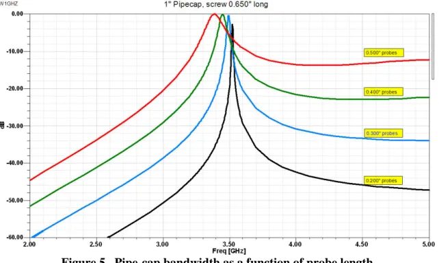
Longer probes increase the coupling to the resonator, lowering the loaded Q, QL , thus increasing the resonator bandwidth, as shown in Figure 5. Some other results are
apparent – not only does the bandwidth increase, but the out-of-band rejection decreases, particularly above the resonant frequency. This may be due to direct coupling between the probes. With shorter probes, the filter gets much sharper, but the loss also increases.
Figure 5. Pipe-cap bandwidth as a function of probe length
The curves in Figure 5 are at one tuning screw setting – the probe length only affects the resonant frequency by a small amount. If the resonant frequency is varied, by tuning the screw, the bandwidth for a given probe length increases with frequency, as shown in Figure 6. However, I have trouble using this curve as a design guide for probe length. If we instead plot bandwidth curves vs probe length for each screw setting, in Figure 7, then it is easier to estimate a good probe length for a desired frequency – just refer back to Figure 3 to estimate the resonant frequency corresponding to each screw length.
1" Pipe-cap Bandwidth
0 25 50 75 100 125 1.5 2.5 3.5 4.5 5.5 6.5 Frequency (GHz) B a nd wi dt h ( M H z ) Probe length 300 mils 400 mil 500 mil 600 mil 700 mil Figure 6Loss is much harder to simulate, since the losses are not in the materials, but in the details. A threaded screw is a rough surface for RF, and rough surfaces increase loss. Even worse is the screw contact to the pipe cap – this is at the maximum current point of the resonator, where even small resistances add loss.
1" Pipe-cap Bandwidth vs Probe Length
0 25 50 75 100 125 200 300 400 500 600 700
Probe Length (mils)
B a n dw idt h ( M H z ) Screw depth 300 mils 600 mils 650 mils 800 mils 850 mils 875 mils Figure 7
So losses are better characterized by measurement. Didier, KO4BB, made a suggestion on the WA1MBA microwave reflector that a pipe-cap filter could be held together by a C-clamp to allow quick adjustments. Since the rim of the pipe cap is in a high-impedance, low current area, contact resistance is not critical. I put together the test fixture shown in Figure 8 and made some measurements using my ancient HP-8410 Network Analyzer. No fancy computer corrections are used, so these numbers aren’t precise.
The measured curves of bandwidth vs probe length for each screw setting, in Figure 9, show bandwidth increasing with probe length for longer probes, but flattening out with shorter probes. What is happening is that the equivalent resistance Ro due to losses is controlling the bandwidth, rather than the loading of the probes. Thus, the bandwidth remains constant but loss increases.
1" Pipe-cap Measured Bandwidth
vs Probe Length
0 25 50 75 100 125 150 200 300 400 500 600Probe Length (mils)
B a ndw idt h ( M H z ) Screw depth 400 mils 500 mils 600 mils 700 mils 775 mils 900 mils Figure 9
The measured losses are plotted in Figure 10. The test fixture seems to add around 1 dB of loss, probably because it is built on ordinary epoxy-fiberglass PC board, rather than good Teflon microwave board. We can see that the loss gets high as we approach the flat area of the curves in Figure 9.
1" Pipe-cap Measured Loss
0 2 4 6 8 10 12 200 300 400 500 600
Probe Length (mils)
Los s ( dB ) Screw depth 400 mils 500 mils 600 mils 700 mils 775 mils 900 mils Figure 10
Plotting the loss vs the relative bandwidth of the resonator is much more illuminating. In Figure 11, we see that the loss increases rapidly for bandwidths less than 1% of the resonant frequency. This fits with our estimate of the unloaded QU around 1000. I also found that taller pipe caps have lower loss, so the QU is apparently higher. The better version, marked “NIBCO”, are about 1.015” high overall, while the shorter ones are about 0.925” high. Obviously, the taller ones will tune to a lower frequency since they can accommodate a longer tuning screw.
1" Pipe-cap Measured Loss
vs Percentage Bandwidth
0 2 4 6 8 10 12 0.0% 1.0% 2.0% 3.0% Bandwidth as Percentage of Resonant Frequency Los s ( dB ) Screw depth 400 mils 500 mils 600 mils 700 mils 775 mils 900 mils Figure 11Since amateur operation is usually within a narrow frequency range, we usually want narrow filters with low loss. With pipe caps, we can make reasonably low loss filters with 3-dB bandwidths in the range of 0.5% to 2% of the resonant frequency – for instance, 17 to 80 MHz bandwidth at 3456 MHz.
While the 3-dB bandwidth is quite narrow, the skirts of a single resonator are not steep, so the out-of-band rejection, 20 or 30 dB down, can be much wider – see Figure 5. If a single resonator does not provide adequate rejection, multiple resonators may be
cascaded. Direct connection will not work predictably, since the resonators will interact and the response will depend on the length of transmission line between them. However, we can isolate the resonators from each other and compensate for the loss at the same time by putting MMIC amplifiers between them. Then each resonator will see a
reasonable termination at each end and behave predictably, and the total response will be the sum of the resonators and amplifiers.
One final note on probe length: all the curves above are for bare probes extending into the pipe cap from a PC board, like the “PCB input” in Figure 1. The results published by
WA5VJB used semi-rigid cable connections, like the “Coax input” in Figure 1, with the center conductor extending into the pipe cap as a probe and the Teflon insulator
extending the whole length of the probe. The Teflon appears to increase the capacitive coupling, so that the response of these probes is similar to a longer bare probe.
1/2” Pipe-Cap Filters
These small pipe caps work well at 10 GHz, and Figure 3 shows that they can be tuned down to about 5 GHz. Curves for the half-inch pipe caps are shown in Figure 12, as a function of resonant frequency, and in Figure 13, as a function of probe length for each tuning screw position. In the latter plot, we can again see the bandwidth leveling off for short probe lengths, an indication of increasing loss. Like the one-inch version, it appears that the loss will increase for 3-dB bandwidths less than 1% of the resonant frequency.
1/2" Pipe-cap Bandwidth
0 50 100 150 200 250 300 350 4 6 8 10 12 Frequency (GHz) B a n d w id th (M H z ) 125 mil probes 150 mil probes 175 mil probes 200 mil probes Figure 121/2" Pipe-cap Bandwidth vs Probe Length
0 50 100 150 200 250 300 350 100 125 150 175 200 225
Probe Length (mils)
B a n d w idth ( M H z ) Screw depth 150 mils 175 mils 200 mils 250 mils 300 mils 400 mils Figure 13
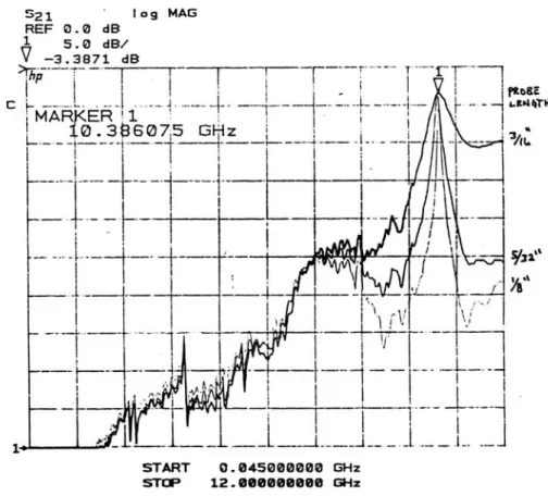
I did not make any measurements for ½ inch pipe-caps, but did scan the measured curves from my 1993 paper3, in Figure 14. At 10.368 GHz, the compromise probe length is about 5/32”; shorter probes are lossy, and longer ones are not sharp enough. The
difference between these three conditions is about 1/32 of an inch, which is about as close as I can control the length. For a 3 dB bandwidth around 1% of 10 GHz, a single
resonator is not selective enough for good LO and image rejection, so multiple pipe-caps were needed. Since each pipe-cap resonator had more than 3 dB of loss at 10 GHz and good MMICs only have around 10 dB of gain, alternating pipe-cap resonators and MMIC amplifiers is a good combination.
3/4” Pipe-Cap Filters
Three-quarter inch pipe caps are ideal for 5760 MHz. I also used them at 3.3 GHz in the multiplier chain of the 10 GHz single-board transverter7. Curves for the ¾ -inch pipe caps are shown in Figure 15, as a function of resonant frequency, and in Figure 16, as a function of probe length for each tuning screw position. In the latter plot, we can again see the bandwidth leveling off for short probe lengths, an indication of increasing loss. Like the one-inch version, it appears that the loss will increase for 3-dB bandwidths less than 1% of the resonant frequency. While I can’t find records from measurements, I recall that the typical loss is lower than the ½ -inch version, probably similar to the one-inch version.
3/4" Pipe-cap Bandwidth
0 50 100 150 200 250 300 2 3 4 5 6 7 8 9 Frequency (GHz) B a n d w id th (MH z ) 200 mil probes 225 mil 250 mil 300 mil 350 mil 400 mil Figure 153/4" Pipe-cap Bandwidth vs Probe Length
0 50 100 150 200 250 300 150 250 350 450
Probe Length (mils)
B a nd w idt h ( M H z ) Screw depth 200 mils 250 mils 300 mils 375 mils 400 mils 500 mils 600 mils 700 mils Figure 16
Larger Pipe-caps
Pipe-caps for larger diameter pipe are not significantly taller than the one-inch variety. Thus, they cannot accommodate much longer screws, so will not operate much lower in frequency. On a printed-circuit board, one would occupy significantly more area, which is hardly an advantage. The only potential advantage might be that the probes could be spaced farther apart, which might improve stopband attenuation.
Summary
Pipe-cap filters are simple and inexpensive microwave filters. The design curves here should help understanding and enable their use in homebrew projects. The curves are useful not just in the ham bands but for other frequencies, such as in multiplier strings or just interesting projects like receiving deep-space probes.
Table 1. Nominal Pipe Cap Dimensions
Size Inner Inside Probe
Diameter Height Spacing
1/2" 0.625" 0.565" 0.375" 3/4" 0.875" 0.880" 0.5"
References
1. Kent Britain, WA5VJB, “Cheap Microwave Filters,” Proceedings of Microwave Update ‘88, ARRL, 1988, pp 159-163. also ARRL UHF/Microwave Project Book, ARRL, 1992, pp. 6-6 to 6-7.
2. Wesolowski, R., DJ6EP, and Dahms, J., DC0DA, “Ein 6-cd-Transvertersystem moderner Konzeption,” cq-DL, January 1988, pp. 16-18.
3. Wade, P., N1BWT, “Building Blocks for a 10 GHz Transverter,” Proceedings of the 19th Eastern VHF/UHF Conference, ARRL, 1993, pp. 75-85.
4. Wade, P., N1BWT, “Mixers, etc. for 5760 MHz,” Proceedings of Microwave Update ’92, ARRL, 1992, pp. 71-79.
5. Wade, P. N1BWT, “A Dual Mixer for 5760 MHz with Filter and Amplifier,” QEX, August 1995, pp. 9-13. also www.w1ghz.org/10g/QEX_articles.htm
6. Wade, P., N1BWT, “A Single-Board Transverter for 5760 MHz and Phase3D,” QEX, November 1997, pp. 2-14. also www.w1ghz.org/10g/QEX_articles.htm
7. Paul Wade, W1GHZ, “A Single-Board Transverter for 10 GHz,” Proceedings of the 25th Eastern VHF/UHF Conference, ARRL, 1999, pp. 75-85. also in
Andy Barter, G8ATD, ed., International Microwave Handbook, RSGB & ARRL, 2002, pp. 365-372.
8. www.downeastmicrowave.com 9. www.db6nt.com
10.www.ansoft.com
11.Karl F. Warnick & Peter Russer, Problem Solving in Electromagnetics, Microwave Circuit, and Antenna Design for Communications Engineering, Artech, 2006, p. 192. 12.Harlan H. Howe, Stripline Circuit Design, Artech, 1974, p. 215.