Received March 2nd, 2016, 1st Revision October 18th, 2016, 2nd Revision February 6th, 2017, Accepted for
Production and Delivery Batch Scheduling with Multiple
Due Dates to Minimize Total Cost
Endang Prasetyaningsih*, Suprayogi, T.M.A. Ari Samadhi & Abdul Hakim Halim Department of Industrial Engineering and Management,
Faculty of Industrial Technology, Institut Teknologi Bandung, Jalan Ganesha 10, Bandung 40132, Indonesia
*
E-mail: [email protected]
Abstract. This paper addresses an integrated production and delivery batch scheduling problem for a make-to-order environment over daily time period, where the holding costs of in-process and completed parts at a supplier location and of completed parts at a manufacturer location are distinguished. All orders of parts with different due dates from the manufacturer arrive at the same time. The parts are produced in production batches and subsequently the completed parts are delivered in delivery batches using a capacitated vehicle in order to be received at the respective due dates. This study was aimed at finding an integrated schedule of production and delivery batches so as to meet the due date at minimum total cost consisting of the corresponding holding cost and delivery cost. The holding cost is a derivation of the so-called actual flow time (AFT), while the delivery cost is assumed to be proportional to the number of deliveries. The problems can be formulated as an integer non-linear programming model, and the global optimal solution can be obtained using optimization software. A heuristic algorithm is proposed to cope with the computational time problem using software. The numerical experiences show that the proposed algorithm yields near global optimal solutions.
Keywords: actual flow time; backward scheduling; batch scheduling; integer non-linear programming; integrated production and delivery.
1
Introduction
To deal with customer satisfaction measured by on-time delivery, most companies keep a decent number of inventory items. However, fierce competition in today’s global market forces many companies to increase their operational performance by reducing inventory levels and offering a faster response to the market. Reducing inventory levels leads to a closer linkage between production and delivery functions, so that it is necessary to make an integrated schedule of both operations. Integrated scheduling – the so-called integrated production and outbond delivery scheduling (IPODS) – is often used to generate a detailed activity schedule for production and delivery over short periods of time, which is then implemented in daily operations. As a
consequence, the finished products are often delivered to customers immediately or soon after production [1].
IPODS problems represent a combination of modeling parameters of both the production and the delivery stage with a single variable to be optimized or a list of variables in case of a multi-criteria optimization of time-based, cost-based, and revenue-based performance measures [1,2]. Various IPODS models can be seen in a make-to-order environment with a short lead-time [3,4], or in time-sensitive products [5,6]. The IPODS model consists of job scheduling at the production stage and of batch scheduling at the delivery stage [7,8], or batch scheduling in both the production and the delivery stage [9,10]. Most IPODS models adopt a forward scheduling approach, which cannot guarantee to meet the due date. Table 1 shows the detailed parameters used by [3-10].
This study was motivated by the practical situation of a production and delivery scheduling problem for a make-to-order environment involving a single car-seat supplier and a single car manufacturer. The manufacturer adopts a pull-system approach in which production is based on the actual daily demand, so that the production rate at the supplier is determined by the daily orders from the manufacturer. The orders for car seats with different due dates arrive from the manufacturer at the same time. The car seat parts arrive in production batches at the beginning of the processing time and the car seats are then delivered in delivery batches to the manufacturer assembly line on the same day. Hence, in order to meet the due date, the car seats should be delivered immediately after they have been assembled [11]. This situation forces the supplier to integrate both the production and the delivery stage. Because the delivery vehicle’s capacities are limited, the batches have to be delivered in several runs. This increases the number of deliveries but decreases the waiting time of the batches. Thus, the problem is how to determine the number of delivery batches that results in the minimum of waiting time.
The car-seat problem is an IPODS problem that schedules production and delivery batches simultaneously. This problem has been studied in [12] and [13], which considered a single machine to process the parts, and the completed parts were delivered using sufficient multiple vehicles in order to be received at a common due date, where the holding costs of in-process and completed parts at the supplier location and of completed parts at the manufacturer location were distinguished. AFT performance was used, adopting a backward scheduling approach in order to minimize the time of the parts flowing in both stages and meet the due date simultaneously. AFT performance has been applied in [14-16] and [17] in various batch scheduling problems at the production stage. A brief description of AFT will be given in Section 3.
This study was aimed at developing the work of [12] and [13] by extending a common due-date case to become a multiple due-date case. It was assumed that the supplier has one vehicle. Future research will be aimed at solving the problem for multiple vehicles.
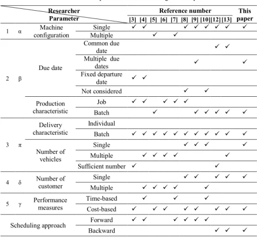
To describe this research’s position, the IPODS models classified in [1] are used where the scheduling problems are represented according to five parameters, i.e. α|β|π|δ|γ, which specify the machine configuration in the production plants, the order restrictions and constraints, the characteristics of the delivery process, the number of customers, and the objective function, respectively [1]. The characteristic of this research is that the order has multiple due dates processed on a single machine in production batches. The order is delivered to one customer using one vehicle in delivery batches. This research adopted a backward scheduling approach to minimize total cost. Table 1 shows this research’s position among some IPODS problems.
Table 1 Position of present research among IPODS problems.
Researcher Parameter
Reference number This paper [3] [4] [5] [6] [7] [8] [9] [10][12] [13] 1 α Machine configuration Single Multiple 2 β Due date Common due date Multiple due dates Fixed departure date Not considered Production characteristic Job Batch 3 π Delivery characteristic Individual Batch Number of vehicles Single Multiple Sufficient number 4 δ Number of customer Single Multiple 5 γ Performance measures Time-based Cost-based
Scheduling approach Forward
The rest of this paper is organized as follows. Section 2 describes the problem definition. In Section 3 we briefly describe the AFT. Section 4 explains the model formulation. Section 5 describes the solution method. Section 6 explains the heuristic solution and the numerical experiences. Section 7 contains comparison tests. Section 8 contains a discussion of the results. Section 9 contains concluding remarks and further research suggestions.
2
Problem Definition
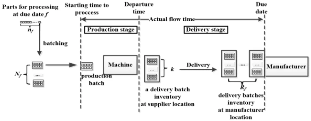
The problem to be discussed is illustrated in Figure 1 and can be described in detail as follows. Let us assume that a supplier receives an order for a single item with multiple due dates. There are parts requested at u different due dates 1, … , sorted from the longest due date. A number of parts is first grouped into containers with capacity c and is considered a production batch. The completed batches are then delivered times using a single vehicle that can carry up to k production batches. The production batches,
1, … , ; 1, … , ; 1, … , , with batch sizes are processed on a
single machine at the production stage within a given and fixed processing time, t, for each part. Each production batch requires a setup activity within s, which is assumed to be constant. It is also assumed that the setup activity does not require any materials, so that the production batches can arrive at the production stage at their starting time of processing, . Each part in a production batch must wait in the batch until all the parts are completed at , which incurs a holding cost for in-process parts.
Figure 1 Scheme of the discussed problem.
Each completed batch must wait until k production batches are completed and then they are delivered in one shipment using a single capacitated vehicle. This is considered a delivery batch and incurs a holding cost at the supplier location.
The vehicle departs from the supplier location at within transportation time v and should arrive at the manufacturer location at 1, … , ;
1, … , . However, the delivery batches should be received by the
manufacturer at the respective due date, so that completed batches that arrive before the respective due date must be held during − in a supplier’s warehouse located at the manufacture’s. This incurs a holding cost for completed parts at the manufacturer location.
The two problems are how to batch the parts requested for the respective due date 1, … and how to schedule the resulting batches during the production and the delivery stages so as to meet the due date at minimum total cost which consists of the holding cost for both stages and the delivery cost. The planning horizon is the time from time zero to the longest due date. The problem discussed is called a single-machine one-vehicle multi-due date (SMOVMD) problem.
The following notations will be used throughout this paper.
Indexes
=
Index identifying the position, counted from the due date position on a time scale, of a batch on an integrated production and delivery schedule=
Index identifying the delivery batch number=
Index identifying the due date numberSets
=
Symbol for delivery batch number 1, … , at due date 1, … ,=
Symbol for production batch, sequenced in position1, … , of delivery batch number 1, … , at due date
1, … ,
Parameters
c = Container capacity
!, " = Procurement cost of container and the transportation cost of each delivery during the scheduling period, respectively #, $ = Holding cost per unit time for a completed part at the supplier
location and at the manufacturer location, respectively % = Holding cost per unit time for an in-process part
= Due date number f k = Vehicle capacity
= Demand rate at due date f s = Setup time of a batch
t = Processing time of a part
& = Production time of k production batches
&' = Processing time of batch
v = Transportation time from supplier to manufacturer or vice versa
Decision Variables
= Departure time of the vehicle loaded by batch
, = Starting time of processing batch and batch , respectively
, = Arrival time of delivering batch and completion time of processing batch , respectively
(), (), () = AFT of total parts in batch , in batch , and in all batches during both production and delivery stages, respectively
*# , *$ = Holding time of completed parts in batch at the supplier and at manufacturer locations, respectively
*% = Holding time of in-process parts in batch ,
+ = Number of batch
+ = Number of production batches at due date f
+! = Number of containers = Size of batch
= Size of batch
= Number of deliveries on due date 1, … ,
, = Binary variable of the procurement cost of a container, which is 1 if batch needs a container, and 0 otherwise
- = Idle time of the production facility on due date f for delivery number
- ./ = Idle time due to the vehicle limitation between due dates
− 1 and
3
Actual Flow Time of Production and Delivery Batch
Scheduling
AFT performance applied at the production stage regardless of transportation time has been proposed in [14]. The AFT of a batch, ( , is defined by [14] as the time the batch spends in the shop from the starting time of its processing,
( − , 1, … , + (1) In a batch scheduling problems, parts in a batch must wait in the batch until all parts from the batch are completed. Therefore, the AFT of each part in a batch is the same as the AFT of the batch. Thus, the AFT of total parts in batch can be calculated by multiplying the AFT of the batch by the number of parts in the batch, [14]. Hence, the AFT, (), of the parts in batch is formulated as follows:
() − , 1, … , + (2)
The AFT performance has been developed in [12] for both the production and the delivery stage and is defined as the interval of time between the arrival time of a batch at the production stage and its due date, i.e. the time at which the batch is received by the manufacturer.
We adopt a backward scheduling approach, so that the last delivery batch should be scheduled first by arranging the arrival time of the batch at the manufacturer location closest to its due date, and the completion time of the last production batch of that delivery coincides with its departure time. Meanwhile, the first production batch of that delivery, i.e. production batch number k, should be scheduled later. Hence, the AFT of a delivery batch at due date f can be defined as the interval between the arrival time, 0 , of production batch 0, and its due date, . Referring to Eq. (2), the AFT, () , of the parts in delivery batch can be formulated as follows in Eq.(3):
() 1 −
0 2 , 1, … , ; 1, … , (3)
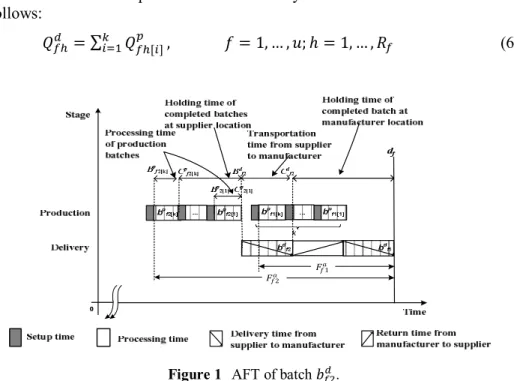
Accordingly, the AFT of all parts in a batch involves the holding time of the completed parts in the batch at the manufacturer location and at the supplier location, the transportation time, and the holding time of in-process parts in a batch (see Figure 2). Hence, the AFT of the parts in a delivery batch, (), can be expressed with the following equation:
() 3 − − − − ∑ 510 − 2 −
6/
1 − 278 , (4)
1, … , ; 1, … ,
The fourth term of the right-hand side of Eq. (4) states the processing time of a batch, which can be rewritten as follows:
1, … , ; 1, … , ; i 1, … ,
The relation between production and delivery batch sizes can be rewritten as follows:
∑0
6/ , 1, … , ; 1, … , (6)
(:1
(:2
Figure 1 AFT of batch <.
The AFT of all parts during the production and the delivery stage, (), can be developed by applying Eqs. (5) and (6) to Eq. (4), and is formulated as follows:
() ∑ ∑=> − 6/ ? 6/ + ∑?6/∑=>6/ − + ∑ ∑ ∑0 6/ 1 − 2 => 6/ ? 6/ + ∑ ∑ ∑ & 1 2 < 0 6/ => 6/ ? 6/ (7)
4
Model Formulation
The following assumptions are applied in formulating the SMOVMD model: 1. The total number of processed parts is equal to the total demand
2. The transportation time includes packing, loading and unloading the batches 3. The production batch size cannot excess the container’s capacity
4. The vehicle capacity is stated as the number of production batches instead of the number of parts
5. The distance between the supplier’s warehouse and the reception location of the completed parts is neglected
6. The opportunity cost of either the vehicle or the container being idle is omitted
7. The delivery cost is proportional to the required number of deliveries regardless of the batch size
8. The holding cost increases due to the added value of parts from the production line to the manufacturer location
The objective of the SMOVMD problem is to minimize the total cost (TC), which consist of holding cost and delivery cost. The holding cost constitutes a derivation of the AFT, whereas the delivery cost is assumed to be proportional to the number of deliveries. In addition, there is a cost that does not constitute a derivation of the AFT but must also be taken into account, i.e. the procurement cost of container !. The total cost of the SMOVMD problem is then formulated as follows:
A $*# + " + #*$ + %*% + !+! (8)
Applying Eq. (7) to Eq. (8) yields the objective function of the SMOVMD problem as follows in Eq. (9):
Minimizing A $∑ ∑=> − 6/ ? 6/ + "∑?6/ + #∑ ∑ ∑0 6/ 1 − 2 => 6/ ? 6/ + %∑ ∑ ∑ & 10 2< 6/ => 6/ ? 6/ + !, (9) Subject to: , & &' , ∀ ; ∀ ; ∀ (10) ∑0 , 6/ , ∀ ; ∀ (11) , ≤ , ∀ ; ∀ ; ∀ (12) ∑= 6/ , ∀ (13) //+ D /, (14) /+ D ≤ , 2, … , ; 1 (15) ./ − 2D − 0, ∀ ; 2, … , (16) + D − 0, ∀ ; ∀ (17) < ./, ∀ ; 2, … , (18) < ./ ,=>GH, 2, … , ; ∀ (19)
/ / + &'/ / − / 0, ∀ (20) − ./ + I, ./ + &' 0, ∀ ; ∀ ; 2, … , (21) ./ 0 − I, ./ / − - − &' / − / 0 (22) ∀ ; 2, … , ./ =>GH0− I, ./ =>GH 0 − - ./ − &'/ / − / / 0, (23) 2, … , + &' − 0, ∀ ; ∀ ; ∀ (24) ./ 0 − I, ./ 0 − - − ≤ 0, ∀ ; 2, … , (25) ./ =>GH 0 − I, ./ =>GH 0 − - ./ − /≤ 0, (26) 2, … , / / − ./ / ≤ 0, 2, … , (27) , ∈ K0,1L , ∀ ; ∀ ; ∀ (28) , ≥ 0 and integer, ∀ ; ∀ ; ∀ (29) , , , , - , - ./ ≥ 0, ∀ ; ∀ ; ∀ (30)
Eq. (10) implies the processing time of each production batch. Eqs. (11) and (12) show the restriction of the batch sizes. Eq. (13) states a material balance in both stages. Eq. (14) ensures that the first delivery batch at the first due date in the schedule arrives at the manufacturer location coinciding with its due date. Eq. (15) shows that the first delivery batch at the second due date and at the subsequent one in the schedule may not arrive at the manufacturer location on the respective due date. Eqs. (16) and (17) represent the departure time and the arrival time of the vehicle at the manufacturer location, respectively. Eqs. (18) and (19) ensure that transportation activities will not overlap. Eqs. (20) to (23) represent the starting time of processing the batches, while Eq. (24) represents the completion time of processing the batches. Eqs. (25) and (26) represent the idle times. Eq. (27) ensures that the vehicle will depart after the production batches are completed. Eq. (28) shows the binary variable, Eq. (29) shows that the batch sizes must be integer and non-negative, while Eq. (30) represents the non-negative constraint.
5
Solution Method
The number of deliveries variable, , can be relaxed by calculating
⁄ , where does not have to be an integer. This means that the deliveries do not have to be composed of exactly equal shipment sizes, a so-called imperfect matching situation [18]. If the deliveries consist of exactly equal shipment sizes, then such a situation is called a perfect matching situation. Referring to [18], a perfect matching situation occurs if is an integer and an imperfect matching situation occurs if is not an integer. However, intuitively, the number of deliveries should be an integer, so is rounded up. Relaxation of allows both problems of the SMOVMD model to be solved simultaneously using optimization software. Example 1 shows how the SMOVMD model is solved.
Example 1.
Consider a case where / 100; < 50; / 200; < 130; D 20;
3; 20; & 0.5; I 2; ! 25; " 50; # 20; % 0.75 #;
$ 1.5 #. This means that 100 demanded parts / must be received by the manufacturer at / 200, and 50 demanded parts < must be recieved at
< 130.
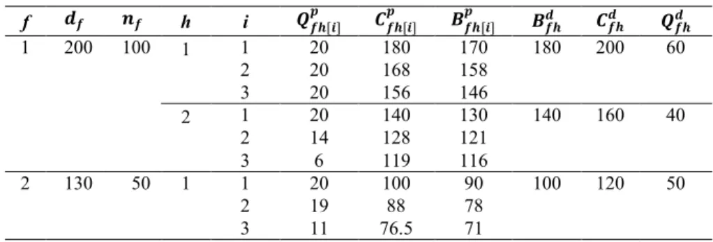
The SMOVMD problem was solved using Lingo 11.0 software running on a PC with an Intel Core i3-3240 CPU @ 3.40GHz with 4 GB of RAM. In this example, Lingo reports a global optimal with a TC of 113,740. Table 2 shows the resulting batch sizes and their schedule, while Figure 2 shows the Gantt chart. Table 2 shows that there are 6 production batches with 2 deliveries at
/ 200, and 3 production batches with 1 deliveries at < 130. Table 2 Computational result of example 1.
f YZ [Z h i \Z] ^_ `_Z] ^ aZ] ^_ aZ]Y `Z]Y \Z]Y 1 200 100 1 1 20 180 170 180 200 60 2 20 168 158 3 20 156 146 2 1 20 140 130 140 160 40 2 14 128 121 3 6 119 116 2 130 50 1 1 20 100 90 100 120 50 2 19 88 78 3 11 76.5 71
d1=200 d2=130 4 Q p 111 =20 Qp 112 =20 Qp 113 =20 Qp 121 =20 Qp 122 =14 bd 11;Qd11= 60 170 158 146 180 168 156 130 121 140 128 116 180 144 Qp 123 =6 119 114 Qp 211 =20 Qp 212 =19 90 78 88 71 Qp 213 =11 76,5 100 bd 12;Q d 12= 40 bd 21;Qd21= 50 14 Idle 140 100 10 120 160 Idle Production Delivery Time Stage
Figure 2 Gantt chart of Example 1.
Figure 2 shows that delivery batch // departs at 180 and it arrives at the manufacturer location on its due date, / 200. Meanwhile, delivery batch </ must depart at t = 100 and arrives at t = 120, although due date < 130. Delivery batch </ cannot depart at t = 110 because the delivery must be finished at t = 140. To show the characteristics of the SMOVMD model, we conducted several various problem sizes of the perfect and imperfect matching situations. We considered the transportation time from the supplier to the manufacturer and vice versa, 2v, being longer or shorter than the production time of k production batches, & . Table 3 shows the CPU time to solve the SMOVCD problem with v = 10 and v = 20, where v = 10 represents 2D < & , and v = 20 represents 2D > & .
Table 3 CPU time for various sizes.
Case Z YZ [Z v = 10 v = 20
TC CPU time TC CPU time
Perfect matching 1 1 200 120 211,700 00:00:00 274,100 00:00:00 2 130 120 2 1 400 120 440,675 (local optimal) interrupted after 5 hours 524,675 00:26:59 2 300 120 3 200 180 3 1 500 120 710,370 (local optimal) interrupted after 5 hours 1,057,725 (local optimal) interrupted after 5 hours 2 450 180 3 400 60 4 150 180 Imperfect matching 4 1 200 100 87,540 04:02:00 113,740 01:06:00 2 130 50 5 1 300 40 98,285 (local optimal) interrupted after 5 hours 124,485 05:02:05 2 200 100 3 130 50 6 1 400 120 200,535 (local optimal) interrupted after 5 hours 243,535 (local optimal) interrupted after 5 hours 2 300 40 3 200 100 4 130 50
From Table 3, we find that for the problem with 4 due dates in the perfect and imperfect matching cases when the demand rates are different, a global optimal solution cannot be found, even though the computations were run for 5 hours. However, at the same demand rate for perfect matching cases, the computations were very fast (see Case 1). This finding indicates that if the numbers of the due dates are increased or the demand rates are different, the computational time increases sharply. Hence, it is important to develop a heuristic solution to cope with the computational time problem.
6
Heuristic Solution
The problem of batch scheduling that minimizes () can be stated as searching for batch sizes and batch schedules. Once the batch sizes are determined, the remaining problem is to schedule the resulting batches [14]. For the production stage, the optimal backward schedule that minimizes () is obtained from arranging the batches in order of non-increasing batch sizes [14]. Meanwhile, in the IPODS model, for the problem of a single machine with %< # that minimizes total cost, there exists an optimal forward schedule wherein the jobs in each delivery batch are scheduled according to their production in LPT order [8]. According to [14] and [8], the following procedure can be used to sequence and schedule the production and delivery batches.
Theorem 1. Suppose that there is a scheduling period with u due dates
1, … , . There are parts requested at the respective due date. The parts are
grouped to become + production batches and are processed on a single machine with the same setup time and processing time. The + completed batches are then delivered in R times using a single capacitated vehicle, which can carry up to k production batches, which is considered one delivery batch. The backward schedule that minimizes total actual flow time is obtained from arranging the delivery batches according to their production in order of non-increasing batch sizes:
/ / ≥ ⋯ ≥ / 0 ≥ ⋯ ≥ < / ≥ ⋯ ≥ < 0 ≥ ⋯ ≥ = / ≥ ⋯ ≥ = 0
Proof. This theorem can be proven using a pairwise interchange rule.
According to [14], we propose a heuristic algorithm to solve the SMOVMD model by breaking the problem into two sub-problems, i.e. batching and scheduling as follows:
1. Batching
This sub-problem is aimed at determining the number and sizes of both the production and the delivery batch. The number of production batches of each due date variable, + , can be relaxed by dividing parts by container capacity
c, ⁄ . We then set + − 1 batches is equal to c, and 1 batch is equal to the remaining parts, i.e. d − + − 1 e.
The + production batches are then arranged using Theorem 1, i.e. the batches are sequenced in non-increasing batch sizes from the due date position. The number of deliveries, , is determined by grouping the consecutive k production batches as one delivery batch. Intuitively, , is an integer, so that it is rounded up, i.e., f+ ⁄ g. The size of each delivery batch is obtained by adding up the parts in the k consecutive production batches.
2. Scheduling
This sub-problem is aimed at scheduling the resulting batches of the batching sub-problem by adopting a backward scheduling approach to guarantee that the first delivery batch expected at the first due date in the schedule arrives at the manufacturer location at its due date, // /. However, the first delivery batch at the second due date and at the subsequent one in the schedule cannot be guaranteed to arrive at the manufacturer location at its due date because of the vehicle’s capacity limitation.
The arrival time of each vehicle at the second due date and at the subsequent one in the schedule, , is obtained by comparing its due date, , and the time the vehicle is available, i.e. 1 ./ =>GH − D2. There are two possible relations and their decisions: if ≤ 1 ./ =>GH − D2, then set ; otherwise, set
1 ./ =>GH − D2. The departure time of the vehicle is then determined by calculating − D.
Once the departure time of a delivery batch is determined, the starting time of processing the production batch at the first position in the schedule can be obtained. This shows that the production and delivery batches should be scheduled simultaneously in order to find a feasible schedule.
6.1
Algorithm
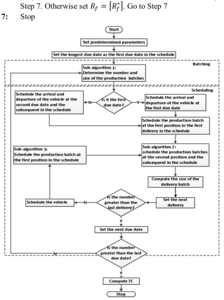
Considering both problems, we propose the SMOVMD algorithm and sub-algorithms 1, 2 and 3 to solve the SMOVMD problem represented in Figure 3. The algorithm can be described in detail as follows:
SMOVMD Algorithm
Step 1: Set predetermined value of parameters , , D, , , I, &, , %, #, $, !, and ". Go to Step 2.
Step 3: Using Sub-algorithm 1, determine the number and size of the production batches. Go to Step 4.
Step 4: If 1, then go to Step 5. Otherwise go to Step 13.
Step 5: For 1, set and − D. Go to Step 6.
Step 6: For 1, set )for : ; , 1; ; and
− & . Go to Step 7.
Step 7: Using Sub-algorithm 2, schedule the second production batch and the subsequent one in the schedule. Go to Step 8.
Step 8: Set the k consecutive production batches as a delivery batch, and compute ∑06/ . Go to Step 9.
Step 9: Set + 1. If ≤ , then go to Step 10. Otherwise, go to Step 15.
Step 10: Set ./ − D; − D. Go to Step 11.
Step 11: Schedule the first production batch in the schedule using Sub-algorithm 3. Go to Step 12.
Step 12: Schedule the second production batch and the subsequent one in the schedule using Sub- algorithm 2. Back to Step 9.
Step 13: Set 1. Determine the arrival time of the vehicle at the manufacturer location, , by comparing due date and the time the vehicle is available, 1 ./ =>GH − D2. If ≤ 1 ./ =>GH −
D2 then set . Go to Step 14. Otherwise, set
1 ./ =>GH − D2. Go to Step 14.
Step 14: Set − D. Back to Step 6.
Step 15: Set + 1; go to Step 16.
Step 16: If > then compute TC using Equation (9). Go to Step 17. Otherwise, back to Step 3
Step 17: Stop
Sub-algorithm 1 (Batching)
Step 1: Compute +∗ ⁄ . Go to Step 2
Step 2: Compute + f+∗g, and go to Step 3
Step 3: Set the batch size ) for : 1, … , + − 1 , and ) −
+ − 1 for : + . Go to Step 4.
Step 4: Arrange the production batches with size ) for : 1, … , + starting from : 1 to : + from the due date position (where the first production batch is put at − D , and add setup time s before processing each batch. Go to Step 5
Step 5: Compute ∗ ⁄ . Go to Step 6
Step 6: If ∗ is an integer, then set the number of deliveries, ∗. Go to Step 7. Otherwise set f ∗g. Go to Step 7
Step 7: Stop
Figure 3 The SMOVMD algorithm.
Sub-algorithm 2 (scheduling the production batch at the second due date and at the subsequent one in the schedule)
Step 1: Set 2. Go to Step 2
Step 2: If > then go to Step 6. Otherwise, set the sizes of production batch, ) for : + − 1 . Go to Step 3
Step 3: If 0, then set , 0. Otherwise, set , 1.
Step 4: Go to Step 4
Step 5: Compute the completion time ./ − I, ./ and
calculate the starting time − & . Go to Step 5
Step 6: Set + 1. Back to Step 2
Step 7: Stop
Sub-algorithm 3 (Scheduling the first production batch in the schedule)
Step 1: For 1, set production batch sizes ) for : +
− 1 and set , 1. Go to Step 2
Step 2: Determine the completion time of production batch by comparing the departure time and 1 ./ 0 − I2.
Step 3: If < 1 ./ 0 − I2, then set . Go to Step 3
Step 4: Otherwise, set 1 ./ 0 − I2. Go to Step 3
Step 5: Set − & . Go to Step 4
Step 6: Stop
6.2
Numerical Experience
Example 2 is presented here to show how the SMOVMD algorithm can solve the problem.
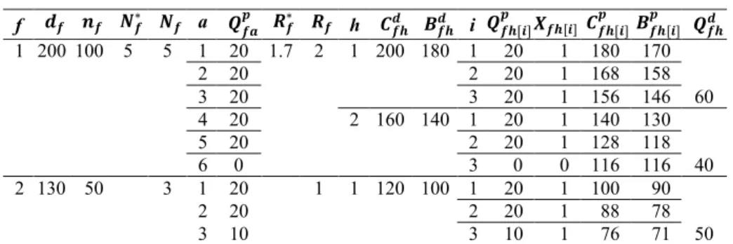
Example 2. Consider Example 1 and solve the model using the SMOVMD algorithm. Table 4 shows the computational result of Example 2.
Table 4 Computational result of example 2.
f YZ [Z iZ∗ iZ a \Zj_ kZ∗ kZ h `Z]Y aZ]Y i \Z] ^_ lZ] ^ `Z] ^_ aZ] ^_ \Z]Y 1 200 100 5 5 1 20 1.7 2 1 200 180 1 20 1 180 170 60 2 20 2 20 1 168 158 3 20 3 20 1 156 146 4 20 2 160 140 1 20 1 140 130 40 5 20 2 20 1 128 118 6 0 3 0 0 116 116 2 130 50 3 1 20 1 1 120 100 1 20 1 100 90 50 2 20 2 20 1 88 78 3 10 3 10 1 76 71
Example 2 shows that the SMOVMD algorithm solves the SMOVMD problem with resulting a TC of 113,900. From Table 4, we can see that there are 5 production batches for /, which differs from the solution obtained using Lingo software. From this example, we find that the difference in the objective between using Lingo and the SMOVMD algorithm is 0.14%.
7
Comparison Tests
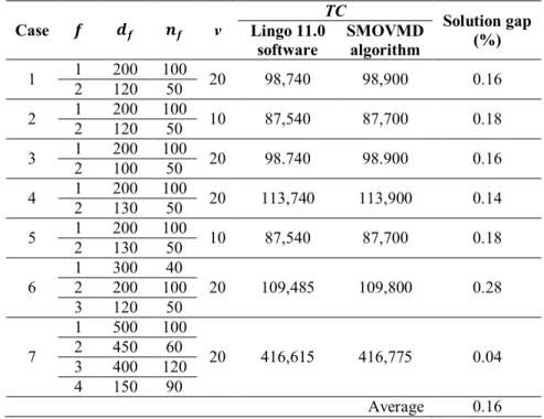
The SMOVMD algorithm is solved manually, so that the computational time cannot be measured. Hence, performance of the SMOVMD algorithm is obtained by calculating the average solution gap of the cost obtained from the SMOVMD algorithm and the optimal solution obtained from the software. The solutions of the perfect matching situation have a similar pattern, whether obtained from Lingo or the SMOVMD algorithm. Hence, to test the performance of the SMOVMD algorithm, we randomly generated more than 25 imperfect matching cases, where the transportation time was predetermined as 10 or 20; the demand rates were taken from interval (10,120), the numbers of due dates were taken from interval [2,4] with the respective due dates taken frominterval (100,500). The comparison tests of 7 cases, represented by 2, 3, and 4 due date cases, are displayed in Table 5. The solution gaps (%) shown in the table were obtained by [{(SMOVMD algorithm solution – Lingo solution)/Lingo solution} × 100].
Table 5 Results of comparison tests ( 3; 20; & 0.5; I 2; ! 25; " 50; # 20; % 0.75 I). Case Z YZ [Z v TC Solution gap (%) Lingo 11.0 software SMOVMD algorithm 1 1 200 100 20 98,740 98,900 0.16 2 120 50 2 1 200 100 10 87,540 87,700 0.18 2 120 50 3 1 200 100 20 98.740 98.900 0.16 2 100 50 4 1 200 100 20 113,740 113,900 0.14 2 130 50 5 1 200 100 10 87,540 87,700 0.18 2 130 50 6 1 300 40 20 109,485 109,800 0.28 2 200 100 3 120 50 7 1 500 100 20 416,615 416,775 0.04 2 450 60 3 400 120 4 150 90 Average 0.16
It can be seen from Table 5 that the average solution gap between Lingo software and the SMOVMD algorithm was 0.16%, which is negligible.
8
Discussion
In Table 5, we consider the transportation time from the supplier to the manufacturer and vice versa, 2v, as longer or shorter than the production time of k production batches, & . If 2D > & , as can be seen in Examples 1 and 2, then it incurs an idle time, i.e. the time the production facilities have to wait to produce the next production batch in the schedule. From Table 3, we can observe that the idle time at the second delivery and the first due date in the schedule, -/<, occurs because the vehicle is available at t = 140. Hence, production batches
/</, … , /<m have to be completed at t = 140 instead of t = 144 in order to find a feasible schedule. From this case we can see that to find a feasible schedule, the production schedule must consider the delivery schedule, and hence that the production and delivery stages must be scheduled simultaneously.
From Table 5, it can be seen that the SMOVMD algorithm is not guaranteed to find a global optimal solution but yields a near global optimal solution. Thus, the SMOVMD algorithm is effective in solving the SMOVMD problem and the steps are traceable and visible.
9
Concluding Remarks
This paper addressed a model of the integrated production and delivery batch scheduling problem considering one vehicle and multiple due dates (SMOVMD) with AFT performance adopting a backward scheduling approach to meet the due date at minimum total cost. The model was formulated as an integer non-linear programming model and solved simultaneously to find a global optimal solution. A new heuristic SMOVMD algorithm, which divides the problem into two sub-problems, i.e. batching and scheduling, was proposed to cope with the computational time problem using software. Based on the numerical experiences, the SMOVMD algorithm yields a near global optimal solution.
In future research a model will be developed that considers multiple vehicles to deliver the completed batches in order to reduce the idle time problem.
References
[1] Chen, Z-L., Integrated Production and Outbound Distribution Scheduling: Review and Extension, Operations Research, 58(1), pp. 130-148, 2010.
[2] Meinecke, C. & Scholz-Reiter, B., A Representation Scheme for Integrated Production and Outbound Distribution Models, Int. J. Logistics System and Management, 18(3), pp. 283-301, 2014.
[3] Zhong, W., Chen, Z.L. & Chen, M., Integrated Production and Distribution Scheduling with Committed Delivery Dates, Operations Research Letters, 38, pp. 133-138, 2010.
[4] Li, S. & Li, M., Integrated Production and Distribution Scheduling Problems Related with Fixed Delivery Departure Dates and Number of Late Orders, Journal of Inequalities and Applications, 2014(409), 2014. [5] Farahani, P., Grunow, M. & Gunther H.O., Integrated Production and
Distribution Planning for Perishable Food Products, Flex. Serv. Manuf.,
24, pp. 28-54. 2012.
[6] Sayedhoseini, S.M. & Ghoreysi, S.M., An Integrated Model for Production and Distribution Planning of Perishable Products with Inventory and Routing Consideration, Mathematical Problems in Engineering, Article ID 475606, 10 pages, 2014 http://dx.doi.org/10.1155/2014/475606 (4 December 2015).
[7] Wan, L. & Zhang, A., Coordinated Scheduling on Parallel Machines with Batch Delivery, Int. J. Production Economics, 150, pp. 199-203, 2014.
[8] Lee, I.S. & Yoon, S.H., Coordinated Scheduling of Production and Delivery Stages with Stage-Dependent Inventory Holding Costs, Omega,
38, pp. 509–521. 2010.
[9] Wang, D., Grunder, O. & El Moudni, A., Single Item Production-Delivery Scheduling Problem with Stage-Dependent Inventory Cost and Due Date Considerations, International Journal of Production Research,
51(3), pp. 828-846, 2013.
[10] Gao, S., Qi, L. & Lei, L., Integrated Batch Production and Distribution Scheduling with Limited Vehicle Capacity, Int. J. Production Economics,
160, pp. 13-25, 2015.
[11] Iyer, A.V., Seshadri, S. & Vasher, R., Toyota Supply Chain Management, a Strategic Approach to the Principles of Toyota’s Renowned System, McGraw Hill, New York, United States, 2009.
[12] Prasetyaningsih, E., Suprayogi, Samadhi, T.M.A.A. & Halim, A.H., Model of Integrated Production and Delivery Batch Scheduling under JIT Environment to Minimize Inventory Cost, Proceedings of the 2014 International Conference on Industrial Engineering and Operations Management, Bali, Indonesia, pp. 2109-2117, 2014.
[13] Prasetyaningsih, E., Suprayogi, Samadhi, T.M.A.A. & Halim, A.H., Production and Delivery Batch Scheduling with a Common Due Date and Multiple Vehicles to Minimize Total Cost, IOP Conference Series: Materials Science and Engineering, 114(1), 012079, 2016.
[14] Halim, A.H., Miyazaki, S. & Ohta, H., Batch-Scheduling Problems to Minimize Actual Flow Times of Parts Through the Shop under JIT Environment, European Journal of Operational Research, 72, pp. 529-544, 1994.
[15] Halim, A.H. & Ohta, H., Batch-Scheduling Problems to Minimize Inventory Cost in the Shop with Both Receiving and Delivery Just In Time, Int. J. Production Economics, 33, pp. 185-194, 1994.
[16] Zahedi, Samadhi, T.M.A.A., Suprayogi & Halim, A.H., Integrating Batch Production and Maintenance Scheduling on a Deteriorating Machine to Minimize Production and Maintenance Costs in Just In Time Environment, Proceedings of APIEMS Conference, Jeju, South Korea, pp. 2061-2069, 2014.
[17] Hidayat, N.P.A., Cakravastia, A., Samadhi, T.M.A.A. & Halim, A.H., A Batch Scheduling for m Heterogeneous Batch Processor, International Journal of Production Research, 54(4), pp.1-16, 2015.
[18] Golhar, D.Y. & Sarker, B.R., Economic Manufacturing Quantity in a Just-In-Time Delivery System, International Journal of Production Research, 30(5), pp. 961-972, 1992.