Regional Development Policies Modelling:
A Framework of General Equilibrium
d’Artis Kancs
September 2001
Abstract
In recent years growing attention has been paid to di¤erences in economic performance between Latvia’s regions. Growing interest on regional economic development can be also associated with the upcoming Latvia’s integration into the EU, since regional development has become one of the most critical issues for Latvia in view of EU accession. This paper outlines a theoretical framework for analysing regional income, production and welfare impacts due to changes in policies. The main conclusion of our empirical analysis is that ural economies in the Central and Eastern European (CEE) accession countries may expect the largest welfare gains from integration into the European Union (EU) if the EU Structural Fund and CAP support measures are implemented immediately but markets are opened gradually to foreign competition.
Keywords: CGE, enlargement, European regions, economic integration.
JEL classi…cation: D51, R12, R13, R23.
1
Introduction
The main task of the European Structural Funds is to support economic and social cohesion within the European Union (European Commission 2001). Further, they have to provide the conditions for strong sustainable growth, which takes account of increased international competition and the growing pace of technological change. More generally, the structural policies may be regarded as one element of the national economic policies, which they help to co-…nance. A typical example is the "Gemein-schaftsaufgabe" (joint scheme) in Germany, which is a national scheme of aid for regional purposes.
The author acknowledges helpful comments from John Whalley and Juergen Wandel as well as seminar participants at the University of Kiel and IIASA. Corresponding address: Christian-Albrechts-University Kiel, Department of Economics, Olshausen Street 40, Kiel D-24098, Germany. Email: [email protected].
The European Structural Funds, as one of the most important rural development policy planning tools in the European Union (EU), are currently undergoing a fun-damental reorganization to extend the EU assistance programs toward the Central and East European (CEE) accession countries (Vanhove 1999). The reforms, which the EU assistance programs seek to foster in the CEE economies, are deep and wide-spread in their nature. They in‡uence the competitiveness of rural economies across and within countries in several ways. For example, they may alter the sectoral struc-ture and activity levels in rural economies as well as the economic performance of local economies in general. In order to be able to account for these economy-wide impacts of a changing institutional framework in the rural development planning, it is of utmost importance to assess their potential impacts prior to their implementation in the economies (Johnson and Scott 1997).
Although, the ongoing reforms of regional development policy in the EU play a crucial role in reshaping the institutional framework of CEE economies, there is an-other important factor determining the spatial dynamics of rural economies, namely, the decreasing importance of agriculture. According to European Commission (1999), almost all rural areas in Europe have experienced a decline in employment and output share in agriculture during the 1990s. Today, the economic structure of many rural economies increasingly relies on service activities. Particularly, in northern Europe the role of rural areas has been signi…cantly altered by increasing demand for rural consumption goods, for example, for rural tourism (European Commission 1999). As a result, only few rural areas can now be de…ned as fully dependent on agriculture (Lopez-Bazo et al. 1999). These inter-sectoral and structural shifts in the rural economies highlight the importance of a sectorally speci…c approach to regional and rural development planning.
Another important cause of the rapidly changing relationships between economic actors, sectors, and regions are changes in the global economic environment, produc-tion technologies as well as the emergence of completely new producproduc-tion technologies. The information technology (IT) sector, an important example of the so-called new economy, a¤ects economic space and hence rural areas in various ways. For example, modern tele-commuting technologies increasingly separate the places where people live and work. This makes it more attractive for people to live in a rural area and to work in an urban area (Drabenstott and Meeker 1999). One consequence of these changes has been a blurring of the distinctions between rural and urban space and a concomitant change in the nature and extent of interdependencies that exist between rural and urban areas. From an economic perspective, these growing inter-regional interdependencies alter the degree to which income is generated, retained, or leaked from a rural or urban economy and the extent to which regions are interdependent (Pons-Novell and Viladecans-Marsal 1999). The growing inter-regional interdepen-dencies when people live in one region, earn money in another, and spend it in yet another region, however, have severe consequences for the regional development plan-ning. In order to be able to account for these challenges, the regional development
planning requires an multi-regional and multi-sectoral general equilibrium approach (Schindler et al. 1997).
In light of these policy planning challenges, the main goal of our study is to develop a reliable analytical tool for assessing spatial, sectoral and social impacts of changing global economic conditions of rural economies. A further objective of our study is to look for alternative rural development policy options and to compare them with the European Structural Fund policies in selected CEE accession countries. While there is little doubt among economists about the increasing importance of these funds in regional economic development, only few quantitative studies carried out to date have used an inter-regional and inter-sectoral framework to explicitly analyze policy impacts on rural and urban regions as well as on various sectors in an economy (Azis 1997a).1 Using the example of Latvia, our study contributes toward
closing this research gap in understanding and predicting the causal structure of fundamental changes experienced in regional economies today in Europe as well as toward assessing the impacts of potential changes in European regional policy setting within the framework of inter-regional general equilibrium.
2
Methods of Regional Policy Analysis
Regional policy analysis has been strongly dominated by a model orientation in the past decades (Nijkamp et al. 1986). Despite a wide variety of goals pursued, scope covered, and techniques applied, regional economic models can be classi…ed along several dimensions. Among other approaches, three classes of models have gained a considerable attention in regional applications: multiplier models (economic base and income-expenditure), commodity ‡ow models (input-output models and social accounting matrices), and models based on activity analysis (linear and nonlinear programming). Although, often applied in regional analysis, these models su¤er from several weaknesses (see, for example, Midmore and Harrison-May…eld 1996, Isard et al. 1998).
Taking into account the speci…c requirements to regional policy analysis tools identi…ed in the previous section (the spatial dimension, the sectoral and inter-regional interdependencies of economic agents, and asymmetric impact of uniform policy changes), in this section we focus our attention on a regional analysis method, which does satisfy these requirements. Our approach, which accounts for both price and volume changes simultaneously, is the computable general equilibrium (CGE) model (Takayama and Judge 1976). As the name suggests, CGE models are based on the idea of market clearing (equilibrium). They study all markets in an econ-omy simultaneously (general). Like other mathematical models, computable general
1Some of the few successful attempts of building a computable general equilibrium model for a
regional economy are those of Kilkenny (1993), Azis (1997b), and Ando and Takanori (1997), who managed to built a regional CGE model even for a developing economy-China.
equilibrium models express behavioral relationships among the various sectors and markets of an economy as a set of mathematical equations that can be solved ap-plying appropriate algorithms and software (computable) (Scarf and Shoven 1984).2
The fundamental characteristics of a general equilibrium analysis are, therefore, the identi…cation of interdependencies between goods, factors, assets, and markets of an economy as well as of behavioral variables of economic agents and of market clearing (equilibrium) conditions (Gunning and Keyzer 1995).
Methodologically, the CGE model is a generalization of the input-output model. However, while it is based on the same input-output table and the same general equi-librium perspectives as the input-output model, the CGE model makes considerably fewer limiting assumptions in describing economic relationships (Koh et al. 1993). Moreover, in contrast to input-output models, CGE models are built on fundamental microeconomic principles and include nonlinear feedback mechanisms. This permits the analysis of all markets simultaneously and the modeling of complex inter-sectoral and inter-regional interdependencies without the constraint of linearity or the prob-lems involved in modeling di¤erent markets separately from each other (Shoven and Whalley 1992). Instead, the CGE model can analyse various interrelated markets and examine complex market-based interactions between di¤erent sectors and economic actors. It incorporates fundamental general equilibrium linkages between production, incomes, and the pattern of demand. Given that it endogenizes both prices as well as quantities,3 a mutual determination of market outcomes, prices and quantities, in
many interrelated markets or sectors of a region is explicitly emphasized (Bandara 1991).
Unfortunately for regional development planners, the majority of CGE models that have been built to date have been applied solely at the national level (Treyz 1993). There are several reasons that may explain this general neglect of regional de-tails in CGE applications. One reason is that regional CGE models require consider-ably more regional economic data than comparable alternative modeling approaches. In order to construct a CGE model for a regional economy, one needs information about commodity and factor prices, the quantities of traded and non-traded goods and services, the availability of factors of production, the regional and sectoral tax structure, exports and imports, capital ‡ows, and factor movements, which are often not available at the regional level (Mansur and Whalley 1984). They also require
nu-2Much of the research associated with CGE models has involved the development of highly
sophisticated algorithms suitable for the solution of the necessarily complex models used to represent the interdependencies between markets. CGE models vary today from a closed single region to comprehensive open multi-regional models, from relatively simple forms with only a few equations to models as comprehensive as the regional social accounting matrix, from linear to nonlinear using neoclassical consumption and production functions (Scarf and Shoven 1984).
3The production functions are used to represent production links that exist among the various
industries or sectors of a region and to indicate the possibility of factor substitution, economies of scale, and productivity increases. Similarly, consumption functions are used to allow substitution among the goods.
merous parameters, including supply, demand, and substitution elasticities for each sector and each region, behavioral parameters for regional consumption and saving functions (Mansur and Whalley 1984).
Another reason for the relative neglect of the general equilibrium approach in re-gional applications is that the CGE framework is often too expensive and unwieldy when applied to small regional economies with only marginal changes in the eco-nomic structure (Anselin 1990). In order to compensate for this drawback of higher complexity, regional CGE models frequently involve only a limited number of regions and highly aggregated sectors of production.4 Most often they are applied to policy
analysis, which deals with more macro-oriented questions such as potential changes in prices, wages, and interest rates, because they require less sector-speci…c information (Spencer 1988).
The present study attempts to employ the advantages of the general equilibrium framework, such as, the theoretical consistency and microeconomic foundation, in an empirical application to regional economies. Moreover, this study is one of the …rst systematic attempts to adopt and empirically implement an inter-regional CGE model to modelling regional economies of the CEE transition economies, where the paucity of regional economic data is particularly actual.
3
Theoretical Framework: An Inter-regional CGE
Model
In this section we present the theoretical framework, which we employ in the empirical analysis. Like most CGE models, our inter-regional CGE model is built on the assumption of perfect competition in the economy in which the economic agents, that is, the consumers, producers, and government agents, act as maximizers of their utility, pro…t, or votes. Given that we assume that the economic agents maximize their welfare subject to a given set of constraints (costs, income, or voter satisfaction), each of the economic actors in the economy is represented by an objective function and the corresponding resource, budget, or income constraint. This allows us to account for various substitution possibilities of both inputs in the production processes and consumer goods in …nal demand. The model is formulated in a way that it explicitly takes into account inter-regional linkages that exist between di¤erent sectors and industries within and outside the region.
4CGE models often tend to deal with highly aggregated industrial sectors and thus are not really
suitable for individual sector analysis. Instead they are associated mostly with e¢ ciency questions and neoclassical welfare analysis. Their size and complexity means that they have huge and detailed data requirements and thus are expensive to maintain and keep up to date, which further reduces their ‡exibility (Dervis et al. 1982).
3.1
Production Structure
We start with describing the production structure of our model. Two numerically equivalent methods of applied production analysis can be used in the general equi-librium analysis - the primal approach and the dual approach (Shoven and Whalley 1992). In our regional CGE model, we employ the dual approach of an indirect pro…t function instead of specifying the behavioral function as a maximization problem in terms of prices and quantities under technical constraints.
According to Chambers (1988), the indirect pro…t function can be seen as a math-ematical representation of the solution to the pro…t maximization problem:
PS = max
QS P
SQS
where PS is the maximized pro…t attainable at the given vector of n output and input prices PS, and QS is a vector of the corresponding n input and output quantities.
In order to be able to impose the general restrictions of the classical production theory into the production system of our model, a ‡exible form of the pro…t function - the Symmetric Generalized McFadden pro…t function - is adopted in the present study.5 The Symmetric Generalized McFadden pro…t function is de…ned as follows:6
PS =X i S iP S i + 1 2 P i P j SijPiSPjS P i SiPiS (1) where S
i is a vector of predetermined parameters; S
i is a vector of parameters to be speci…ed; and S
ij is an n m matrix of which (n2 +n)=2 parameters have to be determined and n(n 1)=2 parameters result from Young’s theorem.7 Para-meter restrictions are enforced in order to ensure that the pro…t function is linearly homogeneous in prices, input demands are homogeneous of degree zero in prices, and symmetry holds.
One advantage of this functional form is that it is homogeneous of degree one, irrespective of the choice of parameters. Another important advantage of the Sym-metric Generalized McFadden pro…t function in the context of the present study is that once convexity is imposed, the pro…t function is still ‡exible and the curvature condition is maintained for any vector of prices, PS.8
5It was proposed by Diewert and Wales (1988) in terms of a cost function based on developments
by McFadden (1978) and Lau (1978).
6Throughout the paper small Greek letters denote parameters and Latin letters refer to variables.
The superscriptS refers to supply side and the superscript Drefers to demand side.
7In mathematics, the symmetry of second derivatives refers to the possibility of interchanging
the order of taking partial derivatives of a function. In economic literature it is known as Young’s theorem.
As usual, we apply Hotelling’s lemma in order to derive the output supply and input demand functions of good i:
QSi PS = Si + P j S ijPjS P j S jPjS S i 2 P k P j S kjPkSPjS P j SjPjS 2 (2)
The aggregate output,QS
i, of the supply function (2) is the composite product sold either on the regional markets or exported. Products sold on the regional markets,
QS
ir, and those sold on the export markets (outside the region), QSio, are assumed to be produced with constant elasticity of transformation S
i.9 Thus, we assume that the representative producer produces a composite good, QSi, which combines locally sold and exported components according to a constant elasticity of transformation (CET) function à la Armington (1969). The Armington assumption allows for both import and export ‡ows in each sector –a fact, which has been increasingly observed in Latvia’s foreign trade data.
As usual, the CET aggregation function with the scaling parameter,aS
i, the share parameter, Si, and the elasticity of transformation Si ( Si = S1
i 1) has two
argu-ments: the quantity sold locally, QSir, and the quantity sold outside the region, QSio:
QSi =aSi h Si QSir S i + 1 Si QSio S ii 1 S i (3)
Pro…t maximization under the production function constraint yields the ratio of quantity of good i sold on local markets and the quantity exported, QS
ir and QSio, depending on their relative prices, PS
ir and PioS: QSir QS io = 1 S i S i PirS PS io 1 S i 1 (4) Given local and foreign prices and quantities and knowing the elasticity of trans-formation S
i, we can calculate the remaining parameters aSi, Si and S i .
3.2
Demand Structure
Similar to the production side, several alternative formulations can be used to rep-resent household demand behavior within the general equilibrium framework. The particular choice of the demand system that re‡ects consumption behavior in our model is driven by two factors. First, we prefer to work with a theoretically consis-tent demand system, which permits the imposition of the general restrictions stated
9Subscripts i, j and k refer to goods (sectors), where i denotes output and j denotes input.
Subscripts o and r refer to regions, where r denotes the particular domestic region ando denotes the out-of-region markets.
by the classical demand theory (Lau 1978).10 The second issue concerns the empirical implementation of the demand system. According to the duality theory, the utility maximization under a budget constraint is equivalent to expenditure minimization given a certain level of utility (Deaton and Muellbauer 1996).
Generally, the expenditure function represents a solution to the expenditure min-imization problem given a certain utility level:
E U; PD = min
QD P
DQD
s:t:U = f QD
whereE U; PD is the minimized expenditure given the vector of pricesPD facing a representative consumer; QD is the vector of quantities consumed by the represen-tative consumer; and U is the utility level of the representative consumer.
In light of these two considerations, our choice of the expenditure function’s form is comparable to that on the production side of the model. In particular, we employ the Normalized Quadratic expenditure function proposed by Diewert and Wales (1988) for representing the household demand behavior. The Normalized Quadratic expenditure function is given by:
E U; PiD =X i aDi PiD+UX i D i P D i + U 2 P i P j D ijPiDPjD P i Di PiD (5) where U denotes the level of utility, PiD is the normalised consumer price of the consumed good i; D
i is a vector of predetermined parameters. The remaining three sets of parameters, aD
i and D
i which are vectors of parameters, and Dij which is a matrix of parameters, need to be speci…ed.
We impose the following parameter restrictions to equation (5): Pi D
i PiD = 0,
P
iaDi PiD = 1, aDi 1 0, Dij = Dji and
P
j Dj = 0. Given these restrictions, the Normalized Quadratic expenditure function is determined through2n 1+n(n 1)=2
linearly independent parameters, which have to be speci…ed.
As usual, we apply Shephard’s lemma and substitute out the unobservable utility,
U, in order to obtain a system of uncompensated household demand functions of good i: QDi PiD =aDi + D i + P j DjPjD P j DjPjD D i 2 P k P j DkjPkDPjD (Pj DjPjD) 2 P j D j PjD + P k P j DkjP D k P D j 2Pj D jPjD = 1 Pj D j PjD (6)
10These restrictions are (i) adding-up: value of total demands equals total expenditure, (ii)
homo-geneity: demands are homogeneous of degree zero in total expenditure and prices, (iii) symmetry: cross-price derivatives of the Hicksian demands are symmetric, and (iv) negativity: direct substitu-tion e¤ects are negative for the Hicksian demands.
The representative consumer consumes a composite good, QDi . The composite demand, QD
i , is bought either on theregional market, r, or is imported fromoutside the region,o. Regionally produced goods, QD
ir, and imported goods,QDio, are assumed to be imperfect substitutes according to Armington (1969).11 The regional and im-ported components, QD
ir and QDio, are combined according to a CES function. The CES aggregation function with a scaling parameter,aD
i , a share parameter, Di , and an elasticity of substitution S
i ( Di = D1
i 1) takes the same form as equation (3) on
the supply side:
QDi =aDi h Di QDir D i + 1 Di QDio D i i 1 D i (7)
As usual, utility maximization under the budget constraint allows us to derive the ratio of QD
ir and QDio depending on their relative prices,PirD and PioD:
QDir QD io = 1 D i D i PirD PD io 1 D i 1 (8) Analogously to the supply side, given prices and quantities of locally produced and imported goods, if we know the elasticity of substitution D
i , we can calculate the remaining parameters aD
i , Di and D i .
3.3
Government Demand
Next, we specify the government demand of goods and services. Government demand is assumed to be exogenous to our model (both the level and the basket of goods and services purchased). This assumption is driven by two considerations. On the one hand, a government demand basket that is kept constant allows us to better compare di¤erent policy scenarios in terms of government budget expenditure, which is a more convenient method than looking for quantity adjustments. On the other hand, we expect the demand elasticity of government to be fairly low, suggesting that changes in prices for consumption goods will result in only marginal changes in government demand behavior.
However, prices are endogenous in our model, and, hence, government expenditure varies with price adjustments due to policy changes. Similarly to the household com-modity demand, imported and regionally produced goods are imperfect substitutes in meeting the composite government demand. As above, the exogenous government
11The Armington assumption implies that imperfect substitutes can have di¤erent prices in
di¤er-ent countries. In the context of our study a major modelling advantage of the Armington assumption is that it permits prices of immobile input factors to di¤er across regions. If markets are compet-itive, as in our model, then di¤erences in input prices lead to di¤erences in output prices, and the Armington assumption provides an intuitive explanation of why consumers do not buy output goods exclusively from the region with the lowest price (Armington 1969).
commodity demand,QDGi , from the two sources (regional and imported) is aggregated according to the CES function à la Armington:
QDGi =aDi h Di QDGir D i + 1 Di QDGio D i i 1 D i (9) where QDG
ir is government demand of regionally produced goods and services and
QDG
io is government demand of imported goods.
Again, we calculate the quantities of locally produced and imported goods de-manded by regional government by solving the CES function for the …rst order con-dition. This yields the demand ratio of QDG
ir and QDGio , which depends only on their relative prices: QDGir QDG io = 1 D i D i PirDG PDG io 1 D i 1 (10) where PDG
ir is price for regionally produced goods and services and PioDG is price for imported goods in the government demand.
3.4
Investment Demand
Demand for investment goods is modelled in a similar way to the government de-mand, implying that the quantity demanded by investors is exogenous to our model. However, given that the price for investment goods is endogenous, the expenditure for capital formation varies with price changes.
Similarly to government and household commodity demand, imported and re-gional investment goods are assumed to be imperfect substitutes in meeting the com-posite investment good demand. The aggregate demand for capital goods,QDI
i , from the two sources, regional and imported, is given by the same CES function à la Armington as above: QDIi =aDi h Di QDIir D i + 1 Di QDIio D i i 1 D i (11)
where QDIir is quantity of investment goods demanded from regional sources and
QDI
io is quantity of investment goods demanded from out of region producers.
As usual, by solving the CES substitution function for the …rst order condition we derive the ratio of regional and import demand for investment goods as a function of relative prices: QDI ir QDI io = 1 D i D i PDI ir PDI io 1 D i 1 (12) where PDI
ir is price for regionally produced goods and services and PioDI is price for imported investment goods. As above, given prices and quantities and knowing the elasticity of substitution D
i , we can calculate parameters aDi , Di and D i .
3.5
Inter-regional Market Equilibrium
In this section we de…ne the market equilibrium conditions. Two issues need to be considered, when selecting the particular model closure rules:12 model solvability and time horizon of the study. First, given the complexities introduced by endogenous prices in a multi-regional and multi-sectoral general equilibrium setting, solvability consideration must be given to identities that close the model and lead to a solution (Rickman 1992). Even if the model is solvable analytically, it might not be solvable when implemented empirically. For our study this might imply that we need to reduce the channels of adjustments between di¤erent equilibrium states, if the empirical model turns out to be unsolvable. Second, closure rules provide a great ‡exibility in that they allow the model to re‡ect a variety of situations ranging from very short-term to inshort-termediate and long-short-term perspectives and from highly closed to relatively open markets with respect to trade, including trade in goods, labor, and capital, with other regions (Harrigan and McGregor 1989). This suggests that model’s equilibrium conditions need to be selected in the context of time horizon of policy instruments to be simulated.
In light of these two considerations, …rst we de…ne the commodity market equi-librium. Given that in our model the aggregate commodity demand is a sum of intermediate demand, institutional demand, and export demand, and the aggregate commodity supply is a sum of regional production and imports, the commodity mar-ket equilibrium is given by the following identity:
QSrPrS+QDo PoD +QDGo PoDG+QDIo PoDI | {z } = Q D rP D r +Q DG r P DG r +Q DI r P DI r +Q S oP S o | {z }
regional supply = demand f or local goods
where QS
r denotes regional production, QDo , QDGo and QDIo capture consumer, government and investment imports respectively. On the left hand side the …rst three terms, QDr , QDGr and QDIr are consumer, government and investment demand for locally produced goods respectively, andQS
o is foreign (out of region) demand for locally produced goods. As above, the associated prices are denoted by P.
Next we de…ne factor market equilibrium conditions. Given the considerable time lags between the implementation of structural policy measures until taking of ef-fect through the regional economies, we study factors market behavior from a long-run perspective. This implies the mobility of capital and labor between sectors and regions. Capital and labor are thus exposed to market forces that work toward inter-sectoral and inter-regional equalization of wages and rents and an inter-regional quantity-price equilibrium of labor markets. Higher wage rates and capital rents in
12Model closure contains a set of assumptions which partition model variables into exogenous
and endogenous variables such that the number of equations and unknown endogenous variables are solvable. Beyond this technical description, the speci…cation of which variables to hold exogenous also implies some underlying behavioural hypothesis beyond the core mechanisms of the model.
the region relative to out-of-region wages and rents encourage labor and capital im-migration while lower wages and rents induce eim-migration. As usual, factor markets are assumed to be perfectly competitive.
In order to account for potential inter-regional labor migration, we assume that labor migration,Mor, from region oto regionris driven by di¤erences in the nominal wage rate between regions:
Mor =LSo log Wo Wr L or (13) whereLS
o is the initial labor supply in regiono,Wo is out of the region wage rate,
Wr is wage rate in region r, and Lor is labor migration elasticity from region o to regionr. According to equation (13), migration ‡ows,Mor, from regiono to region r
are increasing in inter-regional wage di¤erences (logWo logWr) as they are in labor migration elasticity, L.
Labor market is in equilibrium when the quantity of labor supplied equals the quantity of labor demanded in all activities in each region.
LSr +Mor =LDr +L DG r (14) where LD r = P
iLDri is the industry aggregate labor demand in region r and LDGr is exogenously …xed labor demand by government agencies.
The aggregate household income in region r from supplying labor to producing …rms and government agencies is sum of the product of labor demanded and the wage rate in regionr:
YrL =Wr LDr +L DG
r (15)
where both regional wage rate, Wr, and industry labor demand, LD
r, are endoge-nous variables. The aggregate labor demand, LD
r, in region r is derived from pro…t maximisation subject to a vector of input and output prices.13 Regional wage rate,
Wr, is determined by net labor supply and aggregate labor demand in region r. The net (disposable) labor income, YLN
r , is then calculated by subtracting the payroll tax from the gross labor income, YrL:
YrLN =YrL 1 tLr (16) where tL
r is the labor payroll tax rate in regionr.
Capital demand has already been determined above. Capital supply in each region is determined endogenously by adjusting the regional capital stock such that the real rate of return to capital equals the steady state rate of return: Rr
Pr = o, where Rr
is capital rental rate, Pr is the price level in region r and r is the steady state rate
13For sake of simplicity, we assume that all factor rewards ‡ow to the same region, where primary
of return. Household income from capital rental is determined in the same way as income from labor supply.
Land is region-speci…c and immobile between regions. Moreover, the regional en-dowment with land is given exogenously, which captures the comparative advantages of regions. Land market equilibrium is achieved through adjustments of rents, im-plying that land is fully employed in each region at the equilibrium. In equilibrium land supply equals aggregate demand for land.
4
Model Data Base: An Inter-regional Social
Ac-counting Matrix
The model data base is organised in form of a Social Accounting Matrix (SAM). According to Pyatt and Round (1985), SAM is an accounting tool which gives a complete, consistent, and comprehensive snapshot of interactions between various actors, sectors and agents in an economy at a certain point in time. Like an input-output table, each account is represented by both a row and a column where a matrix entry, rij, represents an expenditure item of account j and an income receipt of account i. While an input-output table contains information only on interactions within the production cycle of the economy, a social accounting matrix extends the focus to the full circular ‡ow of income within the economy. In addition to the production accounts, a typical SAM contains also factor, household, government, capital, and “rest of the world” accounts (Pyatt and Round 1985).
Usually, social accounting matrices have been constructed for three reasons: (i) for reconciling di¤erent but overlapping sources of data within a consistent framework (Hewings and Maden 1995); (ii) as a descriptive mechanism for imparting information on the structure of an economy and the relative importance of interactions that take place (Pyatt and Round 1985); and (iii) for parameterizing applied partial and general equilibrium models (Mansur and Whalley 1984). The latter advantage of SAM consists the main driving force for building an inter-regional SAM for the present study.
While the construction of national SAMs has become a common-place in re-cent years, examples of inter-regional SAMs, especially for developing and transition economies, are still relatively few. Round (1988), as a pioneer among these few exam-ples, constructed a regional SAM for Malaysia and illustrated how the data paucity issues can be dealt with in a consistent way. Following this example, we develop an inter-regional SAM for Latvia focusing on inter-regional transactions between sectors, actors and economic agents.
Following the approach of Round (1988), the construction of the inter-regional SAM for Latvia was carried out in three stages. First, a national SAM was built for Latvia as a whole. The principal sources of data used during this stage of the construction process were the “use,” “make,” and “import” matrixes from the 1998
Latvian input-output tables, data from the Industrial and Agricultural Census, and, …nally, household expenditure patterns and income sources from the Household Ex-penditure Survey (HES). Data for the rest of the world account were integrated from the Global Trade Analysis Project (GTAP), version 5 (Dimaranan and McDougall 2000) into the SAM.14 As a result, the obtained SAM consists of four production
activities, four corresponding commodities, three factors of production, and three economic agents: one representative producer, one aggregate household, one govern-ment, and one aggregate exogenous account.
Subsequently, following the approach of Comer and Jackson (1997), the Latvia SAM was split into two regions representing rural and urban Latvia, respectively. The de…nition of rural and urban regions in Latvia was driven by empirical rather than conceptual criteria. De…ning the rural Latvia as being an aggregate of four regions other than the district of the city of Riga allowed a relatively straightforward use of statistics collected at a regional level, thus mitigating the need for extensive primary survey work. Statistical data for the regional employment structures from the Census of Employment, which provides regional-level sectoral employment data, and regional household composition data from the 1998 Population Census was used to split industry sub-matrices of the national SAM, while maintaining the overall control totals for Latvia as a whole.
The …nal stage of the SAM construction process was the estimation of trade and income ‡ows between regions for which little data or no data were available. For this reason, survey data was used from a survey carried out in 1997 on trading patterns between …rms in Latvia. In conjunction with information on the relative importance of di¤erent production sectors in rural and urban Latvia, estimates were made about commodity ‡ows between regions. An implicit assumption within these calculations was the assumption that output levels from sectors in each region were proportional to employment levels. Moreover, no attempt was made to re‡ect possible di¤erences in production technologies and input demand between rural and urban …rms within a sector. These are both areas in which future research could substantially improve the accuracy of information contained in the inter-regional SAM for Latvia. The obtained SAM for Latvia is reported in aggregate form in Table 1 in Appendix.
Table 1 indicates not only the economic weight of the rural and urban regions in Latvia but also the signi…cance of di¤erent types of ‡ows within and between the two regions in 1998. According to Table 1, …rms in rural Latvia have produced LVL 4.958 billion output in the base year, whereas the aggregate output of urban …rms amounts to LVL 7.199 billion. These numbers suggest that, although, two-thirds of Latvia’s population reside in rural areas, only 41 percent of the total output is produced in the rural regions. In contrast, …fty-nine percent of Latvia’s GDP is produced by only
14The GTAP data base version 5 corresponds to the global economy in 1997 (Dimaranan and
McDougall 2000). In addition to GDP, input-output and trade data, it also contains tari¤ coverage for agriculture and manufactures and agricultural support. This information was used to aggregate the exogenous rest of the world account and embedding it into the Latvia SAM.
one-third of the total labor force, that is, those residing in the urban region.
5
Assessing Regional Impacts of Alternative
Poli-cies
In this section we empirically implement the theoretical inter-regional general equi-librium model, which we presented in section 3. We start with presenting the three policy scenarios and the model base run assumptions, which we assess in the following sections. Next, we solve the inter-regional CGE model for the long-run inter-regional general equilibrium under di¤erent sets of assumption (scenarios). This allows us to assess impacts of changes in rural development policies in the context of enlargement of the European Union.
5.1
Policy Scenarios
In the context of European integration and the world-wide globalisation processes, we identify three possible economic development scenarios for Latvia: the status quo, integration into the European Union, and integration into world markets. The three policy scenario can be brie‡y summarised as follows: in the base run there are no policy changes, in the EU integration scenario all national policies are replaced by the EU Structural Fund and CAP support measures, and in the global liberaliza-tion scenario all subsidies and other support measures (both naliberaliza-tional and EU) are removed.
Base run: the counterfactual. Base run serves as a reference scenario, where we assume that all sectoral, rural development and agricultural policies observed in the base year 1998 do not change until 2007. In other words, all market support measures, such as direct subsidies, input subsidies, and per-farm subsidies, are kept at their 1998 levels per unit of output. The nominal rates of market protection, de…ned as the policy-induced percentage gaps between output and border prices, are assumed to be those observed for 1998 and are uniform for all Latvian regions. Changes in import (and export) prices between 1998 and 2007 are exogenous and are based on the OECD (2000) world market price projections.
Assumptions about autonomous technical progress are derived from the European Commission (1999). According to European Commission (1999), the annual growth rates of technical progress are in the range of 1 percent to 3 percent in the CEE accession countries. In the present study we assume a constant growth rate of 2% per annum. Population (labor supply) growth and income growth rates are based on the OECD (2000) projections. All these assumptions are subject to extensive sensitivity analysis.
Obviously, the EU integration scenario is of particular interest in the present study. In the EU integration scenario Latvia is assumed to become fully integrated into the EU, but remains protected from the world markets. In the EU integration scenario it is assumed that by 2007 Latvia, as a full EU member, will already have implemented the SAPARD market regulations as reformed by the Agenda 2000 decisions of the European Council (European Commission 1999) and that economic adjustments to these policy changes will be completed. All national policies from the base run are replaced by the EU Structural Fund and CAP support measures. The remaining assumptions on border prices, technical progress, income, and population growth of the BR are maintained in the EU integration scenario. This allows us to examine only those accession impacts which can be attributed to changes in regional and rural development policies.
In order to be able to compare the impact of rural development pre-accession programs proposed in the Rural Development Plan for European Community Support for Pre-Accession Measures in Agriculture and Rural Development (SAPARD) with alternative institutional settings in Latvia, we contrast the EU integration scenario with two alternative policy scenarios - the base run with no changes in the current policy setting and global market liberalization.
Liberalization scenario: global market liberalization (LS). The globalisa-tion scenario serves as a second point of reference to the EU integraglobalisa-tion scenario. In the global market liberalization (globalisation) scenario Latvia is assumed to be fully integrated into the world economy. All market protection is dismantled both with respect to the EU and to the rest of the world. More precisely, in the LS scenario all sectoral and border protection measures are completely abolished, that is, the nominal rates of protection are set to the level of world average. We use the GTAP version 5 tari¤ data for agriculture and manufactures (Dimaranan and McDougall 2000) to obtain the average protection rates for the world economy. The remaining assumptions regarding the technological progress, income, and population growth of the BR are maintained in the liberalization scenario.
In the following sections we evaluate socio-economic impacts of these three policy scenarios according to three criteria: the gross regional product (GRP), the household income proxying the regional household welfare and the regional price index. First, the EU integration scenario under full application of the acquis communautaire is compared to the base-run scenario of unchanged continuation of the current rural development policies. Second, a scenario of a global liberalization of regional and agricultural markets serves as a second point of reference, to which the EU accession scenario is contrasted.
5.2
Gross Regional Product
We start the scenario analysis with policy impacts on gross regional product. Gross regional product (GRP) is a comprehensive and one of the most often used measures capturing impacts of policy changes in regional CGE models. In addition to changes in output quantity, GRP also accounts for the usage of primary inputs and compen-sation to each input employed in the production process. For example, it includes the indirect business tax paid by industry, the total compensation for labor by indus-try, including payroll taxes and employee bene…ts, and the gross return to capital, including pro…ts, before depreciation. The obtained simulation results are reported in Figure 1. 0 1000 2000 3000 4000 5000 6000 7000 8000 9000 1998 2007 BR 2007 LS 2007 EU Rural Urban
Figure 1: Gross regional product (GRP), Mio LVL
According to the simulation results reported in Figure 1, policy-induced changes in the regional welfare measured in terms of GRP, are surprisingly small in the rural economy, and, at the same time, considerable in the urban region. In all three sce-narios, rural GRP growth rates di¤er only slightly. The most moderate growth rate is simulated for the market liberalization scenario, where the annual GRP growth rate was calculated at 0.71 percent (see 2007 LS in in Figure 1). Assuming that the obtained solution is a medium-term equilibrium rather than a long-run equilibrium, these results are in line with predictions of the neoclassical trade theory, which sug-gests that a reduction in external protection might decrease the competitiveness of local producers in the short to medium run. In the long run, however, the results might be rather di¤erent, if allocation and growth e¤ects were accounted for.
The second conclusion which we can draw when considering simulation results reported in Figure 1 is that the rural GDP would grow most rapidly under the EU-integration scenario with the GRP growth of about 1.9 percent per year (see 2007 EU
in in Figure 1). The other two scenarios, the base-run and the market-liberalization scenarios (2007 BR and 2007 LS), suggest almost equal growth rates for Latvia’s rural economy in the reported period.
The presented simulation results should, however, be treated with caution. One serious drawback of GRP as a regional welfare measure is that GRP accounts only payments to resources employed in the region irrespective of where resource owners reside. In reality, however, factor payments might ‡ow to resource owners residing both within the region and outside the region. For example, if land owners live in the urban region, then rural welfare gains might be even smaller that those suggested by in Figure 1.
In light of these limitations, we aim to increase the robustness of these simula-tion results by performing welfare calculasimula-tions using an alternative welfare measure - household income. The results obtained by comparing policy-induced changes in regional household incomes are presented next.
5.3
Household Income
Household income is another widely used measure of household welfare.15 Most
house-hold income stems from factor, especially labor, renumeration. Other sources of household income include inter-household transfers, government transfers, and net remittances from outside the region. The gross household income, YH
r , in regionr is calculated by adding up all these sources of income:
YHr =YrL+Y C r +Y T r + H r +T H r (17) where YL
r is gross labor income in region r, YrC is income from capital rents,
YT
r is income from land rents in region r, Hr are …rm pro…ts in region r, THr are government transfers to households in region r and net transfers and remittances to households from outside the region, such as the EU farm income support measures. In contrast to factor payments, transfer payments do not depend on regional resource ownership and factor prices.
Given that gross factor payments are subject to government taxes and capital depreciation, the total household earnings are reduced by the applicable deductions available for the distribution to households that own factors employed in the produc-tion process. The disposable (net) household income, YHN
r , in region r is calculated similar to the net labor income in equation (16):
YrHN =YrH(1 thr) (18) where thr is household income tax rate in region r.
15Utility measures for individuals and households are the result of preferences expressed through
markets. Moving from one market result to another presumes a welfare change for households in most, if not all, regions. To measure this change from a policy or program change, welfare must be measurable. Because utility is not directly measurable, alternative measures must be chosen.
Simulation results for the rural household net income are reported in Figure 2. Comparing Figures 1 and 2 we may conclude that changes in regional household income are consistent to those of GRP. These results indicate that the results are robust with respect to di¤erent welfare measures. The results reported in Figure 2 also suggest that the total impact on consumer welfare, which here is measured by household income, is relatively small. In the liberalization scenario the rural household income will grow at a yearly rate of 1.6 percent between 1998 and 2007 (see 2007 LS in Figure 2). The base run and the EU integration scenarios (2007 BR and 2007 EU), where the average growth rate of household income will be about 2 percent yearly, seem to be slightly more favorable to rural households.
0 200 400 600 800 1000 1200 1998 2007 BR 2007 LS 2007 EU Rural Urban
Figure 2: Rural and urban household income, Mio LVL
As above, these results should be interpreted cautiously. For instance, given that in our model resource ownership and income from transfers are held constant across scenarios, the regional welfare measure of household income does not re‡ect changes in resource ownership or changes in transfers to rural households.
5.4
Regional Price Level
In this section we report changes in the regional price level under each scenario. We calculate the regional price index for two purposes: (i) it can be used as an inverse measure the competition between supplying …rms in the region; and (ii) it serves as an indirect measure of consumer welfare. The lower is the regional price index, this higher is …rm competition for sales in the region and the higher is net income of households.
Given that the composite commodity prices are endogenous in our model, the price growth in monetary terms may be caused by quantity changes and/or price
adjustments to external (policy) shock. The extent to which these changes actually take place is determined by the elasticity of substitution between locally produced and imported goods and services.
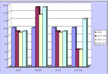
The overall regional price level may be calculated in two alternative ways, either as a weighted index of the composite commodity prices or as regional output prices. We calculated several price measures in order to obtain a robust and consistent picture of the general price level in the region compared to the outside-the-region price level: the net output price, the tradable commodity output price, and the commodity purchase (consumer) price. Given that all three price measures yield similar results, we report only the policy impact on output prices. Figure 3 reports producer prices for the three policy scenarios relative to the base year (1998).
0 20 40 60 80 100 120 140 160
AGR FOOD MAN LOCAL
1998 2007 BR 2007 LS 2007 EU
Figure 3: Changes in output prices in rural region in percent (1998=100)
According to Figure 3, with unchanged agricultural and rural development poli-cies, as assumed in the base run scenario (2007 BR in Figure 3), output prices might develop more favorably for the food processing industry from 1998 to 2007 (see FOOD in Figure 3). These results are mainly driven by the assumption that the expendi-ture share for demand of processed food compared to demand for raw agricultural products will continue to grow until 2007. The sizable increase in relative prices for manufactured food products is also driven by the fact, that food processing industry in CEE is not eligible for the …nancial support from the European Structural Funds and CAP, implying that any increase in production costs are forwarded to consumers in terms of higher output prices.
In contrast, according to our simulation results, relative output prices would de-crease for agricultural, manufacturing and non-tradable goods and services (see AGR, MAN and LOCAL in Figure 3). In the base run scenario, because nominal protection
rates are assumed to stay at their 1998 levels, the regional output prices for tradable goods would change at the same rate as the projected world market prices between 1998 and 2007. The sharp increase in the producer price for non-tradable goods under the EU scenario stems from the …nancial support of the European Structural Funds to locally produced and locally sold goods and services, such as rural tourism (see LOCAL in Figure 3).
Generally, we may conclude that under either scenario the food processing in-dustry would gain most compared to agriculture, manufacturing, as well as locally produced and consumed goods and services. These results are new and have not been reported in the literature before. However, they are in line with macroeconomic studies (e.g. OECD 2000), which point to the growing role of tertiary industries in the CEE accession countries.
6
Conclusions
In this article we have demonstrated that an inter-regional CGE model can be a useful and reliable tool for analyzing regional impacts of changes in global economic conditions and for assessing both inter-regional and inter-sectoral implications of po-tential policy changes even if computational resources are limited and a full range of regional economic data required by a formal CGE analysis are not available.
In our empirical analysis we found that the rural economy of Latvia, which was used as an example for the Central and East European accession countries, might gain most from integration into the EU, if the CAP and EU Structural Fund support measures are implemented immediately but markets are opened only gradually to foreign competition. These results are in line with the fact that market protection in the EU is currently relatively high compared to the CEE accession countries. Given that in the EU agricultural markets are highly protected, above all, rural households might gain from integration into the EU, if the CAP support measures are equally adopted in the CEE accession countries, as we assumed in our simulations.
Although we have been able to account for several important components and adjustment channels of the rural economy in our inter-regional CGE model, it is important to focus future modeling activities on dealing with remaining limiting assumptions and incorporating more externalities that rural economies face. Above all, one should consider market imperfections, transportation costs, and a dynamic rather than static treatment of regional economies. If all this is ensured, then rural development planners will have a reliable planning tool for the ex-post as well as the ex-ante evaluation of regional and rural development policies.
References
[1] Ando, A., Takanori, S. (1997) A Multi-regional Model for China Based on Price and Quantity Equilibrium, in Chatterji M. (ed.), Regional Science Perspectives for the Future. London MacMillan, pp. 326-344.
[2] Armington, P.S. (1969) A theory of demand for products distinguished by place of production, IMF Sta¤ Papers 16, pp. 159–178.
[3] Anselin, M. (1990) Integrated and multi-regional approaches in regional analysis. [4] Azis, I. J. (1997 a) The Relevance of Price-Endogenous Models, in Regional
Science Review, Vol. 19.
[5] Azis, I. J. (1997 b) Impacts of Economic Reform on Rural-Urban Welfare A General Equilibrium Framework, in Review of Urban and Regional Development Studies, Vol. 9, pp. 1-19.
[6] Bandara, J. S. (1991) Computable General Equilibrium Models for Development Policy Analysis in LDCs, in Journal of Economic Survey, Vol. 5.
[7] Chambers, R.G. (1988) Applied Production Analysis, A dual Approach, Cam-bridge.
[8] Chiang, A., C. (1984) Fundamental Methods of Mathematical Economics, Sin-gapore.
[9] Comer, J., Jackson, R.W. (1997) A Note on Adjusting National Input-Output Data for a Regional Table Construction, Journal of Regional Science, Vol. 37, no 1, p. 145.
[10] Deaton, A., Muellbauer, J. (1996) Economics and Consumer Behaviour, Cam-bridge CamCam-bridge University Press.
[11] Dervis, K., de Melo, J., Robinson, S. (1982) General Equilibrium Models for Development Policy, Cambridge Cambridge University Press.
[12] Diewert, W.E, Wales, T.J. (1988) Normalised Quadratic Systems of Consumer Demand Functions, Journal of Business and Economics Statistics, no 6, p. 302-312.
[13] Dimaranan, B.V. and McDougall, R.A. (2000). The GTAP 5: A Large-Scale Data Base Construction Project, GTAP Resource No 1406, Purdue, Centre for Global Trade Analysis, Purdue University.
[14] Drabenstott, M., Meeker, L.G. (1999) Equity for Rural America From Wall Street to Main Street, Economic Review, No 2.
[15] European Commission (1999) Sixth Periodic Report on the Social and Economic Situation and Development of the Regions in the European Union, Brüssel. [16] Ferman, B. (1999) Linking the Global and the Local The Future of Regions,
Cities, and Neighbourhoods, Economic Developmenr Quarterly, Vol. 13, no 3, p. 281.
[17] Gunning W. J., Keyzer, M. A. (1995) Applied General Equilibrium Models for Policy Analysis, in Behrman, J., Srinivasan, T. N. (eds.), Handbook of Develop-ment Economics III. Amsterdam Elsevier Science, pp. 2025-2107.
[18] Harrigan, F., McGregor, P. G. (1989) Neo-classical and Kynesian Perspectives on the Regional Macro-economy A Computable General Equilibrium Approach, in Journal of Regional Science, Vol. 29, no 4, pp. 555-573.
[19] Hertel, T. W. (1985) Partial vs. General Equilibrium Analysis and Choice of Functional Form, in Journal of Policy Modelling, Vol. 7, pp. 281-303.
[20] Hewings, G. J. D., Madden, M. (1995) Social and Demographic Accounting, Cambridge Cambridge University Press.
[21] Isard, W., I. J. Azis, M. P. Drennan, R. E. Miller, S. Salzman, E. Thorbecke (1998) Methods of interregional and Regional Analysis. Ashgate Publishing Com-pany, Aldershot.
[22] Isard, W.; Azis, I., J. (1998) Applied general interregional equilibrium, in Isard, W. et al Methods of interregional and Regional Analysis. Aldershot, p. 334. [23] Johnson, T.G., Scott, J.K. (1997) The Changing Nature of Rural Communities,
Community Policy Analysis Centre Academic Papers, Missouri.
[24] Kilkenny, M. (1993) Rural-Urban E¤ects of Terminating Farm Subsidies, in American Journal of Agricultural Economics, vol. 75, pp. 968-980.
[25] Kilkenny, M. (1995) Operationalising a Rural-Urban General Equilibrium Model uning a Bi-Regional SAM, in Hewings, G. J. D., Madden, M., Social and Demo-graphic Accounting, Cambridge Cambridge University Press.
[26] Koh, Y., Schreiner, D., Shin, H. (1993) Comparisons of Fixed Price and General Equilibrium Models, in Regional Science Perspectives, Vol. 23, no 1, pp. 33-80. [27] Lau, L.J. (1978) Testing and Imposing Monotonicity, Convexy and Quasiconvexy
Constrains, in Fuss, M., McFadden, D. (Eds.) Production Economics, Vol. III, Amsterdam, North Holland, p. 409-453.
[28] Lopez-Bazo, E., Vaya, E., Mora, A.J., Surinach, J. (1999) Regional Economic Dynamics and Convergence in the European union, The Annals of Regional Science, Vol. 33, no 3, p. 343.
[29] Mansur, A., Whalley, J. (1984) Numerical Speci…cation of Applied General Equi-librium Models Estimation, Calibration, and Data, in Scarf, H., Shoven, J. Ap-plied General Equilibrium Analysis, N.Y. Cambridge University Press.
[30] McFadden, D. (1978) The General Linear Pro…t Function, in Fuss, M., McFad-den, D. (Eds.) Production Economics, Vol. III, Amsterdam, North Holland, p. 269-286.
[31] Midmore, P., Harrison-May…eld, L. (1996) Rural Economic Modelling Multi-Sectoral Aproaches, in Midmore, P., Harrison-May…eld, L, Rural Economic Mod-elling, Wallingford.
[32] Nijkamp, P., Rietveld, P., Snickars, F. (1986) Regional and Multiregional Eco-nomic Models A Survey.
[33] OECD (2000) Baltic States - A Regional Assessment, Economic Surveys, Paris. [34] Patridge, M.D., Rickman, D.S. (1998) Regional Computable General Equilib-rium Modelling A Survey and Critical Appraisal, International Regional Science Review, Vol. 21, no 3, p. 205.
[35] Rickman, D. (1992) Estimating the Impacts of Regional Business Assistance Programs Alternative Closures in Computable General Equilibrium Model, in Regional Science, Vol. 71, no 4, pp. 421-435.
[36] Pyatt, G., Round J. I. (1985) Social Accounting Matrices, A Basis for Planning, The World Bank, Washington.
[37] Pons-Novell, J., Viladecans-Marsal, E. (1999) Kaldor’s Laws and Spatial Depen-dence EviDepen-dence for the European Regions, Regional Studies, Vol. 33, no 5, p. 443.
[38] Round, J. I. (1988) Incorporating the International, Regional and Spatial Dimen-sion into SAM Some Methods and Applications, in Harrigan, J. W., McGilvray, J. W., and McNicoll, I. H. (eds.), Environment and Planning, pp. 927-936. [39] Sadoulet, E. de Janvry, A. (1995) Quantitative Development Policy Analysis,
Baltimore John Hopkins University Press.
[40] Scarf, H. E., Shoven J. B. (1984) Applied General Equilibrium Analysis, Cam-bridge University Press, CamCam-bridge.
[41] Schindler, G.R., Israilevich, P.R., Hewings, G.J.D. (1997) Regional Economic Performance An Integrated Approach, Growth and Change, Vol. 27, no 4, p. 131.
[42] Shoven, J. B., Whalley, J. (1992) Applying General Equilibrium, N.Y. Cambridge University Press.
[43] Spencer, J. E. (1988) Computable General Equilibrium Modelling, Trade, Factor Mobility, and the Regions, in Recent Advances in Regional Modelling, London Pion.
[44] Stone, J. R. N. (1954) Linear Expenditure Systems and Demand Analysis An Application to the British Demand, Economic Journal, no. 64, p. 511-527. [45] Takayama, T., Judge, G. G. (1976) Spatial and Temporal Price and Allocation
Models, Amsterdam North Holland.
[46] Treyz, G. I. (1993) Regional Economic Modelling – A Systematic Approach to Economic Forecasting and Policy Analysis. Boston.
[47] Vanhove, N., (1999) Regional Policy A European Approach. Aldershot.
T a b le 1 : A g g re g a te d ru ra l-u rb a n S A M fo r L a tv ia , 1 9 9 8 (M io L V L ) R u ra l re gi o n U rb a n re gi o n T o ta l S ec to rs E x p o rt s F a ct o rs A g en ts C a p it a l S ec to rs E x p o rt s F a ct o rs A g en ts C a p it a l R u ra l — — — — — — — — — — — — — — — — — — — — — — — — — — — — — — — — — — — — — — — — — — — — — S ec to rs 3 0 7 7 2 6 2 9 5 7 9 5 5 2 3 4 4 4 9 5 8 Im p o rt s 4 3 5 8 2 1 8 0 6 9 7 F a ct o rs 1 0 6 5 3 4 5 1 4 1 0 A g en ts 4 4 1 3 7 5 5 2 6 1 9 4 5 C a p it a l 1 6 3 1 5 1 4 1 9 2 U rb a n — — — — — — — — — — — — — — — — — — — — — — — — — — — — — — — — — — — — — — — — — — — — — S ec to rs 7 7 2 4 8 4 9 4 0 7 9 8 1 1 9 0 7 1 9 9 Im p o rt s 1 8 0 1 5 4 0 7 6 0 2 F a ct o rs 1 7 3 8 3 5 1 7 7 3 A g en ts 2 5 5 3 5 4 5 8 9 1 2 4 7 1 3 5 1 8 0 6 C a p it a l 3 2 5 3 2 5 T o ta l 4 9 5 8 6 9 7 1 4 1 0 1 9 4 5 1 9 2 7 1 9 9 6 0 2 1 7 7 3 1 8 0 6 3 2 5 S o u rc e: O w n ca lc u la ti o n s b a se d o n th e C en tr a l S ta ti st ic a l B u re a u o f L a tv ia (C S B ) (2 0 0 0 ) a n d G T A P v .5 d a ta .