A Dissertation by
LIANFU CHEN
Submitted to the Office of Graduate Studies of Texas A&M University
in partial fulfillment of the requirements for the degree of DOCTOR OF PHILOSOPHY
December 2011
A Dissertation by
LIANFU CHEN
Submitted to the Office of Graduate Studies of Texas A&M University
in partial fulfillment of the requirements for the degree of DOCTOR OF PHILOSOPHY
Approved by:
Chair of Committee, Mohsen Pourahmadi Committee Members, Daren B.H. Cline
Suhasini Subba Rao Joel Zinn
Head of Department, Simon J. Sheather
December 2011 Major Subject: Statistics
ABSTRACT
Topics on Regularization of Parameters in Multivariate Linear Regression. (December 2011)
Lianfu Chen, B.S., University of Science & Technology of China; M.S., Texas A&M University
Chair of Advisory Committee: Dr. Mohsen Pourahmadi
My dissertation mainly focuses on the regularization of parameters in the multi-variate linear regression under different assumptions on the distribution of the errors. It consists of two topics where we develop iterative procedures to construct sparse estimators for both the regression coefficient and scale matrices simultaneously, and a third topic where we develop a method for testing if the skewness parameter in the skew-normal distribution is parallel to one of the eigenvectors of the scale matrix.
In the first project, we propose a robust procedure for constructing a sparse esti-mator of a multivariate regression coefficient matrix that accounts for the correlations of the response variables. Robustness to outliers is achieved using heavy-tailedt dis-tributions for the multivariate response, and shrinkage is introduced by adding to the negative log-likelihood 1 penalties on the entries of both the regression coefficient matrix and the precision matrix of the responses. Taking advantage of the hierar-chical representation of a multivariate t distribution as the scale mixture of normal distributions and the EM algorithm, the optimization problem is solved iteratively where at each EM iteration suitably modifiedmultivariate regression with covariance
estimation(MRCE) algorithms proposed by Rothman, Levina and Zhu are used. We propose two new optimization algorithms for the penalized likelihood, called MRCEI and MRCEII, which differ from MRCE in the way that the tuning parameters for the two matrices are selected. Estimating the degrees of freedom when penalizing the
en-tries of the matrices presents new computational challenges. A simulation study and real data analysis demonstrate that the MRCEII, which selects the tuning parameter of the precision matrix of the multiple response using theCp criterion, generally does the best among all methods considered in terms of the prediction error, and MRCEI outperforms the MRCE methods when the regression coefficient matrix is less sparse. The second project is motivated by the existence of the skewness in the data for which the symmetric distribution assumption on the errors does not hold. We ex-tend the procedure we have proposed to the case where the errors in the multivariate linear regression follow a multivariate skew-normal or skew-t distribution. Based on the convenient representation of skew-normal and skew-t as well as the EM algorith-m, we develop an optimization algorithalgorith-m, called MRST, to iteratively minimize the negative penalized log-likelihood. We also carry out a simulation study to assess the performance of the method and illustrate its application with one real data example. In the third project, we discuss the asymptotic distributions of the eigenvalues and eigenvectors for the MLE of the scale matrix in a multivariate skew-normal distri-bution. We propose a statistic for testing whether the skewness vector is proportional to one of the eigenvectors of the scale matrix based on the likelihood ratio. Under the alternative, the likelihood is maximized numerically with two different ways of parametrization for the scale matrix: Modified Cholesky Decomposition (MCD) and Givens Angle. We conduct a simulation study and show that the statistic obtained using Givens Angle parametrization performs well and is more reliable than that obtained using MCD.
ACKNOWLEDGMENTS
I would like to gratefully and sincerely thank my advisor, Dr. Mohsen Pourah-madi, for his excellent guidance, understanding, patience and providing me with an excellent atmosphere for doing research during my graduate studies at Texas A&M University. You opened the door for me to this wonderful statistical world and helped me to build a balanced knowledge in both theory and methodology. The experience to work with you is something that I will be proud of and cherish for the rest of my life. Without your help, I would never have accomplished as much as I have achieved. I would like to thank Dr. Daren B.H. Cline, Dr. Suhasini Subba Rao and Dr. Joel Zinn for their valuable discussions and serving on my committee. A special thanks is owed to my master advisor, Dr. Ruzong Fan, for his encouragement and consistent support.
I would like to thank my parents for their faith in me and allowing me to be as ambitious as I wanted. It was under their watchful eyes that I gained so much drive and ability to tackle challenges head on.
TABLE OF CONTENTS
Page
ABSTRACT . . . . iii
DEDICATION . . . . v
ACKNOWLEDGEMENTS . . . . vi
TABLE OF CONTENTS . . . . vii
LIST OF TABLES . . . . ix
LIST OF FIGURES . . . . xi
CHAPTER I INTRODUCTION. . . . 1
1.1 Multivariate Linear Regression . . . 1
1.2 Estimating B While Ignoring Correlations . . . 3
1.3 Covariance Matrix Regularization . . . 5
1.4 Estimating B While Accounting for Correlations . . . 6
1.5 Overview Structure . . . 7
II SPARSE MULTIVARIATE REGRESSION AND COVARI-ANCE ESTIMATION. . . . 8
2.1 Introduction . . . 8
2.2 Parameter Estimation via Penalized t-likelihood . . . 10
2.3 A Simulation Study . . . 21
2.4 Real Data Analysis . . . 28
2.5 Summary . . . 34
III REGULARIZATION OF MULTIVARIATE REGRESSION WITH SKEW ERRORS . . . . 36
3.1 Introduction . . . 36
3.2 Multivariate Skew-normal and -t Distributions . . . 38
3.3 Penalized Skew-normal and Skew-t Log-likelihoods . . . 43
CHAPTER Page
3.5 A Simulation Study . . . 51
3.6 Real Data Analysis . . . 57
3.7 Summary . . . 60
IV TESTING PROPORTIONALITY OF THE SKEWNESS VEC-TOR AND EIGENVECVEC-TORS OF MULTIVARIATE SKEW-NORMAL DISTRIBUTIONS . . . . 62
4.1 Introduction . . . 62
4.2 Distributions of the Eigenvalues and Eigenvectors . . . 64
4.3 The LR Test Statistic . . . 66
4.4 A Simulation Study . . . 69
4.5 Data Analysis . . . 71
4.6 Summary . . . 72
V CONCLUSIONS, EXTENSIONS AND FUTURE WORK . . . . 74
5.1 Regularization of Parameters in Multivariate Linear Re-gression . . . 74
5.2 Principal Component Analysis of a Skew-normal Variable . 74 REFERENCES . . . . 76 APPENDIX A . . . . 86 APPENDIX B . . . . 88 APPENDIX C . . . . 89 APPENDIX D . . . . 90 VITA . . . . 92
LIST OF TABLES
TABLE Page
1 Model error for the AR(1) error covariance models forp=q= 20, s1 = 0.1 and s2 = 1. Average and standard errors in parenthesis are based on 50 replications withn= 50. Tuning parameters were
selected using a 10x resolution. . . . . 23 2 Model error for the AR(1) error covariance models for p = q =
20, s1 = 0.5 ands2 = 1. Average and standard errors in parenthe-sis are based on 50 replications with n = 50. Tuning parameters
were selected using a 10x resolution. . . . . 24 3 True Positive Rate/True Negative Rate for the AR(1) error
co-variance models averaged over 50 replications;n = 50, p=q= 20, s1 = 0.1 and s2 = 1. Tuning parameters were selected using a 10x
resolution. . . . . 25 4 True Positive Rate/True Negative Rate for the AR(1) error
co-variance models averaged over 50 replications;n = 50, p=q= 20, s1 = 0.5 and s2 = 1. Tuning parameters were selected using a 10x
resolution. . . . . 26 5 The average CPU times (in minutes) over 50 replications when
p=q = 20, s1 = 0.5, ρE = 0.9 ands2 = 1. . . . . 27 6 Estimated coefficient matrix B using MRCEII. . . . . 30 7 Average squared prediction error for each company ×103 based
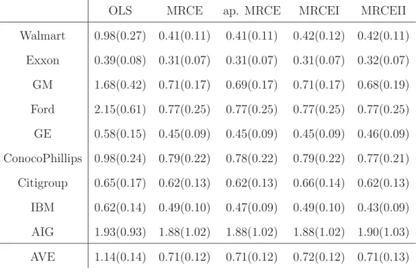
on 26 points. Standard errors are reported in parenthesis. . . . . 31 8 Average squared prediction error for each hour on a day based on
100 points. Standard errors are reported in parenthesis. . . . . 32 9 Proportions of zeros in the estimate of the parameters . . . . 33 10 PE for the AR(1) error covariance with s1 = 0.1, s2 = 1 and
α= (1,1,1,· · · ,1)T. Average and standard errors in parenthesis
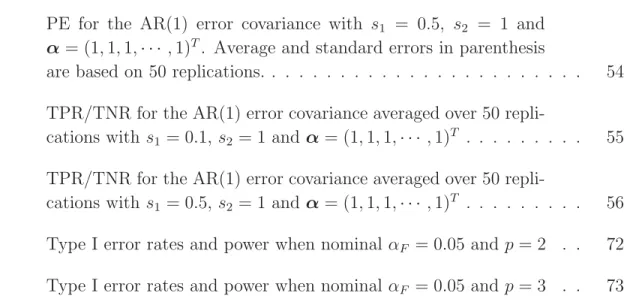
TABLE Page 11 PE for the AR(1) error covariance with s1 = 0.5, s2 = 1 and
α= (1,1,1,· · · ,1)T. Average and standard errors in parenthesis
are based on 50 replications. . . . . 54 12 TPR/TNR for the AR(1) error covariance averaged over 50
repli-cations withs1 = 0.1,s2 = 1 andα= (1,1,1,· · · ,1)T . . . . . 55 13 TPR/TNR for the AR(1) error covariance averaged over 50
repli-cations withs1 = 0.5,s2 = 1 andα= (1,1,1,· · · ,1)T . . . . . 56 14 Type I error rates and power when nominal αF = 0.05 andp= 2 . . 72 15 Type I error rates and power when nominal αF = 0.05 andp= 3 . . 73
LIST OF FIGURES
FIGURE Page
1 Positions of nonzero entries in ˆΩ for different methods applied to
the electricity prices; The straight line indicates the diagonal of ˆΩ. . 34 2 The profile plot of the hourly electricity wholesale prices. The
solid dark curve is the mean profile. . . . . 58 3 The average squared prediction error for each hour on a day based
on 100 points. . . . . 59 4 The estimated skewness parameters using different models and
algorithms (The dash line is the marginal skewness parameter and the solid line is the estimate for α). (a) Lars-lasso without fixing α(b) Lars-lasso with αfixed (c) Cod without fixing α(d)
CHAPTER I
INTRODUCTION
In Statistics, particularly in the fields of machine learning and inverse problems, reg-ularization involves introducing additional information about the parameters in order to solve an ill-posed problem or prevent overfitting. The information usually takes the form of a penalty for complexity such as bounds on the vector norm of the param-eters. From the Bayesian point of view, regularization corresponds to imposing prior distributions on the parameters. In this dissertation, we consider the regularization of parameters in the context of multivariate linear regression where the 1-norm of the parameters is adopted as the penalty.
1.1 Multivariate Linear Regression
The multivariate linear regression is concerned with regressing simultaneously sever-al response variables on the same set of predictor variables. It is commonly used in chemometrics, econometrics, biological and social sciences [1], [2, chap.6] and in the analysis of longitudinal and panel data [3, chap.10]. Specifically, let yi = (yi1,· · · , yiq)T be aq-dimensional response vector andxi = (xi1, xi2,· · · , xip)T be the p predictors for the ith unit. Then, the multivariate linear regression of yi on the covariates xi is of the form
yi =BTxi+i, i = 1,· · · , n (1.1) where B is the p×q regression coefficient matrix and the errors i of dimension q are independent of each other. Let X be the n×p predictor matrix with xTi in its
ith row, Y be then×q response matrix withyTi in its ith row and E be then×q random error matrix with Ti in its ith row. Writing the regression model (1.1) into the matrix form yields the following general linear model:
Y =XB+E. (1.2)
As an example, consider a biochemical data which contain chemical measure-ments on several characteristics of n = 33 individual samples of men’s urine speci-mens. There areq= 5 response variables: pigment creatinine, concentrations of phos-phate, phosphorus, creatinine and choline. The goal was to relate these responses to p= 3 predictors: the weight of the subject, volume and specific gravity. Postulating a multivariate linear regression seems to be a good starting point to analyze the data; see [4] for a recent analysis of the data and suitability of the linearity assumption.
In the multivariate regression, the errors in (1.1) are usually assumed to be independent with mean 0 and covariance matrix Σ. Then, the parameters B and
Σ can be simply estimated by the ordinary least square estimate and the sample covariance matrix of the residuals, respectively, i.e.,
ˆ Bols = (XTX)−1XTY S = 1 n n i=1 (yi−y¯)(yi−y¯)T (1.3) which are the same as their maximum likelihood estimates (MLEs) wheni ∼N(0,Σ) [5]. However, there are some drawbacks for the estimators in (1.3):
(a) The estimators are equivalent to regressing each response on the predictors variables separately [6], so that the estimates may perform suboptimally since they do not utilize the information that the responses are correlated. It is also the case that this type of estimate performs poorly in the presence of outliers, highly correlated response/predictor variables.
(b) For high-dimensional data, particularly when p and q are larger than n, the regression coefficient matrix B can not be estimated using the above formula, since X is not of full column rank. Furthermore, it is known that in this case the sample covariance matrix is a highly unstable estimator of Σ [7], [8]. In these situations, the traditional estimators for B and Σ with pq and q(q+ 1)/2 parameters, respectively, have rather poor performances and are not suitable for prediction and other purposes, so that one must seek workable alternatives based on the idea of regularizing these parameters. Historically, this has been done either individually focusing on B/Σ alone or simultaneously, depending on whether the dependence between the multivariate responses is ignored or not. We briefly review some of these developments in the next three sections.
1.2 Estimating B While Ignoring Correlations
A way to fix some of the pitfalls of the ordinary least squares estimator is to reduce its pq parameters in the regression coefficient matrix B. This can be done either through dimension-reduction techniques such as reduced-rank regression [9], [10], [11], criterion-based model selection methods [12], [13], [14], Bayesian model selection [15], [16], principal components, partial least squares [17], [18] and linear factor regression [19], [20].
Another approach reduces the number of parameters through regularization which may force some entries of B towards zero; see [4] for a review. This ap-proach can be unified and viewed as estimatingB by solving the following constraint optimization problem: ˆ B = arg min B tr(Y −XB)T(Y −XB) subject to: C(B)≤t, (1.4)
whereC(B) is a scalar function of B.
Of course, different constraints will lead to different estimates forB. An early and natural constraint isC(B) = j,kb2jkso that (1.4) reduces to solving a ridge regression problem. The well-known 1-norm constraint, i.e., C(B) = j,k|bjk| leads to the Lasso estimate ofB proposed by [21]. Using the Lagrangian form, this optimization problem takes the form
ˆ B = arg min B tr(Y −XB)T(Y −XB)+λ j,k |bjk| . (1.5)
Also, one may assign different weights to different parameters or use the adaptive Lasso [22] which amounts to setting C(B) = j,kwjk|bjk|, where wjks are chosen adaptively using the data. Some other forms of the constraint function C(B) which seem to make a compromise between the Lasso and the ridge regression are: the Bridge regression [23] takingC(B) =j,k|bjk|γ where 1≤γ ≤2; the elastic-net [24] with C(B) =αj,k|bjk|+ (1−2α)j,kb2jk for α∈[0,1].
Group-wise penalty functions are perhaps more suitable for regularizing the mul-tivariate regression parameters. The first example of its kind is the grouped lasso [4] withC(B) = pj=1(b2j1+· · ·+b2jq)0.5. One could also combine the1 and 2 penalties to form the constraint function C(B) =αC1(B) + (1−α)C2(B) for α∈[0,1] where C1(B) = j,k|b|jk and C2(B) =jp=1(b2j1+· · ·+b2jq)0.5. The first constraint controls
the overall sparsity of the coefficient matrixB and the second imposes a group-wise penalty on the rows of B which controls the number of predictors entering into the multivariate regression model [25].
We note that the constraints mentioned so far introduce sparsity only into the regression coefficient matrixBwithout accounting for the covariance structure of the multivariate responses. In other words, they ignore the q(q+ 1)/2 parameters in Σ whose estimation is a problem of great interest in statistics on its own right.
1.3 Covariance Matrix Regularization
Covariance estimation is an important problem in many areas of statistics dealing with correlated data. It is well-known that the sample covariance matrix performs poorly when the number of variables is large relative to the sample size [7], [8]. A wide range of alternatives to the sample covariance matrix has been developed in the last decade or so which involve regularizing large covariance matrices.
For unordered multivariate data, an early and common approach is the ridge regularization which estimates the covariance matrix by an optimal linear combination of the sample covariance matrix and the identity matrix [8], [26]. Such a regularization ends up shrinking the eigenvalues of the sample covariance matrix, and provides more accurate and well-conditioned covariance estimators. Recently, fast alternative methods have been proposed to construct sparse estimates of the precision matrix by adding to the normal likelihood a lasso penalty on its off-diagonal entries [27], [28], [29], [30], [31]. Other approaches include thresholding [32], [33], SPLICE method [34] and SPACE method [35].
For (time-) ordered data, the regularization usually relies on the modified C-holesky decomposition of the precision matrix Σ−1. It is known that [36] the entries of the Cholesky factor are unconstrained and have interpretation as regression coef-ficients when a variable is regressed on its predecessors. [37] uses a nonparametric method to smooth the Cholesky factor of the inverse covariance along its subdiago-nals, and [38], [39] regularize the precision matrix by applying a lasso and adaptive lasso penalty to the Cholesky factor, respectively. However, imposing sparsity on the Cholesky factor does not necessarily imply sparsity of the precision matrix and the sparsity structure in the Cholesky factor could be sensitive to the order of the re-sponse variables. Other approaches that require a sort of time-order on the variables
are tapering [40] and banding [41].
1.4 Estimating B While Accounting for Correlations
The aforementioned methods consider either the regularized estimation of the re-gression coefficient matrix or that of the covariance matrix. In these situations, the two matrices are usually estimated separately, and the covariance matrix does not contribute much to the prediction accuracy. To improve the predictive power, one must take advantage of the correlations among the multivariate response. However, research in this area is rather scarce and there are only a few papers devoted to this important area. The authors in [1] proposed the Curds and Whey (CW) method which predicts a multivariate response vector with ˜Y = ˆYOLSM where ˆYOLS is the ordinary least square prediction and M is a q×q shrinkage matrix estimated from the data in a manner which exploits the correlation in the responses. [26] relies on the idea of ridge regression, and the authors of [42] present a procedure called scout under the multivariate normal assumption on the response and the predictors, and apply regularization to the inverse covariance of the joint distribution.
Rothman et al.’s multivariate regression with covariance estimation (MRCE) method [43] seems to be the first bona fide regularization approach which construct-s construct-sparconstruct-se econstruct-stimateconstruct-s for both matriceconstruct-s construct-simultaneouconstruct-sly. They add two construct-separate laconstruct-sconstruct-so penalties to the negative normal log-likelihood and minimize the ensuing objective function which, up to a constant, is proportional to
g(B,Ω) = tr 1 n(Y −XB)(Y −XB)Ω −log|Ω|+λ1 j=j |ωjj|+λ2 j,k |bjk|,(1.6)
whereΩ= (ωjj) =Σ−1 and λ1, λ2 are the two tuning parameters to be determined
1.5 Overview Structure
It is well known that the normality assumption is too restrictive as it suffers from the lack of robustness against departures from the normal distribution, particularly when data shows multi-modality and skewness. Therefore, in this dissertation, we assume that the errors in (1.1) have a more general distribution. Following [43], the objective is to construct sparse estimators for the regression coefficient matrix and the scale ma-trix simultaneously in this setup. In Chapter II, we extend the MRCE method to the case where the errors in (1.1) follow a multivariate t distribution for accommodating possible outliers. We construct sparse estimators for both regression coefficient and precision matrices simultaneously by minimizing the resulting penalized likelihood for which two algorithms are developed. We conduct a simulation study to assess the performance of the proposed method and illustrate its application with two real data analysis. In Chapter III, the MRCE is further extended to the cases where the errors have a skew distribution for accommodating for the skewness in the data. In Chapter IV, we focus on the direction of the skew vector and its connection with the principal components of a skew-normal variate. We study the asymptotic distributions for the MLEs of the eigenvalues and eigenvectors of the scale matrix. We also propose a statistic for testing if the skewness parameter is proportional to an0 eigenvector of the scale matrix. In Chapter V, I will discuss some possible extensions and my future work.
CHAPTER II
SPARSE MULTIVARIATE REGRESSION AND COVARIANCE ESTIMATION 2.1 Introduction
Compared to the classical data analysis where the errors in (1.2) are assumed to be normal, handling outliers seems to be a more important problem in the high-dimensional data setup that needs special attention, since in the high-high-dimensional spaces the data tends to be more sparse which implies that every observation can appear as an outlier. Furthermore, the notion of which observations are outliers typ-ically varies between users and problem domains. Thus, the traditional approach of detection and removal of outliers is not a feasible option and the idea of robust data analysis might be more suitable alternative. For handling outliers in high dimensions, one could rely on variety of robust methods such as the M-estimators [44], but we use the family of multivariate t distributions for robust estimation of the regression parameters [45], [46]. This approach is of great practical interest since it allows ac-commodating possible outliers by suitably choosing the tail parameter or the degrees of freedom. An important advantage of this approach to robustness is its explicit statement of the probabilistic setting, leading to a clearer interpretation of the result-s compared to the leresult-sresult-s explicit, result-say, M-estimators. The need for robust procedures is also motivated by the fact that data from heavy-tailed distributions are bound to have some extreme observations, so that the assumption of normality may not be plausible or cannot cope with outliers. Important examples of such phenomenon occur in finance, economics, data network and risk analysis [47], [48]. In such cases, the multivariate t distribution would give a more robust inference and allows one to control aspects of the impact of outliers [46], [49].
In this project, our objective is to construct robust and sparse estimates for the regression coefficient matrix while discounting the outliers and accounting for the dependence structure of the responses simultaneously. To this end, we develop robust versions of the MRCE algorithms when the error vector i in (1.1) follows a multivariatet distribution. This provides an extension of the MRCE method in [43] since the multivariatetdistribution approaches the normal distribution as the degrees of freedom goes to infinity.
Using the hierarchical representation of a multivariatet distribution as the scale mixture of normal distributions and the EM algorithm, the optimization problem is solved iteratively where a central role is played by the MRCE algorithms proposed by [43]. We propose two new optimization algorithms for the penalized likelihood, called MRCEI and MRCEII, which differ in the way that the two tuning parameters for the two matrices are selected. Estimating the degrees of freedom when penalizing the entries of the two matrices presents new computational challenges. The simulation study and real data analysis demonstrate that the MRCEII, which selects the tuning parameter of the precision matrix of the multiple response using the Cp criterion, generally does the best among all methods considered in terms of the prediction error, and MRCEI outperforms the MRCE algorithms when the regression coefficient matrix is less sparse.
The remainder of this chapter is organized as follows. We introduce our method-ology for estimating multivariate regression via penalized t-likelihood in Section 2.2, and present two MRCE-type algorithms to implement it. In Section 2.3, we con-duct a simulation study and compare the performance of our method to the MRCE algorithms. In Section 2.4, we apply our methodology to the datasets of weekly log-returns of nine US stocks, and the electricity spot prices from Australia. A summary and discussion of the results are given in Section 2.5.
2.2 Parameter Estimation via Penalized t-likelihood
In this section, we extend the MRCE algorithms in [43] to the setting where the errors in the multivariate regression have a multivariate t distribution. We provide the details for joint estimation of the regression coefficient and precision matrices of a multivariate regression model using a penalizedt-likelihood with unknown degrees of freedom.
2.2.1 The multivariate t distribution
Aq−dimensional random vectorY = (Y1,· · · , Yq)T has a multivariate t distribution, denoted bytν(μ,Σ), if its probability density function is
f(y;ν,μ,Σ) = Γ ν+q 2 Γν2(νπ)q2|Σ| −1 2 1 + (y−μ) TΣ−1(y−μ) ν −ν+q 2 , (2.1)
whereμ,Σandν are called its location, scale matrix and degrees of freedom, respec-tively. The mean and covariance matrix of the multivariate t distribution are
E(Y) = μ and Cov(Y) = ν
ν−2Σ. (2.2)
whereν should be greater than two for the existence of the covariance matrix. In this project, we rely extensively on the fact that a multivariate t distribution can be represented as a scale mixture of normals with the mixing variable having a Gamma distribution [46]. Specifically, our estimation procedure exploits its hierar-chical representation that if
Y|W =w∼N
μ,w1Σ
and W ∼Gamma(ν/2, ν/2), (2.3) then, the marginal distribution of Y is the multivariate t distribution defined in (2.1) [50].
Unlike the estimates of the parameters of multivariate normal distribution which are vulnerable to the outliers, those of the multivariatetare robust and can handle the outliers or atypical observations, without the need to detecting or removing them. The degrees of freedomν controls the kurtosis or heaviness of the tail of the distribution. Whenν = 1, the distribution corresponds to the q-variate Cauchy distribution which has heavy tails; when ν goes to infinity, the multivariate t distribution approaches the normal distribution with mean vector μ and covariance matrix Σ. See [46] for more discussions on the properties of multivariate t distributions and their roles in robust estimation in variety of situations including the multivariate regression.
2.2.2 The Penalized t-likelihood
We extend the model in (1.1) by assuming that the error i has a multivariate t distribution with mean μ = 0, degrees of freedom ν > 2 and scale matrix Σ. In the following, we also assume that the columns ofX and Y are centered so that the intercept term can be omitted.
Given the covariate matrix X and the response matrix Y, the negative log-likelihood is proportional to L(B,Ω, ν) = −2 log Γ ν+q 2 + 2 log Γ ν 2 +qlogν−log|Ω| + ν+q n n i=1 log 1 + 1 ν(yi−BTxi)TΩ(yi−BTxi) (2.4) whereΩ=Σ−1 is the inverse covariance or precision matrix. We add two 1 penalty terms on the entries of B and Ω to the negative log-likelihood, and estimate both matrices simultaneously by minimizing the penalized log-likelihood:
g(B,Ω, ν) = L(B,Ω, ν) +λ1 j=j |ωjj|+λ2 j,k |bjk|. (2.5)
The lasso penalties onB and Ω encourage sparsity in their estimates and hence can reduce the number of parameters. When the number of predictors is large, such a lasso penalty on the regression coefficient matrix would zero out the irrelevant or redundant predictors and could improve the prediction accuracy. Moreover, in the high-dimensional situations where the empirical sample covariance is singular like whenq > n, the lasso penalty on the precision matrix forces the covariance estimate to be nonsingular and well-conditioned.
Compared to the MRCE algorithms [43], minimization of the penalized negative likelihoodg(B,Ω, ν) is expected to be more complicated. Note that unlike the normal error case, even when λ1 = λ2 = 0 the maximum likelihood estimates of B and Ω do not have closed forms [46]. A fast method for optimization of lasso-type problems is the coordinate descent algorithm [51], but this cannot be applied directly to our problem since the objective function g(B,Ω, ν) is not convex in either B or Ω.
In this section, we propose iterative methods to find the minimizer of the ob-jective function through a sequence of estimators using an Expectation Conditional Maximization (ECM) algorithm [52].
2.2.3 Iterative Optimization Algorithms via ECM and MRCE
Using the conditional Gaussian representation of the multivariate t distribution in (2.3) and the EM algorithm [53], we solve the optimization problem in (2.5) via iterative applications of the MRCE algorithms [43].
2.2.3.1 The EM Algorithm and Penalized t-likelihood
The EM algorithm is an iterative procedure for finding the MLE’s of the parameters in situations where the model depends on some missing or latent variables so that computing the MLE is not straightforward. The EM algorithm alternates between an
expectation (E) step and a maximization (M) step [53]. In the E-step, it computes the expectation of the log-likelihood by replacing the unobservables with their conditional expectations given the current estimates of the parameters and the data; in the M-step, it maximizes the expected log-likelihood calculated in the E-step.
We illustrate the EM algorithms by writing the multivariate t distribution as a scale mixture of normals. LetW1, W2,· · · , Wn be the missing variables such that
i|Wi =wi ∼N(0,Σ/wi), (2.6)
are independent fori= 1,· · · , n, and
W1, W2,· · ·, Wni.i.d∼Gamma ν 2, ν 2 . (2.7)
We augment the data by including the latent variables Wis and treat (yi, wi),1 ≤ i≤ n as the complete data. Hence in this context, the original observations yis are regarded as being incomplete and (2.4) is the negative incomplete-data log-likelihood. The joint distribution of (yi, wi), 1 ≤ i ≤ n, is called the complete-data likelihood and the negative penalized complete-data log-likelihood is proportional to
gc(B,Ω, ν) = −log|Ω|+ 1n n i=1 wi(yi−BTxi)TΩ(yi−BTxi) +a(ν) +λ1 j=j |ωjj|+λ2 j,k |bjk|, (2.8) where a(ν) = 2 log Γ ν 2 −νlog ν 2 − 1 n(ν+q−2) n j=1 logwj + ν n n j=1 wj. (2.9)
The optimization problem ofg(B,Ω, ν) in (2.5) can be solved by iteratively computing the minimizer of gc(B,Ω, ν) in (2.8) via an EM algorithm implemented as follows:
the negative penalized complete-data log-likelihood function in (2.8) given the ob-served data matrix Y and X with the current estimate of the parameters ˆΘ(k) = ( ˆB(k),Ωˆ(k),νˆ(k)).
Since gc(B,Ω, ν) is linear in both wi and logwi, the E-step amounts to simply replacing these by their corresponding conditional expectationsE(Wj|Y,X,Θˆ(k)) and E(logWj|Y,X,Θˆ(k)). Recalling that the gamma distribution is the conjugate prior distribution forWj, then it is not difficult to show that the conditional distribution of Wj given the current estimate ˆΘ(k)and the data (X,Y) is also a Gamma distribution
[52], namely, Wj|Y,X,Θˆ(k) ∼Gamma ν(k)+q 2 , ν(k)+δ(y j,xj; ˆΘ(k)) 2 , (2.10) where δ(yj,xj; ˆΘ(k)) = yj −( ˆB(k))Txj T ˆ Ω(k)yj−( ˆB(k))Txj , (2.11)
is the Mahalanobis distance between yj and ( ˆB(k))Txj. Therefore, from (2.10), we have that u(jk) =E(Wj|Y,X,Θˆ(k)) = νˆ (k)+q ˆ ν(k)+δ(y j,xj; ˆΘ(k)) . (2.12)
To calculate the conditional expectation of logWi, we rely on the fact that if W has a Gamma(α, γ) distribution, then
E(logW) = ψ(α) + logγ,
E-step yields E(logWj|Y,X,Θˆ(k)) = ψ ˆ ν(k)+q 2 −log ˆ ν(k)+δ(y j,xj; ˆΘ(k)) 2 = ψ ν(k)+q 2 −log ν(k)+q 2 + log u(jk). (2.13) See [52] for more details on computing these conditional expectations.
M-step: When all the latent variables are known, the regularization problem
in (2.8) is similar to that considered in [43], except for optimization with respect to ν. However, since the minimization of (2.8) over the whole parameter space is challenging, we replace the M-step with a few Conditional-Maximization (CM) steps listed below.
CM1: Since the degrees of freedom ν is separated from the other parameters, we update it numerically by
ˆ
ν(k+1)= arg min
ν{a(ν)}. (2.14)
CM2: Given B= ˆB(k), solving the optimization problem forΩin (2.8) is equivalent to computing ˆ Ω(k+1) = arg minΩ −log|Ω|+ tr{ΩS(k)}+ λ1 j=j |ωjj| , (2.15) where S(k) = n1 ni=1wi yi−( ˆB(k))Txi yi−( ˆB(k))Txi T
. This is the 1 penalized covariance estimation problem considered in [27], [29], [30] and [31]. We use the fast graphical lasso algorithm in [29] to solve (2.15).
CM3: Given Ω = ˆΩ(k+1), finding the minimizer of gc(B,Ω, ν) with respect to
B is equivalent to minimizing ˜ g(B) = 1 n n i=1 wi(yi−BTxi)TΩˆ(k+1)(yi−BTxi) +λ2 j,k |bjk|, (2.16)
which can be solved using a lasso-type algorithm described next.
Define a long vectorβof lengthpqasβ = (b11, b21,· · · , bp1,· · · , b1q, b2q,· · · , bpq)T andXi =Iq×q⊗xiT, where⊗is the Kronecker product andIq×qis the identity matrix. Consider the Cholesky decomposition of Ω as Ω = LTL, where L is a q×q upper triangular matrix. Let ˜y = √1
n( √w1yT 1LT,√w2yT2LT,· · · ,√wnyTnLT)T which is of lengthqn and ˜X = √1 n( √w1XT
1LT,· · · ,√wnXTnLT)T. Then, (2.16) can be rewritten
more compactly as ˜ g(β) = y˜−X˜β2+λ2 pq j=1 |βj|. (2.17)
This is a quadratic minimization problem subject to a linear constraint on the pa-rameters which is exactly the lasso problem. There are efficient algorithms for solving this problem for all values ofλ; see the homotopy algorithm of [54] and the Lars-lasso algorithm of [55]. Another simpler algorithm for solving this problem for a fixed λ is the coordinate descent algorithm. This algorithm finds the minimizer of (2.17), say ˜
β, by updating each of its coordinates ˜βj, j = 1,· · · , pq, given the others, using ˜ βj =T nq i=1 ˜ xij(˜yi−y˜i(j)),2λ2 , where ˜X = (˜xij), ˜y = (˜y1,· · · ,y˜nq)T, ˜yi(j) = k=jx˜ijβ˜k and T(x, λ) = sgn(x)(|x| − λ)+. Then it cycles through all ˜βjs until convergence.
2.2.3.2 Two MRCE Algorithms with t-errors
In this section, first we summarize the EM algorithm for minimizing(2.8) and refer to it as the MRCEI algorithm. We use the coordinate descent algorithm to solve the lasso regression problem in (2.17). As in [43], j,k|ˆbridgejk | is used to scale the test of convergence in the MRCEI algorithm, where ˆBridge = (XTX+λ2I)−1XTY, and is
the tolerance parameter , set at 10−4 by default.
MRCEI algorithm: With λ1 and λ2 fixed, initialize the parameters Θ = Θ(0).
On the (k+1)th iteration,
E-step: Estimate the latent variablesWiand logWi by their conditional expectations
as in (2.12) and (2.13).
CM1: Estimateν = ˆν(k+1) by numerically minimizing the a(ν) in (3.3).
CM2: UpdateΩ= ˆΩ(k+1) in (2.15) using the graphical lasso algorithm.
CM3: UpdateB= ˆB(k+1) in (2.17) using the coordinate descent algorithm.
Repeat the E- and CM-steps until the estimates of the parameters converge, that is,
j,k|ˆb(jkk+1)−ˆb(jkk)| ≤
jk|ˆbridgejk |.
The MRCEI is an iterative version of the MRCE method of [43], in the sense that it repeats CM2 and CM3 steps until convergence. Compared with the MRCE method, MRCEI is expected to take longer time to converge due to the iterations in the EM algorithm. This means that, just like the MRCE method, applying MRCEI to high dimensional data would be computationally expensive or intractable. In practice, even for smaller p and q, hundreds of iterations for some values of (λ1, λ2) might be needed for the MRCEI algorithm to converge.
As discussed in Section 2.2.4 below, the tuning parameters λ1 and λ2 in MRCEI would be selected via K-fold cross-validation over a grid of values of (λ1, λ2). To reduce the computational cost for choosing the two tuning parameters, we make two modifications in the above algorithm and propose the faster MRCEII algorithm. The key and primary modification is to keep λ1 fixed and λ2 variable. The secondary modification is to replace the coordinate descent algorithm in the CM3 step by the Lars-lasso algorithm.
MRCEII algorithm: For a fixed value ofλ1, initialize the parameters Θ = Θ(0).
E-step: Estimate the latent variablesWiand logWi by their conditional expectations as in (2.12) and (2.13).
CM1: Estimateν = ˆν(k+1) by numerically minimizing a(ν) in (3.3).
CM2: UpdateΩ= ˆΩ(k+1) in (2.15) using the graphical lasso algorithm.
CM3: UpdateB = ˆB(k+1)and the value ofλ2in (2.17) using the Lars-lasso algorithm. Repeat the E- and CM-steps until the estimates of the parameters converge, that is,
j,k|ˆb(jkk+1)−ˆb(jkk)| ≤
jk|˜bridgejk |, where ˜Bridge = (XX+λ1I)−1XY.
In MRCEII, for each value ofλ1, an estimate ofB with a corresponding value of λ2 will be obtained in the CM3 step. When choosing the tuning parameter, one has only to consider a few selected values of λ1, rather than a grid of values of (λ1, λ2). This results in a great reduction of the computational cost so far as iterations are concerned.
2.2.4 Tuning Parameters Selection
For the MRCEI, we consider a grid of values of (λ1, λ2) and choose the tuning param-eters (λ1, λ2) via K-fold cross-validation as the minimizer of an unbiased estimate of the expected prediction error variance described next.
To start, we randomly split the full dataset S = {(xi,yi), i = 1,2,· · · , n} into K subsets of about the same size, denoted by Sk, k = 1,2,· · · , K. For each k, we use S−Sk as the training set to estimate the parameters and Sk as the test set to validate. Then, we select the tuning parameters (λ1, λ2) that minimizes the criterion of mean squared prediction error over allq variables of the response, that is,
(ˆλ1,λ2ˆ ) = arg min (λ1,λ2) 1 Kq K k=1 Y(k)−X(k)Bˆ(λ−1,λk)22L2 , (2.18)
whereY(k),X(k) are the validation response matrix and the predictor matrix formed by the subset Sk, respectively, and ˆBλ1,λ2
MRCEI for the training dataS−Sk.
For the MRCEII, we randomly partition the full dataset S into two subsets, the training set S1 and the validation set S2, and then select the tuning parameters in two steps. In the first step, for each value of λ1, we follow Efron et al. (2004, p. 17) and simply chooseλ2 by the Cp criterion using the training data. That is, λ2 is chosen as the minimizer of the function
λ2 = arg minλ 2>0 RSS ˆ σ2 −n+ 2d , (2.19)
whered is the number of nonzero elements in the estimate of β, RSS is the residual sum of squares of model (2.17) and ˆσ2 is the corresponding estimated variance of the model. At the second step, for each pair of (λ1, λ2) obtained in the first step, we select the one with minimum mean prediction error over allq responses:
(ˆλ1,ˆλ2) = arg min (λ1,λ2) 1 q Y∗−X∗Bˆλ1,λ22 L2 , (2.20)
where ˆBλ1,λ2 is the sparse estimate of B in (2.17) using the Lars-lasso algorithm
for the training set, and Y∗, X∗ are the validation matrices for the responses and predictors, respectively.
In the simulation study and the real data analysis, we select λ1 from some pre-defined set Λ for both MRCEI and II, andλ2 from the same set Λ for MRCEI.
2.2.5 Estimation of The Degrees of Freedom
If the degrees of freedom is known, the CM1 step in the algorithms can be ignored. Otherwise, one should update the estimate of ν via the CM1 step at each iteration. However, in our simulations we have noticed that the estimated sequence{νˆ(k)}using the EM algorithm usually decrease monotonically towards a small positive number less than 2 which is not compatible with the existence of the covariance matrix of a
multivariatetdistribution. This phenomenon which is mostly due to the monotonicity of the likelihood function in the EM algorithm [53] is explained in more details next. Taking the derivative ofa(ν) with respect toν, the optimization problem in (3.3) is equivalent to solving the equation
ψν 2 −log ν 2 + 1 n n j=1 u(jk)−log(u(jk)) −ψ ν(k)+q 2 + log ν(k)+q 2 = 1(2.21) At each iteration, by the monotonicity of the likelihood function in the EM algorithm, the negative penalized likelihood function will decrease and some entries in the two matrices of parameters are forced to be zero. After a few warm-up iterations, for most js the sequences formed by
δ(yj,xj; ˆΘ(k))
k≥1 will decrease. Consequently, the corresponding sequence
u(jk)
k≥1will increase and be greater than 1 which makes the third term in (2.21) to increase, since the functionf(x) =x−log(x) is increasing for x≥ 1. As shown in [52], the function h(x) = ψ(x)−log(x) is strictly increasing over (0,∞), hence the sequenceν(k)
k≥1 obtained from (2.21) will decrease. Finally, the decrease in the third term of (2.21) due to the shrinkage of the parameters makes the estimated degrees of freedom to be a very small number.
Thus, to obtain feasible estimates of the degrees of freedom, in what follows we ignore the CM1 step in our algorithms, and estimate ν separately using a one-dimensional search. Estimation of the unknown degrees of freedom of the t dis-tributions, in general, is an important problem and has been studied by many au-thors: [46], [52] and [56] consider estimation of ν in an EM framework, while [49] and [57] utilize method of moments estimators forν.
2.3 A Simulation Study
2.3.1 Simulation Design and Models
In this section, we compare the performance of our two algorithms with the MRCE and the approximate MRCE (ap. MRCE) algorithms in [43] using a simulation study with a design similar to theirs.
Throughout this section we will have 50 replications, and in each replication a sparse matrixB is generated by the elementwise product of three matrices:
B=W ∗K ∗Q,
where (W)ij ∼ i.i.d N(0,1),(K)ij ∼i.i.d Bernoulli(s1) and each row of Q is either a vector of 1’s or 0’s with a success probability of 1’s equal to s2. Generating B in this way, we expect (1−s2)p predictors to be irrelevant for all q responses, and we expect each predictor to be relevant for s1q of all the response variables. An n×p predictor matrix X with n = 50 is also generated with rows drawn independently from N(0,Σx), where (Σx)ij = 0.7|i−j|, as in Yuan et al. (2007) and Peng et al. (2009b). We consider two models for the scale matrix of the errors as follows,
• AR(1) covariance model with (ΣE)ij =ρ|Ei−j| forρE = 0,0.5,0.7 and 0.9. • Fractional Gaussian Noise (FGN) error covariance model with
(ΣE)ij = 0.5[(|i−j|+ 1)2H −2|i−j|2H + (|i−j| −1)2H] for H = 0.90 and 0.95.
Then each row of the error matrix E is independently drawn from a multivariate t distributiontν(μ,ΣE) and the response matrixY is constructed usingY =XB+E. To save computation time, we independently generate a validation data of the same
sample size n = 50 within each replication to estimate the prediction error for the algorithms as in [43]. This is similar to performing a K-fold cross-validation as in (3.26) for the MRCEI.
2.3.2 Performance Measures
We measure the performance of various methods in terms of the model error as in [27] and [43]. For an estimate of regression coefficient matrix ˆB, the model error is defined as ME( ˆB) = tr ( ˆB−B)Σx( ˆB−B) . (2.22)
The sparsity recognition performance of ˆB is measured by the true positive rate (TPR) as well as the true negatvie rate (TNR) which are defined as
TPR( ˆB,B) = #{(i, j) : ˆbij = 0 and bij = 0} #{(i, j) :bij = 0} , TNR( ˆB,B) = #{(i, j) : ˆbij = 0 and bij = 0}
#{(i, j) :bij = 0} . (2.23) The TPR is the proportion of nonzero elements inBthat ˆBidentifies correctly, while the TNR measures the proportion of zero elements recognized correctly. One should consider them simultaneously since ˆB = 0 always has perfect TNR and the OLS estimate always has perfect TPR.
2.3.3 Results and Discussions
For the AR(1) error covariance model, we consider different combinations ofν,ρE,s1 and s2 from the following ranges: (1) ν= 10,20,40,100,(2) ρE = 0,0.5,0.7,0.9, (3) s1 = 0.1,0.5, and (4)s2 = 1; for the FGN model, we have the same design except that ρE is replaced by the corresponding FGN error covariance model withH = 0.90 and
0.95. Additionally, the tuning parameters for both error covariance models would be selected from the set Λ = {10x : x = 0,±1,· · · ,±5}. Since the conclusions drawn from these two error models are similar, we only report the results for the AR(1) error covariance model here.
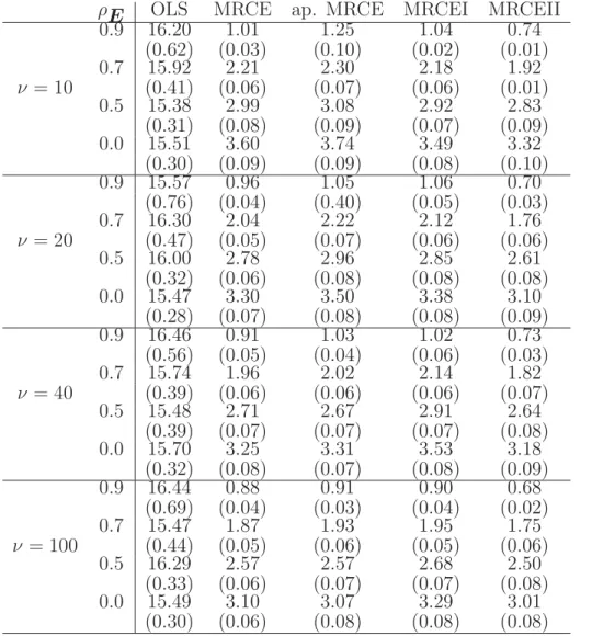
Table 1. Model error for the AR(1) error covariance models for p= q = 20, s1 = 0.1 and s2 = 1. Average and standard errors in parenthesis are based on 50 repli-cations with n= 50. Tuning parameters were selected using a 10x resolution.
ρE OLS MRCE ap. MRCE MRCEI MRCEII
0.9 16.20 1.01 1.25 1.04 0.74 (0.62) (0.03) (0.10) (0.02) (0.01) 0.7 15.92 2.21 2.30 2.18 1.92 ν = 10 (0.41) (0.06) (0.07) (0.06) (0.01) 0.5 15.38 2.99 3.08 2.92 2.83 (0.31) (0.08) (0.09) (0.07) (0.09) 0.0 15.51 3.60 3.74 3.49 3.32 (0.30) (0.09) (0.09) (0.08) (0.10) 0.9 15.57 0.96 1.05 1.06 0.70 (0.76) (0.04) (0.40) (0.05) (0.03) 0.7 16.30 2.04 2.22 2.12 1.76 ν = 20 (0.47) (0.05) (0.07) (0.06) (0.06) 0.5 16.00 2.78 2.96 2.85 2.61 (0.32) (0.06) (0.08) (0.08) (0.08) 0.0 15.47 3.30 3.50 3.38 3.10 (0.28) (0.07) (0.08) (0.08) (0.09) 0.9 16.46 0.91 1.03 1.02 0.73 (0.56) (0.05) (0.04) (0.06) (0.03) 0.7 15.74 1.96 2.02 2.14 1.82 ν = 40 (0.39) (0.06) (0.06) (0.06) (0.07) 0.5 15.48 2.71 2.67 2.91 2.64 (0.39) (0.07) (0.07) (0.07) (0.08) 0.0 15.70 3.25 3.31 3.53 3.18 (0.32) (0.08) (0.07) (0.08) (0.09) 0.9 16.44 0.88 0.91 0.90 0.68 (0.69) (0.04) (0.03) (0.04) (0.02) 0.7 15.47 1.87 1.93 1.95 1.75 ν = 100 (0.44) (0.05) (0.06) (0.05) (0.06) 0.5 16.29 2.57 2.57 2.68 2.50 (0.33) (0.06) (0.07) (0.07) (0.08) 0.0 15.49 3.10 3.07 3.29 3.01 (0.30) (0.06) (0.08) (0.08) (0.08)
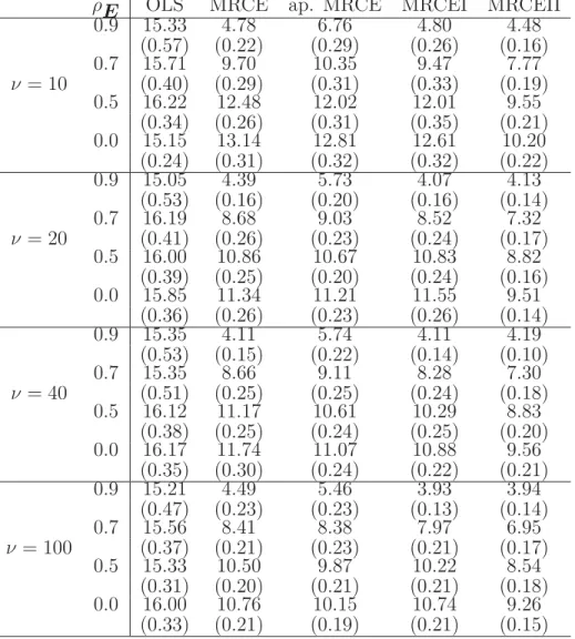
Table 2. Model error for the AR(1) error covariance models for p = q = 20, s1 = 0.5 and s2 = 1. Average and standard errors in parenthesis are based on 50 repli-cations with n= 50. Tuning parameters were selected using a 10x resolution.
ρE OLS MRCE ap. MRCE MRCEI MRCEII
0.9 15.33 4.78 6.76 4.80 4.48 (0.57) (0.22) (0.29) (0.26) (0.16) 0.7 15.71 9.70 10.35 9.47 7.77 ν = 10 (0.40) (0.29) (0.31) (0.33) (0.19) 0.5 16.22 12.48 12.02 12.01 9.55 (0.34) (0.26) (0.31) (0.35) (0.21) 0.0 15.15 13.14 12.81 12.61 10.20 (0.24) (0.31) (0.32) (0.32) (0.22) 0.9 15.05 4.39 5.73 4.07 4.13 (0.53) (0.16) (0.20) (0.16) (0.14) 0.7 16.19 8.68 9.03 8.52 7.32 ν = 20 (0.41) (0.26) (0.23) (0.24) (0.17) 0.5 16.00 10.86 10.67 10.83 8.82 (0.39) (0.25) (0.20) (0.24) (0.16) 0.0 15.85 11.34 11.21 11.55 9.51 (0.36) (0.26) (0.23) (0.26) (0.14) 0.9 15.35 4.11 5.74 4.11 4.19 (0.53) (0.15) (0.22) (0.14) (0.10) 0.7 15.35 8.66 9.11 8.28 7.30 ν = 40 (0.51) (0.25) (0.25) (0.24) (0.18) 0.5 16.12 11.17 10.61 10.29 8.83 (0.38) (0.25) (0.24) (0.25) (0.20) 0.0 16.17 11.74 11.07 10.88 9.56 (0.35) (0.30) (0.24) (0.22) (0.21) 0.9 15.21 4.49 5.46 3.93 3.94 (0.47) (0.23) (0.23) (0.13) (0.14) 0.7 15.56 8.41 8.38 7.97 6.95 ν = 100 (0.37) (0.21) (0.23) (0.21) (0.17) 0.5 15.33 10.50 9.87 10.22 8.54 (0.31) (0.20) (0.21) (0.21) (0.18) 0.0 16.00 10.76 10.15 10.74 9.26 (0.33) (0.21) (0.19) (0.21) (0.15)
Tables 1 and 2 present the results of the simulation study for p = q = 20. We note that, withν fixed, the model errors increase asρE decreases , except for the OLS method. The OLS has by far the largest model errors, indeed, it does the worst among the methods considered. In addition, the MRCEII algorithm generally outperforms the other methods in terms of the model error. This seems to be mostly due to
the alternative method of selecting its tuning parameters. In the MRCEI algorithm, cross-validation is carried out over a grid of points of (λ1, λ2). Therefore, the selected tuning parameter (ˆλ1,λ2ˆ ) is usually a vertex of the rectangle that contains the optimal value. In the MRCEII algorithm, we fix λ1 at some pre-defined points and for each value of λ1, λ2 is selected using the Cp criterion. The tuning parameters selected in this way allowλ2 to move on the edge of the rectangles so that (ˆλ1,λ2ˆ ) is more likely to be closer to the optimal value in (2.20), leading to smaller model errors.
Table 3. True Positive Rate/True Negative Rate for the AR(1) error covariance models averaged over 50 replications; n = 50, p = q = 20, s1 = 0.1 and s2 = 1. Tuning parameters were selected using a 10x resolution.
ρE MRCE ap. MRCE MRCEI MRCEII
0.9 0.92/0.59 0.92/0.61 0.94/0.52 0.92/0.74 ν= 10 0.7 0.87/0.63 0.88/0.64 0.88/0.59 0.85/0.74 0.5 0.84/0.66 0.85/0.65 0.85/0.63 0.82/0.75 0.0 0.82/0.68 0.83/0.66 0.85/0.64 0.81/0.76 0.9 0.93/0.58 0.93/0.61 0.94/0.53 0.92/0.75 ν= 20 0.7 0.90/0.61 0.89/0.62 0.89/0.60 0.86/0.76 0.5 0.87/0.64 0.86/0.64 0.86/0.63 0.83/0.76 0.0 0.85/0.65 0.84/0.66 0.84/0.63 0.80/0.77 0.9 0.94/0.58 0.94/0.62 0.93/0.55 0.91/0.75 ν= 40 0.7 0.90/0.61 0.87/0.63 0.88/0.60 0.86/0.74 0.5 0.87/0.63 0.89/0.63 0.85/0.63 0.82/0.75 0.0 0.84/0.64 0.85/0.65 0.83/0.64 0.79/0.78 0.9 0.93/0.58 0.92/0.60 0.92/0.56 0.91/0.73 ν = 100 0.7 0.89/0.61 0.87/0.63 0.88/0.60 0.87/0.75 0.5 0.87/0.63 0.85/0.63 0.85/0.62 0.84/0.75 0.0 0.85/0.64 0.82/0.65 0.83/0.63 0.82/0.77
particular, the MRCEI has comparable performance to MRCEII whenν = 20,40 or 100 with highly correlated errors (ρE = 0.9). For the more sparse coefficient matrix
B (s1 = 0.1), when ν is small, the MRCEI tends to have smaller model errors than the MRCE and ap. MRCE. However, when ν becomes large, they outperform the MRCEI even though the fitted model is incorrect. This is because asνgoes to infinity the multivariatet approaches the normal distribution for which the MRCE and ap. MRCE have outstanding performance for a sparserB.
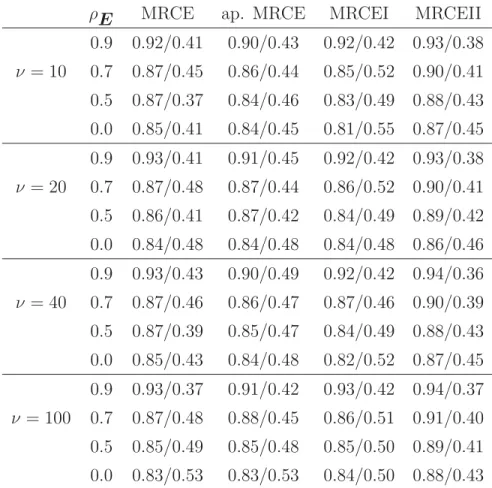
Table 4. True Positive Rate/True Negative Rate for the AR(1) error covariance models averaged over 50 replications; n = 50, p = q = 20, s1 = 0.5 and s2 = 1. Tuning parameters were selected using a 10x resolution.
ρE MRCE ap. MRCE MRCEI MRCEII
0.9 0.92/0.41 0.90/0.43 0.92/0.42 0.93/0.38 ν= 10 0.7 0.87/0.45 0.86/0.44 0.85/0.52 0.90/0.41 0.5 0.87/0.37 0.84/0.46 0.83/0.49 0.88/0.43 0.0 0.85/0.41 0.84/0.45 0.81/0.55 0.87/0.45 0.9 0.93/0.41 0.91/0.45 0.92/0.42 0.93/0.38 ν= 20 0.7 0.87/0.48 0.87/0.44 0.86/0.52 0.90/0.41 0.5 0.86/0.41 0.87/0.42 0.84/0.49 0.89/0.42 0.0 0.84/0.48 0.84/0.48 0.84/0.48 0.86/0.46 0.9 0.93/0.43 0.90/0.49 0.92/0.42 0.94/0.36 ν= 40 0.7 0.87/0.46 0.86/0.47 0.87/0.46 0.90/0.39 0.5 0.87/0.39 0.85/0.47 0.84/0.49 0.88/0.43 0.0 0.85/0.43 0.84/0.48 0.82/0.52 0.87/0.45 0.9 0.93/0.37 0.91/0.42 0.93/0.42 0.94/0.37 ν = 100 0.7 0.87/0.48 0.88/0.45 0.86/0.51 0.91/0.40 0.5 0.85/0.49 0.85/0.48 0.85/0.50 0.89/0.41 0.0 0.83/0.53 0.83/0.53 0.84/0.50 0.88/0.43
error model are also reported in Tables 3 and 4. We note that, with the degrees of freedom ν fixed, as ρE decreases, the true positive rates tend to decrease while the true negative rates tend to increase. Moreover, the MRCE methods and MRCEI have comparable true positive and negative rates, so the comparison among them should be based on the model errors. The MRCEII also has comparable true positive rates with the other methods, but its true negative rates are substantially greater whenB is sparser. Along with the substantially smaller prediction errors, the MRCEII has an excellent performance when B is sparser. When the coefficient matrix B is not so sparse, MRCEII seems to be conservative in the sense that it gives a slightly less parsimonious estimate ofB than other methods.
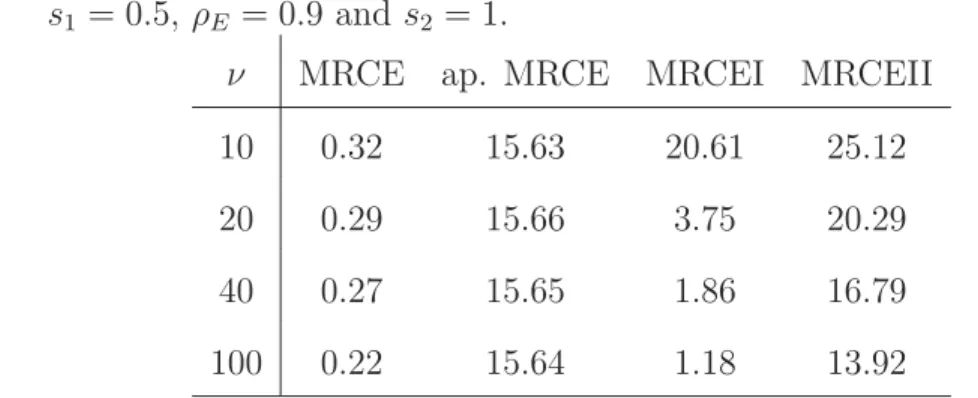
We report the average CPU times in Table 5 over 50 replications whenp=q= 20, s1 = 0.5, ρE = 0.9 and s2 = 1 with ν varying from 10 to 100. All computations were carried out on a quad-core Intel Xeon 2.5 GHz processor with 10GB of RAM. The MRCEI algorithm is faster than the MRCEII for larger ν, because in this situation the MRCEI algorithm takes fewer EM iterations to converge.
Table 5. The average CPU times (in minutes) over 50 replications when p =q = 20, s1 = 0.5, ρE = 0.9 ands2 = 1.
ν MRCE ap. MRCE MRCEI MRCEII
10 0.32 15.63 20.61 25.12
20 0.29 15.66 3.75 20.29
40 0.27 15.65 1.86 16.79
2.4 Real Data Analysis
In this section, we illustrate our methods by applying them to two real financial datasets and compare the results with those using the two MRCE methods.
2.4.1 Predicting Asset Returns
The first real data example we consider is the weekly log-returns of stocks of 9 large American companies in 2004, which was also analyzed in [27] and [43]. Following their approaches, we fit a VAR(1) (vector autoregression of order 1) model to the data:
yt=BTyt−1+t,1≤t≤T, (2.24)
whereyt is the vector of log-returns of the stocks in week t. Writing (2.24) into the matrix form as
YT =YT−1B+E, (2.25)
where YT = (yT2,y3T,· · · ,yTT)T and YT−1 = (yT1,yT2,· · · ,yTT−1)T makes it a special case of the multivariate linear regression model (1.2). In [43], it is assumed that the error in (2.25) has a multivariate normal distribution and apply the MRCE method, but there is ample empirical evidence in the finance literature that the asset returns often exhibit heavy-tails.
We model the asset returns data using the multivariatet distribution which has proved successful in handling the heavy-tailed data in such applications [58], [59]. The MLE of the degrees of freedom is ˆν = 10.15 using the log-returns data for the whole year. The other parameters in the model are estimated using the log-returns of the stocks for the first half of the year (T=26) as the training set, and the rest
as the test set. The tuning parameters are selected from the set Λ = {2x : x = −25,−24,· · · ,10}. For the MRCEI algorithm, we select the tuning parameters via a 10-fold cross-validation; for the MRCEII, we use the last 10% of the log-returns of the first half year as the validation data and the remaining 90% as the training data. The estimated coefficient matrix ˆB using MRCEI turns out to be zero or a fully sparse estimate, compared with the MRCE and ap. MRCE estimates which have 4/81 and 12/81 nonzero coefficients, respectively. However, the MRCEII estimate of
B reported in Table 6, has 19 nonzero entries, and there are 22 zeros in the estimate of Ω. The MRCEII, MRCE and ap. MRCE have four common nonzero entries at the positions (1,7),(4,1),(4,2) and (4,8) of B. This suggests, for example, the log-returns for Walmart at week t-1 as a relevant predictor for the Citigroup at week t, and the log-returns for Ford at week t-1 as a relevant predictor of Walmart, Exxon and GM at week t.
We evaluate the predictive performance by the average squared prediction error for each company over the data from the second half of the year, the result is reported in Table 7. Except for OLS, other methods have comparable performance in terms of the prediction error, though still the MRCEII is slightly better than the other methods. This finding is consistent with the results of our simulation study. In addition, the MRCEI estimating a null model for the data indicates that the signal from the predictors in this example is relatively weak.
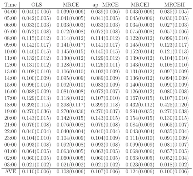
2.4.2 Intraday Electricity Prices
Next, we apply our method to the hourly average electricity spot prices collected in the Australian state of New South Wales (NSW) from July 2, 2003 to June 30, 2006, starting at 04:00 and ending at 03:00 each day. The dataset consists of 26352 obser-vations during a period of T = 1098 days and was previously analyzed in [60] using
Table 6. Estimated coefficient matrix B using MRCEII.
Wal Exx GM Ford GE CPhi Citi IBM AIG
Wal 0 0 0 0 0 0 0.2289 0.2287 0 Exx 0 0 0 0 0 0 0 -0.1168 0 GM 0 0 0.0237 0 0 0 0 0 -0.0574 Ford -0.1639 0.0336 0 0 0.0092 0 0 -0.0834 0 GE 0 0 0 0 0 0.133 -0.0125 0.0662 0 CPhi 0 0.0505 0 0 0.0597 0 -0.0458 0 0 Citi 0 -0.0101 0.0923 0 0 0 0 0 0 IBM 0 0 0 0 0 0 0 0 0 AIG 0 0 0.0306 0 0 0 -0.0564 0 0
a Bayesian method and skew-t distribution for the data. Unlike other commodity prices, most electricity spot prices exhibit trend, strong periodicity, intra-day and inter-day serial correlations, heavy tails, skewness and so on; see [60], [61], [62], [63] for some empirical evidence. As in [60], we consider the vector of the log spot prices at hourly intervals during a day as the response vector with q = 24. The exoge-nous variables which may have effects on the spot prices as the predictors include a simple linear trend, dummy variables for day types (in total 13 dummy variables, representing the seven days of the week and some idiosyncratic public holidays) and eight seasonal polynomials (high order Fourier terms) for a smooth seasonal effect.
Instead of assuming that the covariate effects are the same at all hours within a day as in [60], we fit a multivariate regression model to the log electricity prices by