MOLECULAR-DYNAMICSSIMULATIONS
USINGSPATIALDECOMPOSITION ANDTASK-BASEDPARALLELISM
by
CHRIS MANGIARDI
A thesis submitted in partial fulfilment of the requirements for the degree of
Master of Science (MSc) in Computational Sciences
The Faculty of Graduate Studies Laurentian University Sudbury, Ontario, Canada
c
THESIS DEFENCE COMMITTEE/COMITÉ DE SOUTENANCE DE THÈSE Laurentian Université/Université Laurentienne
Faculty of Graduate Studies/Faculté des études supérieures
Title of Thesis
Titre de la thèse Molecular-Dynamics Simulations using Spatial Decomposition and Task-Based Parallelism
Name of Candidate
Nom du candidat Mangiardi, Christopher Degree Diplôme Master of Science
Department/Program Date of Defence
Département/Programme Computational Sciences Date de la soutenance May 30, 2016
APPROVED/APPROUVÉ
Thesis Examiners/Examinateurs de thèse:
Dr Ralf Meyer
(Supervisor/Directeur(trice) de thèse)
Dr. Lorrie Fava
(Committee member/Membre du comité)
Dr. Aaron Langille
(Committee member/Membre du comité)
Approved for the Faculty of Graduate Studies Approuvé pour la Faculté des études supérieures Dr. Shelley Watson
Madame Shelley Watson
Dr. Mark Wachowiak Dean, Faculty of Graduate Studies (External Examiner/Examinateur externe) Doyenne ntérimaire, Faculté des études supérieures
ACCESSIBILITY CLAUSE AND PERMISSION TO USE
I, Christopher Mangiardi, hereby grant to Laurentian University and/or its agents the non-exclusive license to archive and make accessible my thesis, dissertation, or project report in whole or in part in all forms of media, now or for the duration of my copyright ownership. I retain all other ownership rights to the copyright of the thesis, dissertation or project report. I also reserve the right to use in future works (such as articles or books) all or part of this thesis, dissertation, or project report. I further agree that permission for copying of this thesis in any manner, in whole or in part, for scholarly purposes may be granted by the professor or professors who supervised my thesis work or, in their absence, by the Head of the Department in which my thesis work was done. It is understood that any copying or publication or use of this thesis or parts thereof for financial gain shall not be allowed without my written permission. It is also understood that this copy is being made available in this form by the authority of the copyright owner solely for the purpose of private study and research and may not be copied or reproduced except as permitted by the copyright laws without written authority from the copyright owner.
Abstract
Molecular Dynamics (MD) simulations are an integral method in the computational studies of materials. This thesis discusses an algorithm for large-scale MD simulations using modern multi-and many-core systems on distributed computing networks. In order to utilize the full processing power of these systems, algorithms must be updated to account for newer hardware, such as the many-core Intel Xeon Phi co-processor.
The hybrid method is a data-parallel method of parallelization which combines spatial decom-position using the Message Passing Interface (MPI) to distribute the system onto multiple nodes, along with the cell-task method used for task based parallelism on each node. This allows for the improved performance of task based parallelism on single compute nodes in addition to the benefit of distributed computing allowed by MPI.
Results from benchmark simulations on Intel Xeon multi-core processors, and Intel Xeon Phi coprocessors are presented. Results show that the hybrid method provides better performance than either spatial decomposition or cell-task methods alone on single nodes, and that the hybrid method outperforms the spatial decomposition method on multiple nodes, on a variety of system configurations.
Acknowledgements
This work was made possible by the facilities of the Shared Hierarchical Academic Research Computing Network (SHARCNET:www.sharcnet.ca) and Compute/Calcul Canada.
Computations were made on the supercomputer Guillimin from McGill University, managed by Calcul Québec and Compute Canada. The operation of this supercomputer is funded by the Canada Foundation for Innovation (CFI), NanoQuébec, RMGA and the Fonds de recherche du Québec - Nature et technologies (FRQ-NT).
A special thank you to Aaron Langille, for the constant nagging for me to get my work done. Told you I’d put you in here.
To Lorrie Fava for taking the time to review this work, and for the suggestions.
To Dr. R. Meyer, whose experience and knowledge helped me through many problems along the way. If not for his support, and the opportunity he’s given me, this work would not have been possible.
Contents
1 Introduction 1
2 Background 3
2.1 Main Computational Tasks . . . 4
2.2 Traditional Parallelization Methods . . . 6
2.2.1 Particle Decomposition . . . 6 2.2.2 Force Decomposition . . . 6 2.2.3 Spatial Decomposition . . . 7 2.2.4 Cell-Task Method . . . 8 2.3 Interaction Potentials . . . 10 2.3.1 Lennard-Jones Potential . . . 10 2.3.2 Tight-Binding Potential . . . 11 2.3.3 Mendelev Potential . . . 11 2.4 Related Work . . . 13 3 Methodology 15 3.1 Simulation Program . . . 16
3.2 Spatial Decomposition and the Message Passing Interface . . . 17
3.3 Task-Based Parallelism and Intel Threading Building Blocks . . . 19
3.4 Simulation Configurations . . . 20
3.4.1 Copper (Cu) Systems . . . 21
3.4.2 Iron (Fe) System . . . 23
3.4.3 Silver (Ag) System . . . 24
3.5 Hardware . . . 25
3.5.1 Intel Xeon Phi . . . 26
3.6 Implementation . . . 31
3.6.1 The Outer Grid . . . 33
3.6.2 Force Calculations . . . 37
3.7 Analysis . . . 40
3.7.1 Expectations . . . 41
4 Single Node Results 43 4.1 Multi-Core Processor Results . . . 45
4.2 Xeon Phi Processor Results . . . 50
5 Multi Node Results 56 5.1 Multi-Core Processor Results . . . 58 5.2 Xeon Phi Processor Results . . . 63 5.3 Symmetric Mode Results . . . 68
6 Discussion 70
7 Conclusion 76
List of Tables
3.1 Brief overview of the systems’ hardware. . . 25
3.2 Intel Xeon Phi Extended Math Unit Latency and Throughput. . . 28
4.1 Summary results utilizing a single multi-core processor . . . 48
4.2 Summary results utilizing a single Xeon Phi Processor . . . 53
5.1 Summary results utilizing two Multi-Core Nodes . . . 62
5.2 Summary results utilizing four multi-core nodes . . . 62
5.3 Summary results utilizing two Xeon Phi Processors . . . 64
5.4 Summary results ofCu(spheres)systems utilizing Xeon Phi Processors . . . 65
5.5 Summary results ofCu(honeycomb)systems utilizing Xeon Phi Processors . . . . 66
5.6 Summary results utilizing Symmetric Mode . . . 68
6.1 Parallel efficiency comparison of communication protocols . . . 72
List of Figures
3.1 Cu63 bulk copper system . . . 21
3.2 Cu(porous)copper system . . . 22
3.3 Cu(spheres)copper system . . . 23
3.4 Cu(honeycomb,2x4)copper system . . . 23
3.5 Ag(liquid)silver system . . . 24
3.6 Intel Xeon Phi Core Micro-architecture. . . 26
3.7 Intel Xeon Phi Core Pipeline Stages. . . 27
3.8 Intel Xeon Phi Vector Pipeline Stages. . . 28
3.9 Spatial Decomposition division of theCu(porous)system . . . 31
3.10 Hybrid division of theCu(porous)system . . . 32
4.1 Cu63 results on single multi-core processor . . . 45
4.2 Cu(porous)results on single multi-core processor . . . 47
4.3 Ag(liquid)results on single multi-core processor . . . 49
4.4 Cu63 results on single Xeon Phi processor . . . 51
4.5 Cu126 results on single Xeon Phi processor . . . 52
4.6 Cu(porous)results on single Xeon Phi processor . . . 54
4.7 Ag(liquid)results on single Xeon Phi processor . . . 55
5.1 Cu63 Results on Four multi-core Nodes . . . 59
5.2 Cu105 Results on Two multi-core Nodes . . . 60
5.3 Cu(porous)Results on Four Multi-Core Nodes . . . 61
List of Algorithms
3.1 Pseudo-code of the creation of the inner grid for the cell task parallelism method . 33 3.2 Pseudo-code of the creation of the inner and outer grids for the hybrid parallelism
method . . . 36 3.3 Pseudo-code of the force calculations of many-body potentials for the cell task
method . . . 38 3.4 Pseudo-code of the force calculations of many-body potentials for the hybrid method 39
Chapter 1
Introduction
Molecular dynamics is a computer simulation method that is widely used in computational physics, chemistry and material sciences. The method is described in detail by Allen and Tildesley [1], and Frenkel and Smit [2]. Since molecular dynamics is frequently used to perform large-scale simu-lations on high-performance computers, it is important to develop molecular dynamics algorithms that make the best use of modern computing architectures.
Molecular dynamics simulations compute the trajectories of a set of interacting particles. This requires a model for the forces (or interactions) between particles. The simulation is able to exam-ine interactions between small items such as atoms, or large items such as planets, so long as an appropriate interaction model is supplied. If a short-range force model is used and the simulated system is sufficiently homogeneous, the spatial decomposition method [3] provides an effective means for the parallelization of the simulations. For inhomogeneous systems, an alternative par-allelization scheme named the cell-task method has recently been proposed for shared-memory systems [4, 5, 6].
This thesis discusses a hybrid method that uses a two-level approach for the parallelization of molecular dynamics simulations. The first level is based on the spatial decomposition method and is implemented with the Message-Passing Interface (MPI) [7]. The second parallelization level employs the cell-task method for the parallelization of the workload within the spatial domains
and is implemented with Intel’s Threading Building Blocks Library [8].
The primary rationale for the implementation of the hybrid method is that it extends the range of the cell-task method to more than one compute node. However, even on a single node, the hybrid approach can be advantageous. While the cell-task method is more efficient for inhomoge-neous systems, the situation is less clear for homogeinhomoge-neous systems where spatial decomposition works well. In this case, the situation depends on system details since the overhead of the task management in the cell-task method competes with the communication overhead of the spatial decomposition method. Further, the spatial decomposition approach may have a slight advantage through a more localized memory access pattern. A hybrid approach can lead to performance enhancements as it allows the use of both the cell-task method and spatial decomposition.
This thesis examines the hybrid approach, and compares it to the spatial decomposition and cell-task methods, in order to gauge the performance gains. This is important within molecular dy-namics simulations, in order to reduce the amount of time required to simulate ever larger systems, without the need to wait weeks, or months for the results.
This simulation code used in this thesis to implement the hybrid method has previously been used in several research projects and run for many millions of CPU hours. Some examples of simulations running for weeks or months are described in [9, 10, 11]. The purpose of this work is to take a simulation, and through hybridization improve the performance in order to reduce the overall running time of the simulation. Not only is hybridization relevant to the simulation being worked on, it can also be expanded to other fields, such as computationally expensive simulations, image processing, and many other areas.
Chapter 2
Background
This chapter will introduce some background information on molecular dynamics simulations. This will include
• the main computational tasks, • traditional parallelization methods, • interaction potentials, and
2.1
Main Computational Tasks
Molecular dynamics simulations employ three main computational tasks which account for the largest portion of time spent within the simulation. These tasks include
• the update of particle positions and velocities, • the calculation of forces on particles, and
• for short range forces, the calculation and construction of neighbour lists.
These tasks account for roughly 90% of the time spent in a molecular dynamics simulation, with the force calculations taking the most amount of time out of the three, as determined by using performance profiling on a single core. The update of particle positions and velocities as well as the force calculations are completed at every time step, however the construction of neighbour lists is only done after a specified number of time steps.
Molecular dynamics simulations integrate Newton’s equations of motion in order to calculate the trajectories of particles. By taking advantage of Newton’s third law of motion, which states that for every exuded force there’s an equal and opposite force applied, the number of calculations can effectively be cut in half. In molecular dynamics simulations, a particle’s neighbours consist of nearby particles which exude a force upon the particle. The force calculated on a particle by one of its neighbouring particles can be applied as a negative force to the neighbour.
Molecular dynamics simulations must calculate the forces on particles within the simulation system in order to calculate the velocity and position of each particle. For molecular dynamics simulations, these forces can be calculated using different interaction potentials, described in sec-tion 2.3. For short range forces, a particle’s force upon another is considered to be zero once the distance between particles exceeds a certain point. Depending upon the interaction potential used, the force between particles may approach zero as the particles get to this specified distance, or a sharp cut-off may be used where the force simply drops to zero at the specified distance. The force calculation process is described in section 3.6.2.
Neighbour lists are created by selecting a particle and looping over all other particles and determining if that particle is within a certain range. This distance is slightly larger than the specified cut-off for short range forces as the neighbour lists are not rebuilt at every time step. This allows for particles which move within range of another particle’s range of influence to have an effect on each other, and reduces the need to rebuild the neighbour lists at every time step. This must be completed for all particles within the simulation. For optimization purposes, if a particle iis in the neighbour list of particle j then particle j will not be in the neighbour list of particle i, since by taking advantage of Newton’s third law the calculations of forces are only required on one particle which updates the other particle.
2.2
Traditional Parallelization Methods
Several techniques currently exist for the parallelization of molecular dynamics simulations. Each method is similar in that they each attempt to distribute the workload in order to improve the performance of the simulation, but differ in key aspects. These differences offer advantages and disadvantages to the different parallelization techniques. This section will briefly introduce each parallelization technique, and their advantages and disadvantages.
2.2.1
Particle Decomposition
Particle decomposition is a method which divides the particles within the simulation system evenly amongst the available processing nodes [3]. Each node is then responsible for updating positions, calculating forces, and updates of their own particles. This has an advantage of an even distribution of particles between nodes on any type of simulation system, and helps to improve the performance and results in good load balancing.
This parallelization technique, however, does not guarantee that particles and their neighbours are on the same node. This therefore requires additional communication between nodes in order to transfer all relevant data required to perform the simulation accurately, although typically all positions are broadcast to all nodes. This additional communication causes processing overhead which can degrade the performance of the simulation.
2.2.2
Force Decomposition
Force decomposition is different than most traditional parallelization techniques of decomposition. Instead of dividing the system by particles, the system is partitioned into a block matrix [3]. Since forces must be calculated on all particles in the system, the forces can be written as a matrix F where each element Fi j is the force of particle j on particlei. This matrix can then be blocked into sub-matrices and each block can be distributed to a compute node, which calculates the forces contained within its block of the matrix.
Force decomposition has an advantage of removing some communication between nodes, as each node only requires knowledge of the particles which they process, although since particles can appear on multiple nodes there is still some required communication. This method tends to work well for long range forces where the other decomposition methods would require an excessive amount of communication.
Conversely, it would be difficult for the force decomposition method to take advantage of New-ton’s third law, and hence would require more computations. While simulations can be optimized for this, it would require increased communication between nodes, which takes away from its advantages.
2.2.3
Spatial Decomposition
The spatial decomposition [3] method involves decomposing the simulation system into the num-ber of spatial domains specified, which represent three-dimensional sections of the simulated sys-tem, and are processed by individual compute nodes. These domains are of equal physical size and shape to each other, and the method can be applied in thex,y, andzdirections.
Throughout the simulation, in order to maintain accuracy, information must be communicated between the compute nodes. This information includes, but is not limited to, the particle locations, velocities, and accelerations. This information is used by other spatial domains to compute the forces applied on its own particles which interact with particles in neighbouring domains. Further, the entire particle must be transmitted to another compute node once the particle leaves that node’s spatial domain.
This type of decomposition works well with short range forces as particles and their neighbours are generally contained within the same spatial domain, and hence on the same compute node. Particles which appear near the borders of such spatial domains, however, will have particles in neighbouring domains and hence those particles’ information will need to be exchanged. This is generally a minimal amount of communication compared to particle or force decomposition, although as more domains are added, the amount of data communicated is also increased. This is
offset, however, by the further parallelization of the simulation.
For systems which have uneven distributions of particles, spatial decomposition may perform poorly. As particles are distributed to processors based upon their location within the simulation system, if certain spatial domains contain fewer particles than others, then a load imbalance will occur, which can degrade the performance of the simulation.
2.2.4
Cell-Task Method
System-level thread pool parallelization implementations can use basic approaches, such as parallel for loops, or more advanced parallelization techniques such as task based parallelism. An inherent problem with parallelization of a molecular dynamics simulation using threading is race conditions. Race conditions occur when two or more threads are attempting to update a single particle’s data. This can be avoided by using criticalsections oratomic updates; however, these methods would require thread blocking, which often degrades the performance of the system.
Throughout this work, a task is used to describe small portions of the simulation system which require processing in order to calculate the forces on particles which occur within those portions. These portions of the simulation system are made up of one or more cells, which are sub-domains of the full simulation system, typically the width of the specified cut-off distance. These tasks are used to calculate the forces on the particles and to construct neighbour lists.
The cell-task method [4] avoids this issue by using a dynamic scheduling algorithm which schedules tasks in a fashion which prevents two tasks which contain the same particles from run-ning simultaneously. In order to reduce the number of cores waiting for work, the simulation system is split into thousands of smaller tasks, which allows for several hundred tasks to run si-multaneously without causing cache coherency issues. This method is highly dependent upon short-range interactions for the purposes of building the task lists. Details of this process are de-scribed by Meyer [4].
Since the dynamic scheduler prevents two tasks which access the same particle from running simultaneously, critical sections can be avoided. In order to avoid the load-balancing issue which
can occur with spatial decomposition, this method’s dynamic scheduler will automatically run the next available task once a previous task is complete. Further, tasks which have no particles within can simply be skipped. Despite these advantages, in order for the system to remain accurate, the task lists must be updated when the neighbour-lists are rebuilt, which adds overhead to the process. This method’s dynamic scheduler works well for inhomogeneous systems due to its automated load balancing. However, this method has a disadvantage of requiring the creation of the dynamic scheduler, which is an intensive process. Further, this method is limited to a single compute node due to its use of thread pool parallelization.
2.3
Interaction Potentials
This section will briefly describe the three interaction potentials used for this work. Each of the potentials offers varying degrees of processor and memory strain, and are each therefore important to test with, to determine where limitations may lie.
E
i=
F
∑
i6=jρ
(
r
i j)
!+
1
2
i∑
6=jφ
(
r
i j)
(2.1)
The interaction models follow a general pattern for the interactions of particles which can be found in the embedded atom method (EAM), which is shown in Equation 2.1 [12]. While none of the potentials used throughout this work use EAM, the format remains the same.
2.3.1
Lennard-Jones Potential
The Cutted Lennard-Jones potential is used for a silver system in this work. This potential is the simplest potential used, with reduced calculations involvingφ, which is shown in Equation 2.2.
φ
(
r
i j) =
4
ε
×
σ r 12−
σ r 6+
c
if
r
≤
r
cut0
if
r
>
r
cut(2.2)
In this, ε represents the energy scale, σ a scale where the resulting value from the function
equals zero, r represents the distance between particles i and j, and crepresents the shift in the function in order to have the equation approach zero atrcut, which is typical in the cutted version
of the Lennard-Jones potential. The simplicity of the potential allows for fast calculations which removes strain upon the processor but also creates a large strain on the memory. This means that this potential will be more affected by memory access latencies, and less so by processor speeds. This type of potential, due to its simplicity, cannot be fitted for properties of any real materials; however it can still be used for examination of general phenomena.
2.3.2
Tight-Binding Potential
The Tight-Binding potential is often used to simulate many metals in molecular dynamics simu-lations. Throughout this work, it is used on several copper systems. This potential has moderate calculations, which can be seen in Equations 2.3 and 2.4.
ρ
(
r
i j) =
C
elec×
e
Zelec×rif
r
≤
r
cut0
if
r
>
r
cut(2.3)
In these, r represents the distance between the particles i and j, rcut represents the cut-off
distance,Celec and Zelec are constants which describe the electronic system parameters, Crep and
Zrep represent the Born-Mayer repulsion parameters, and F0 is the derivative of the embedding
function for particleiwith respect torho. The values for the energy potential are included in the calculation ofφ and are stored in appropriate variables.
φ
(
r
i j) =
2×Zrep× Crep∗eZrep∗r +F0×Zelec×Celec×eZelec∗r
r
if
r
≤
r
cut0
if
r
>
r
cut(2.4)
The tight-binding potential is important to examine due to its usefulness on many types of materials. Further, its moderate calculations puts some strain on memory accesses, but also upon the processor, both of which can affect the performance of simulations.
2.3.3
Mendelev Potential
The Mendelev potential is used for this work for the examination of the interactions between iron atoms. This potential is far more complex than the tight binding potential in both the ρ and φ
found in the Appendix of Ref. [13]. These calculations use up to 15 cases in a piece-wise fashion, which makes vectorization difficult, further increasing the processor strain.
The complexity of these calculations reduces the strain upon the memory access of the simu-lation, but increases the strain upon the processor. This can show potential areas of interest in the simulation’s limitations.
2.4
Related Work
A hybrid approach to molecular-dynamics simulations using the cell-task and spatial decomposi-tion methods has not been previously been developed, to the best knowledge of the author. This section will introduce some related methods which use different parallelization techniques.
A method similar to the cell-task method used for this work was developed by Ackland et al. [14]. This method uses thread locking and unlocking to prevent race condition issues while maintaining a thread-pool parallelization scheme. In this method, a parent thread locks the cell of particleiwhich it is calculating the forces upon, which prevents any other thread from accessing particles within this cell. It also locks the surrounding cell of its neighbouring particle j, and unlocks that cell when the neighbouring particle is no longer in that cell. This requires a thread lock on only one neighbouring cell at a time, compared to preventing access on 26 neighbouring cells used by the cell-task method, which prevents any task from running which may use the same particles as another task.
A similar hybrid method was used by Pal et al. [15], which used MPI and OpenMP, using the particle decomposition method. Further, the work done by Pal does not take advantage of Newton’s Third Law of motion. This means that the work required by this hybrid method is effectively double that required through the proposed hybrid method with spatial decomposition. The results do indicate the hybrid method proposed by Pal does outperform using particle decomposition alone, by approximately a factor of two on six dual-quad-core compute nodes, totalling forty-eight cores. A recent publication from Needham et al. [16] uses the Intel Xeon Phi co-processor, discussed in 3.5.1, with the AMBER Molecular Dynamics software package in an offload fashion. For offload processing, only a small porting of the code is passed onto the co-processor, as opposed to the entire program being run by the co-processor. Needham’s method uses both spatial decomposition to distribute the workload onto two host processors, and then offloads work to the Xeon Phi co-processor which uses a threading method for some computations. For the simulation systems tested by Needham, his hybrid method achieved a speedup factor of up to 1.62, compared to a baseline
run using only the two host processors.
Early tests with the Xeon Phi using the LAMMPS software done by Willmore [17] favoured negatively, compared to using only host processors or in combination with the host, in fact creating slower simulations. Work done by Plotnikov [18] and Gopalan [19], however, show improved performance when using both the host and co-processor in conjunction with each other.
Little information is given on the work done by either Plotnikov or Gopalan, and only some information is given in relation to the work done by Willmore. Willmore did use the USER-OMP [20] package with LAMMPS, which nests OpenMP parallelization inside MPI parallelism, creating a hybrid method on its own. MPI is used for the spatial decomposition done by LAMMPS, and OpenMP is used for thread level parallelization of the pair calculations over atoms in an "MPI-like Approach."
Willmore compared his results of both the many-core and multi-core machines with which his tests were run. Consistently, Willmore was able to show that the performance of the Xeon Phi was significantly slower than that of the multi-core machine. He also found that using 1, 2, and 4 Xeon Phis did improve results, however going beyond 4 Xeon Phis resulted in slower performance. Further, Willmore only tested on the many-core architecture using smaller systems, which included a 2 million atom system.
Chapter 3
Methodology
The methodology involved in this work consists of modifications to an existing molecular-dynamics simulation program. This chapter will describe
• the simulation program being used, • the configurations used for testing,
• the hardware the simulation is running on,
• the simulation program components and modifications required to the simulation, and • the analysis process.
3.1
Simulation Program
The program used for this work is a molecular dynamics (MD) simulation program written in C and C++ used in the research of material sciences. The existing code base contains the cell-task implementation using Intel Threading Building Blocks, as well as an unused spatial decomposition method implemented with the Message Passing Interface (MPI) from a previous iteration of the program code. This simulation method’s time intensive parts have been SIMD vectorized [21] to optimize CPU performance. The focus of this work is placed upon the combination and improve-ment of the existing spatial decomposition code with the cell-task code, with no changes to other sections of the code which are not directly related to these approaches.
The simulation can use multiple short-ranged types of potentials (many-body and pair-potential), and uses a cut-off distance,rcut, specified in a configuration file. For many-body
poten-tials, the main time consuming section of the simulation employs several steps in order to calculate the values required to appropriately simulate the interaction between particles. In the first step a localization function,ρ, is calculated for each atom and its neighbours.
The second step is to calculate the embedding function F and its derivative F0, after which a separate function, φ, is used to calculate the pair-potential and complete the calculation of the
forces on the atoms within the current domain. This information is used to update the atoms’ accelerations, velocities, and locations at the end of each simulation step. The process is described in detail in section 3.6.2.
3.2
Spatial Decomposition and the Message Passing Interface
For this work the Message Passing Interface (MPI) is used. MPI is a commonly used interface allowing for applications to be parallelized on a single compute node, or multiple compute nodes. The main advantage of the MPI interface is its ability to distribute work loads amongst multiple compute nodes, which allows for the full processing power of each compute node to be dedicated towards a portion of the simulation’s system. However, as most compute nodes today use multiple cores this can lead to several problems.While MPI is fully capable of distributing work loads amongst cores on each compute node, the simulation system must first be broken down into smaller domains using the spatial decomposition method. This may not always have adverse effects, however for systems which have particles which are not equally distributed this can lead to severe load balancing issues in which some CPU cores may have few to no particles to process, whilst others have thousands or even millions of particles. Further, as the simulation system is split into smaller domains, there is an increased overhead in the communication. An advantage to MPI is its inherent use of multiple processes. Since MPI launches distinct applications on single or multiple compute nodes, each application has its own section of memory dedicated to it. This allows for better read and write times within memory, which is generally more localized.
An inherent disadvantage of MPI is the inter-process communication required. In order to properly simulate the particle interactions of the system, particle information such as locations and velocities must be communicated between the processes. While the number of particles and their respective data is limited, due to the use of short-range interactions, there is still a significant amount of data that needs to be transferred. Further, once a particle gets moved outside of the current node’s domain, as determined by the spatial decomposition method, the entire particle structure needs to be moved to another domain, which further increases the amount of inter-process communication.
fluidic systems the particles are allowed to freely move about, which increases the number of particles requiring transport. This can have a detrimental effect on the simulation’s performance for these systems. While this is reduced by only transporting particles when the neighbour-lists are rebuilt, the effect is still noticeable.
The spatial-decomposition method’s main use is within the force calculations. During these steps, described in section 3.6.2, each processor-core is responsible for calculating forces on par-ticles in its domain. This allows for simultaneous computations on multiple parpar-ticles during the most time-intensive section of the simulation.
3.3
Task-Based Parallelism and Intel Threading Building
Blocks
Intel’s Threading Building Blocks (TBB) [8] is a C++ library allowing for system-level paralleliza-tion using a thread-pool shared memory machine, and is used in this simulaparalleliza-tion for the cell-task method. The main advantage to TBB, and system-level parallelization in general, is its use of shared memory, which removes communication between nodes.
TBB has a limitation in that it is only able to run on a single computer node; hence you can only have as many threads running simultaneously as the number of processor cores available on the system. Conversely, MPI is limited to the total number of processor cores on each machine within a cluster, allowing for many more simultaneous processes to run in parallel. This limitation is a rationale for this work, in order to distribute the cell-task method onto other nodes, thereby making more processors available for the simulation.
3.4
Simulation Configurations
The simulation configurations consist of all particles within the material being simulated. The files for the configurations consist of the particle locations, velocities, accelerations, the type of particle, and other relevant information. This information is required in order to properly simulate the system. For the purposes of testing, a variety of different configurations were used in order to ensure that the changes work well on multiple types of systems. Most systems used for testing use a periodic boundary condition, meaning that when a particle goes out of the simulation area on one end, it will re-enter on the other end of the system. TheCu(Spheres)system, however, does not use periodic boundary conditions, and the honeycomb systems are periodic in only thexand ydirections, but not z. This section introduces the simulation configurations used, and graphical representations of some of the systems. The systems shown were created with a custom software provided by the supervisor.
These configurations consist of both homogeneous and inhomogeneous systems. Homoge-neous systems consist of particles which are evenly distributed throughout the system, and is the most common type of configuration used for this work. Several homogeneous systems are used for testing including bulk, liquid, spherical, and honeycomb shaped systems. A bulk system consists of particles arranged in a periodic fashion encompassing the entire simulation area, an example of such a system can be seen in Figure 3.1. While a spherical system and a honeycomb system also have a regular crystalline arrangement of atoms, they do not encompass the entire system, and instead only take up part of the system, however in the sections of the system they do encompass, they would be closely packed, as seen in Figures 3.3 and 3.4. A liquid system is similar to that of the bulk system, however its particles are capable of moving more freely within the system, compared to a solid form.
Inhomogeneous systems, however, consist of an inconsistent distribution of particles within the system. This can be seen in the porous system of Figure 3.2, wherein the particles are spread throughout the system. Having a porous system, with holes throughout the system, does not make
the system inhomogeneous, instead the inhomogeneity is caused by the uneven distribution of particles within the space. The sphere and honeycomb system are also considered to be inhomoge-neous, however their particles are arranged in a fashion which can more easily allow for the even distribution of particles to nodes.
3.4.1
Copper (Cu) Systems
Three separate bulk copper systems were used consisting of different numbers of particles. The smallest,Cu63, consists of 1,000,188 particles, followed by the mid-size, Cu105, with 4,630,500 particles, and lastly a larger system,Cu126, consisting of 8,001,504 particles. The different sizes allow for the observation of growing the simulation size on the effect of time required to complete the simulation. The layout of these can be seen in Figure 3.1. This type of bulk system is well suited for spatial decomposition due to the even distribution of particles within the system.
Figure 3.1: TheCu63bulk copper system, consisting of approximately 1 million atoms. Another copper system used,Cu (porous), is unlike the other systems, as it is a porous system consisting of 1,992,220 particles which fill only a fraction of the available volume of space. This
type of porous system is well suited for the cell-task method, due to the inhomogeneity, as seen in Figure 3.2, which degrades the performance of the spatial decomposition method, caused by the uneven distribution of particles amongst spatial domains.
Figure 3.2: TheCu (porous)system, consisting of approximately 2 million atoms.
Another set of systems consisting of two separate spheres of copper were also used for testing, Cu (spheres). These two systems contain 2,354,302 and 9,261,150 particles respectively. This type of system has an advantage in removing all communication in the between the two spheres, as the two sets of copper spheres’ particles do not interact with each other. The smaller of these systems is depicted in Figure 3.3.
Lastly, four additional systems which are configured in a honeycomb pattern were also used. These four systems consist of 2,023,216 (Cu (honeycomb, 2x4)), 4,046,432 (Cu (honeycomb, 4x4)), 8,089,576 (Cu (honeycomb, 4x8)), and 16,179,152 (Cu (honeycomb, 8x8)) particles. As each of these systems have the same structure, just doubling the sizes, these are important to determine what happens as system sizes are doubled as well as the number of processors working on the simulation – in the best case, this would be a linear growth, meaning that time and speedup should
Figure 3.3: TheCu (spheres)system, consisting of approximately 2.3 million atoms. be constant. The smallest of these systems,Cu (honeycomb, 2x4), is depicted in Figure 3.4.
Figure 3.4: TheCu (honeycomb, 2x4)system, consisting of approximately 2 million atoms. The copper systems each use a vectorized implementation [21, 6] of the Tight-Binding Poten-tial [22]. This type of potenPoten-tial is of medium complexity, which allows for a large portion of the time spent to be focused on the calculations, but also has some focus on the communication time required. Each of these systems are set to 300 degrees Kelvin, approximately room temperature.
3.4.2
Iron (Fe) System
tions, and is therefore less susceptible to memory access latencies than the Tight-Binding potential which is simpler and therefore more affected by memory access speed. Comparison of the iron system to the bulk copper systems therefore allows to judge the influence of the memory access speed on the results. This system can be depicted similarly to that of the bulk copper systems. This iron system is also set to 300 degrees Kelvin.
3.4.3
Silver (Ag) System
The last type of system used is a liquid silver system, Ag (liquid), which employs the Lennard-Jones potential [1]. This type of potential is relatively simple, and hence has fast force calcula-tions, making it highly sensitive to memory access speeds. This system also consists of 4,000,752 particles and is depicted in Figure 3.5; however, unlike the other systems, it is heated to 6,210.59 degrees Kelvin, in order to turn the silver system into a liquid. This liquid state increases the move-ment of particles, and in turn increases the communication between spatial domains as particles move between domains more frequently.
Figure 3.5: The Ag(liquid)system, consisting of approximately 4 million atoms.
3.5
Hardware
Two separate machine types were used for the purposes of this work. Table 3.1 contains a brief overview of each test system, with each containing dual processors. The two systems were chosen in order to test the methods on current multi-core technology, and the up-and-coming many-core processor technology. The Xeon Phi is an example of the many-core technology, and is described in detail in section 3.5.1.
The multi-core processor uses shared memory for inter-process communication, even amongst the processors on each node; however, the Xeon Phi processors use shared memory only for inter-process communication on the individual Phi. The Xeon Phi relies on the PCIe bus to communicate to the second Xeon Phi located on the same node. Both the multi-core processor and Xeon Phi systems use QDR InfiniBand to communicate with processors located on other nodes. The Xeon Phi, due to it being a co-processor, is located on a node which also contains a host processor which can also be used.
Multi-Core Xeon Phi
Processors 2×Intel Xeon E5-2680 Intel Phi 5110P
@ 2.7GHz @ 1.053GHz Number of cores 8 60 (per processor) Hardware Threads 1 4 (per core) Virtual Threads 2 1
(per hardware thread)
Total Threads 32 240
Total Memory 64GiB 8GiB
Connection Type QDR InfiniBand QDR InfiniBand
Table 3.1: Brief overview of the systems’ hardware.
Tests done on the multi-core Xeon processor consider both processors on the same compute node to be one processor, as the communication between them still uses a shared memory archi-tecture. For the Xeon Phi, however, each Xeon Phi is considered to be a separate system, as they do not communicate through shared memory.
3.5.1
Intel Xeon Phi
The Intel Xeon Phi is a coprocessor which runs alongside the host system’s processor, in order to accelerate performance. It consists of 60 physical processor cores, L1 and L2 cache, GDDR5 memory controllers with on-board memory, and PCIe logic in order to be connected to the system through a PCI Express slot. The Xeon Phi processor is based on the Pentium P54c processor, with modifications to allow for 64-bit instructions, vector units, and multi-threading.
Due to the Xeon Phi being based upon the Pentium P54c processor, the Xeon Phi is an in-order processor, meaning that new instructions will be delayed until all previous instructions which the new instruction depends upon are completed. This can lead to pipeline stalls, and in effect slower processing. The Xeon Phi attempts to make up for this by using four hardware threads per core for simultaneous multi-threading.
The Xeon Phi uses time-multiplexed multi-threading with a thread picker to determine which instruction should be sent to the Arithmetic Logic Unit (ALU), based on a round-robin mechanism to avoid threads which are inactive due to memory stalls, waiting for previous instructions to complete, or other conditions which are required to be completed prior to further instructions being processed [23].
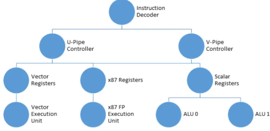
Figure 3.6: Intel Xeon Phi Core Micro-architecture.
The Xeon Phi uses two separate pipelines on each core, the U-pipe and the V-pipe, although the V-pipe can only execute a subset of the U-pipe instructions. However, as both pipes can
nicate with the ALUs, each core is able to execute two separate instructions per clock cycle [23]. The coprocessor’s cores each consist of three separate processing units, the scalar processor, the x87 floating point unit (FPU), and the vector processing unit (VPU), as seen in Figure 3.6. The FPU works as normal in other systems, capable of doing arithmetic on floating point values, however, the scalar unit consists of two separate ALUs in order to complete two operations per clock cycle. The VPU has a separate pipeline, seen in Figure 3.7, once the instruction reaches the write back stage of the core pipeline.
Figure 3.7: Intel Xeon Phi Core Pipeline Stages.
Intel Xeon Phi Vector Processing Unit
Due to the number of arithmetic calculations required for molecular dynamics simulations, the Vector Processor Unit (VPU) of the Xeon Phi becomes extremely important. The VPU receives its data from the L1 cache through a dedicated 512-bit bus, and is capable of communicating to the core to stall as necessary.
The vector processor is a 512-bit Single Instruction Multiple Data (SIMD) unit, capable of working on up to 16 single precision (SP) floating point values, or 8 double precision (DP) floating point values simultaneously. The unit can process one load and an operation in the same cycle, with ternary operands - two source, and one destination. Each VPU consists of 8 UALUs, each containing 2 SP ALUs and one DP ALU.
Once the vector operation instructions reach the write back stage of the main pipeline, the VPU’s pipeline takes over (Figure 3.8). In its first stage, E, the VPU detects any dependencies the current instruction requires, and will stall as necessary. The VC1/VC2 stage then completes shuffle and load conversions. In the V1-V4 stages the 4-cycle multiply/add instructions are executed,
At full capacity, the VPU pipeline has a 1-cycle throughput, with a 4-cycle latency. In essence, the VPU will run at maximum efficiency when four threads are running on each core, to account for the 4-cycle latency.
Figure 3.8: Intel Xeon Phi Vector Pipeline Stages.
The VPU also contains an Extended Math Unit (EMU) for single precision transcendental func-tions, such as exponential and square root functions. These instructions utilize Quadratic Minimax Polynomial approximations, and use lookup tables for fast approximations of the transcendental functions. However, utilizing the EMU has additional penalties for some functions in the latency, thereby decreasing the throughput for these functions to 2 cycles or greater, depending upon the function being used [24], see Table 3.2 for some examples.
Instruction Latency (cycles) Throughput (cycles)
Exp 8 2
Log 4 1
Power 16 4
Sqrt 8 2
Div 8 2
Table 3.2: Intel Xeon Phi Extended Math Unit Latency and Throughput.
Intel Xeon Phi Limitations
While the Intel Xeon Phi coprocessor has the ability to perform many operations per second, it does have limitations due to its design. The design of the Xeon Phi’s instruction decoder is for a two-cycle pipeline unit; hence, if only one thread is being used per core, then only 50% of the core’s peak performance can be achieved. It is therefore beneficial, and required to get the best performance, to use two or more threads on each processor core.
The coprocessor also has a clock frequency of only 1.053 GHz, far lower than most modern processors. This lower frequency means that fewer operations are completed per second; however,
the Many Integrated Cores (MIC) architecture of the Xeon Phi overcomes this limitation by con-taining 60 cores per processor. On a per-thread comparison, modern processors will outperform the Xeon Phi, however, at peak performance the Xeon Phi is capable of reaching 2.1 trillion floating point operations per second, far above that of modern processors [23].
Due to the Xeon Phi being based upon an older Pentium P54c processor, instructions are pro-cessed in order, as opposed to modern processors which use out of order architectures, as well as speculative execution. Compared to modern architectures, the in order execution negatively affects the performance of the Xeon Phi. The Xeon Phi also contains 8 GiB of on-board memory for the operating system in addition to mounting a home directory. This limits the amount of data capable of being stored on the system, thereby limiting the size of the configuration systems that can be utilized.
Comparison with GPUs
A Graphics Processing Unit (GPU) is often used to improve performance of computationally ex-pensive tasks, due to its many-core design being well suited for vectorized instructions. A GPU, however, has a limitation in being used only in an offload fashion - meaning that only some in-structions are processed by the GPU, with the majority of inin-structions still processed on the host processor. While the Xeon Phi is cappable of being run in an offload mode, it is still a general purpose processor, so it does not have this limitation, and can process all instructions required for the program.
GPU programming also requires additional work for programmers in order to make their appli-cation compatible with the GPU. Depending upon the appliappli-cation, this could result in an extensive amount of code being added or re-written to use the application programming interface (API) for the GPU. Further, some of these APIs are proprietary and specific to certain brands of GPUs. The Xeon Phi again has the advantage of not requiring programmers to re-write their code to work for the specialized hardware, and instead only requires informing the compiler to generate the proper machine code for the instruction set.
Conversely, a GPU is advantageous in its specialization and focus towards vectorized instruc-tions. GPUs can have hundreds or thousands of processor cores, each carrying out the same in-struction on different pieces of data, which can have substantial benefits in sections of the code which perform the same operations on multiple pieces of data. Since MD simulations do require the same computations just on different data, GPUs can be applied to MD simulations as well.
For the purposes of this work, however, the Xeon Phi’s general purpose design is better suited, as it allows the use of different parallelization techniques, as opposed to the limited vectorized approach which is used by GPUs.
3.6
Implementation
This section introduces the main components of the simulation code and some of the changes that were made to the existing code base, in order to accommodate the hybrid implementation. Some of these changes include the creation of an outer grid for the task scheduler, modified buffers for transferring data to nodes, and modifications to the force calculations.
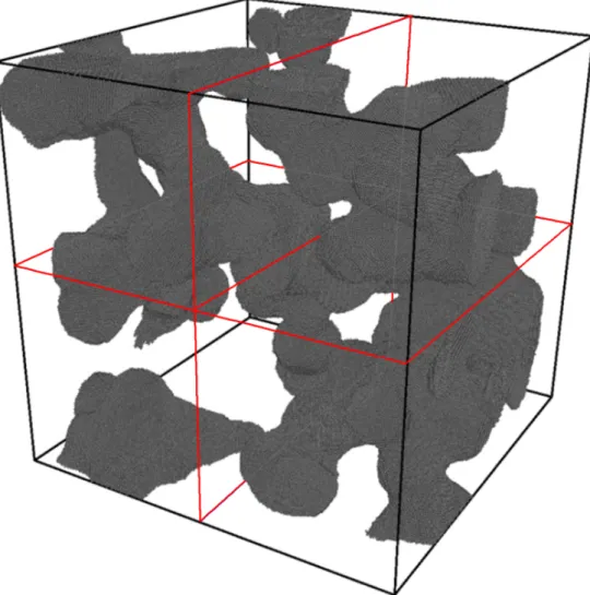
Figure 3.9: Example of the first step of dividing theCu(porous)system using the spatial decom-position method. The lines shown in red show a division of the system in a 2×2 formation.
The proposed hybrid method combines both the spatial decomposition method and the task based method. The simulation system is split into the specified number of domains and the particles are distributed according to the spatial decomposition method, shown in Figure 3.9, after which the
can be scheduled and processed. This allows for each domain to be simulated by its own processor, and from there each processor core can work on separate tasks.
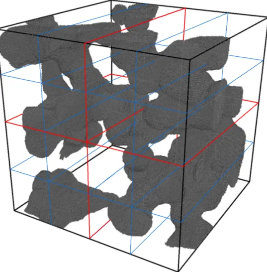
Figure 3.10: Example of the second step of dividing the Cu(porous) system using the cell-task method. The lines shown in red show a division of the system in a 2×2 formation, followed by the blue lines signifying the divisions used by the cell-task method. Note that the cell-task splits the system into significantly more sections than shown.
This overcomes the limitation on the number of cores available that is inherent to the task based method. Further, the dynamic scheduling helps reduce load balancing issues inherent in the spatial decomposition method. This method uses both the Message Passing Interface and the Threading Building Blocks library in order to facility the parallelization. The MPI interface is used for the communication between processes, whereas TBB is used for threading within each process.
3.6.1
The Outer Grid
In the task based implementation, the simulation is split into thousands of smaller cells in a grid pattern. Depending on the simulation configuration settings, these cells are sometimes grouped together to reduce the total number of tasks. The scheduler then dynamically schedules each task in order to calculate the interactions upon each atom within the cells. The scheduler is designed to prevent any two running tasks from accessing the same particle structure, in order to prevent cache coherency issues or thread locking. A rudimentary algorithm as pseudo-code for the inner grid creation for the cell task method can be found in Algorithm 3.1, and the inner and outer grids creation for the hybrid method can be found in Algorithm 3.2.
Algorithm 3.1Pseudo-code of the creation of the inner grid for the cell task parallelism method fori←0toinnerGrid.size()do
innerGrid[i]←null ptr end for
for all particlesdo
dist ←distance f rom center idx←calculateIndex(dist)
innerGrid[idx]appends part end for
A secondary grid, known as the outer grid, is required for this work, which contains only the cells which contain particles which interact with particles in neighbouring domains. Limiting this grid to only relevant particles reduces the need to process each particle within the current domain, which is not necessary for the simulation. This outer grid works alongside the inner grid, which contains all particles located on the current node and is used to schedule the force calculations for all particles interactions occurring within the current sub-domain.
The creation of the outer grid is done when the neighbour-lists are rebuilt. During the construc-tion of the inner grid, which is done using a parallel loop over a range of particles, a thread local copy of the domain data and its surrounding 26 neighbours is created. A thread local copy is used in order to prevent race conditions with the global data, and to prevent the use of thread locking – this prevents degradation of the performance and still allows for the parallel construction of the
grid. This domain data is effectively a linked list of particles which occur on the node. It is split into 27 sections, where particles are sorted based on the neighbouring domains with which they communicate.
This data is filled with information in a step by step process. To begin, the current particle is examined in order to determine if the particle is considered to have passed outside the current domain limits. In this case, the particle has to be transferred to a neighbouring domain. Due to a generally minimal number of particles being transported to other domains, this storage of these particles is done using thread locking; however this does not significantly affect the performance for solid systems.
If the particle is not considered to have moved beyond the bounds of the domain, then the particle’s current location is used in order to determine which of the surrounding 26 neighbouring domains the particle interacts with – this is for the transmission of coordinates and other relevant information to the other domains. Once this has been completed for all particles within the current domain, the thread local data is combined into one larger structure, by consecutively appending the links of each domain data to the next.
At this point, the outer grid is resized and all values within it are set to null pointers. This ensures that previous values, if any, are not accidentally reused when they should not be. The particles which have moved beyond the domain boundary then need to be exchanged with the appropriate domains. Due to the order of particle data being highly important in order to ensure that data is sent to the appropriate neighbouring domains, combined with a generally minimal amount of particles being transferred, this sending of the particles is done in a serial fashion. The particles are removed from the current list of particles in the current domain, then placed into a buffer. Once this has been completed for all particles in the domain requiring transport, the data is then sent to the appropriate neighbouring domains. The receiving of particles, unlike sending, is done in parallel. The particles are appended to the current domain’s list of particles, then added to both the domain structure, and the inner grid. This can be done in parallel due to the incoming particle order not being important.
The domain data can now be finalized in order for appropriate data to be sent to appropriate nodes. A list of communication buffers is added to the buffer list of the domain structures. This is then followed by the creation of a list of particles, which is of equal size to the domain structure’s buffers. This list is kept in the same order which the particles need to be sent to its neighbouring domains, although this does require atomic updates.
In order to send the types and coordinates, the send buffers are first filled with the appropriate data from the particles stored in the previously mentioned list of particles. This is done in order to fill the buffers in parallel in order to reduce the amount of time required preparing the buffers. Once the buffers have been filled, the data can be sent to the surrounding domains. This is done in an attempt to reduce the time required for the communication process.
The next step is to exchange the numbers of particles which are near enough to the borders of the sub-domain to interact with particles in neighbouring domains, which is necessary to allocate the appropriate send and receive buffers for all domains. At the same time, the particle coordinates are also sent to the corresponding domains. Once this is complete, the types (i.e. their chemical elements) of the particles are also exchanged. The types only need to be exchanged when the neighbour-lists are rebuilt, as the types of the particles cannot change, and the order of the particles can only change when the neighbour-lists are rebuilt.
Once the types have been sent, the outer grid can then be constructed. This construction is again done in parallel using threads. The particles are placed into the appropriate grid cell by using the coordinates received from the current domain’s surrounding neighbours. Once the construction of the inner and outer grids is complete the inner scheduler can be created. This inner scheduler is the key component of the cell-task method which is used to schedule tasks in a way such that no two tasks which interact with the same particle are scheduled simultaneously. This is an important aspect, as it is used in the creation of the inner and outer neighbour-lists. The scheduler creation is detailed by Meyer [4].
An outer neighbour-list is needed to keep track of a particle’s neighbours which occur in other spatial domains. This outer neighbour-list is built with the inner grid’s scheduler. At this point, the
Algorithm 3.2Pseudo-code of the creation of the inner and outer grids for the hybrid parallelism method
fori←0toinnerGrid.size()do innerGrid[i]←null ptr end for
for allbu f f ersdo reset bu f f er end for
for alldomainsdo reset domain end for
for all particlesdo
dist ←distance f rom center if particle is out o f domainthen
store to send to proper domain else
dir←associated domain link particle to domain[dir]
idx←calculateIndex(dist)
append particle to innerGrid[idx]
end if end for
fori←0toouterGrid.size()do outerGrid[i]←null ptr end for
ExchangeDeadParticles()
Insert Bu f f ers Into Areas ExchangeParticleNumbers()
ExchangeParticleTypes()
for allReceived particlesdo dist ←distance f rom center idx←calculateIndex(dist)
outerGrid[idx]appends part end for
outer grid scheduler has not been created, however, it is beneficial to continue using the parallel code in order to improve performance.
The particles from all surrounding domains which interact with the particles in the current domain are first loaded into a buffer. Then, for each particle within the domain, an outer neighbour-list is generated using the particles currently in the buffer, if, and only if, the surrounding particle is within the range of the current particle. A counter is used to keep track of the number of particles added to the outer neighbour-list for each particle – if there are none, then the value is set to zero. These particle lists are then appended to the appropriate particle structures, which indicates where their outer neighbour-lists are.
The outer grid is then used to link all particles interacting with other domains. This allows for pointers to the next particle which contains links to particles in other domains to be added to the grid. The location of the particle is used to assign the particle to a specific cell within the grid. The outer scheduler can now be created, using the same methods as the inner scheduler, except it uses the outer grid to only schedule particles which have neighbours in other domains.
The schedulers are required because they ensure that no two tasks are running in parallel which would affect the same particle. Several functions in the simulation code take advantage of Newton’s Third Law of Motion, which requires accessing and modifying the particle being examined and all of its neighbours. By taking advantage of this, the number of calculations is effectively cut in half.
3.6.2
Force Calculations
The calculations of the forces are dependent upon the type of interaction model being used. By following the pattern found in Equation 2.1, the potentials used throughout this work can all follow the same steps. The basic algorithm for many-body potentials can be found in the pseudo-code implementation of the cell task method in Algorithm 3.3 and the hybrid method in Algorithm 3.4. For a many-body potential, such as the Mendelev or Tight-Binding Potentials, the coordinates of the particles near the border of the domain must first be exchanged with neighbouring domains. The function is then executed for all particles within the current domain, which gives information
Algorithm 3.3 Pseudo-code of the force calculations of many-body potentials for the cell task method
for all particlesdo calculateρ
end for
for all particlesdo calculate F and F0 end for
for all particlesdo calculateφ
end for
about how many and how close neighbours are to the current particle, which is summed up into a single value. These calculations are done using the tasks created for the inner grid in order to do the calculations in parallel.
The program will then wait until it receives particle data from its neighbouring domains. This wait is generally kept minimal due to the sending of data prior to the calculations of theρ function.
Once the particle data is received from all neighbours, the calculation ofρ is again done, this time
using the outer scheduler. These values are again added to the single resulting value from the previous calculations.
These results are used to calculate the embedding function F. The derivatives of F are then computed, which givesF0. This is done in parallel over blocks of particles within the entire domain, but does not require the scheduler as they only affect the particle currently being examined, and not their neighbours. Once this is complete, the results are sent to the neighbouring domains for particles which interact with those neighbours. For the Lennard-Jones potential, the above calculations are not necessary. To stick with the model in Equation 2.1, we simply set the result ofF to zero, and the above functions are no longer necessary, other than the initial distribution of particle coordinates.
The next step is to calculate the forces on each particle, which is done in theφ function. The
force calculations use the results from the derivative of the embedding function. This again uses the inner scheduler for task based parallelism. The function further calculates the derivatives of the
Algorithm 3.4 Pseudo-code of the force calculations of many-body potentials for the hybrid method
ExchangeParticleCoordinates()
for all particlesdo
calculateρ o f inner particles
end for
WaitForReceive()
for all particlesdo
calculateρ o f outer particles
end for
for all particlesdo calculate F and F0 end for
for all particlesdo
calculateφ o f inner particles
end for
WaitForReceive()
for all particlesdo
calculateφ o f outer particles
end for
forces, and the pair potential. Once the calculations ofφ are complete, the simulation will again
wait until the results from surrounding domains are received. Once this data has been received, the simulation will continue with the calculation of the forces generated upon the particles within the domain from particles in the neighbouring domains, using the outer scheduler.
The simulation will then combine data from all threads to calculate the total potential energy of each domain, which is then summed over all domains. The results of each of these steps is then utilized to update the positions and velocities of all particles within each of the domains.
3.7
Analysis
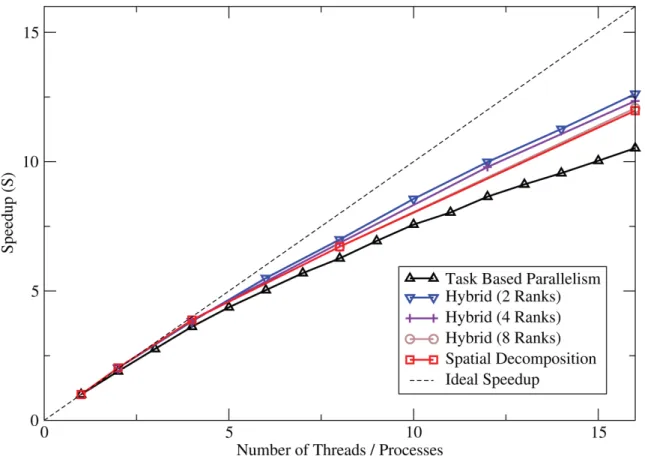
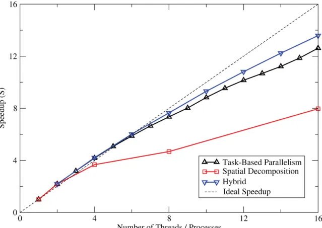
On both hardware systems, a variety of combinations of threads and MPI ranks are used, in order to gauge and compare performance gains. The analysis is based upon the strong scaling speedups, S, as measured against baseline runs using a single MPI rank and a single thread. In addition to the simulations using the hybrid method, all MPI runs were carried out using a single thread per MPI rank, and all threaded runs on the multi-core system using a single MPI rank. The speedup is calculated using Equation 3.1, wheretbaseis the time taken for the baseline run, andtcurrent is the time taken for the current run of the simulation.
S
=
t
baset
current(3.1)
On the multi-core systems tests were done using one, two, four, eight, and sixteen MPI ranks with varying numbers of threads to the total number of cores available per system. On the Xeon Phi coprocessor tests employed one, two, four, eight, sixteen, thirty, sixty, one-hundred twenty, and two-hundred forty MPI ranks with varying numbers of threads. Tests were run using the same configurations on multiple compute nodes. With the multi-core processors, up for 4 compute nodes were used; whereas with the Xeon Phi nodes only one compute node was used with both Xeon Phis within the node, with the exception of the Copper Honey Comb systems which used up to 4 compute nodes, and 8 Xeon Phis.
All tests were run for 1000 time steps, each step being 2 femtoseconds long (10−15 seconds), with the neighbour-lists regenerated every 10 time steps. Each set of tests were run five times, taking the average time of each, in order to more accurately measure the time required to perform the simulation on a given system.
The wall clock time is chosen to measure the time required for the tests to complete, and does not include the time required to read and write configurations files, and instead consists of only the time required to simulate the actual interactions of the particles. This time was chosen for two reasons: firstly, the wall clock time is the perceived time of the user and therefore is the