Minimal unroll factor for code generation of software pipelining

Minimal Unroll Factor for Code Generation of Software Pipelining

Mounira B

, Sid-Ahmed-Ali T

, Frederic B

, David G

, Albert C

June 18, 2012

Abstract

We address the problem of generating compact code from software pipelined loops. Although software pipelin-ing is a powerful technique to extract fine-grain parallelism, it generates lifetime intervals spannpipelin-ing multiple loop iterations. These intervals require periodic register allocation (also called variable expansion), which in turn yields a code generation challenge. We are looking for the minimal unrolling factor enabling the periodic register allocation of software pipelined kernels. This challenge is generally addressed through one of: (1) hardware support in the form of rotating register files, which solve the unrolling problem but are expensive in hardware; (2) register renaming by inserting registermoves, which increase the number of operations in the loop, and may damage the schedule of the software pipeline and reduce throughput; (3) post-pass loop unrolling that does not compromise throughput but often leads to impractical code growth. The latter approach relies on the proof that MAXLIVE registers (maximal number of values simultaneously alive) are sufficient for periodic register allocation [10, 13]. However, the best existing heuristic for controlling this code growth — modulo variable expansion [16] — may not apply the correct amount of loop unrolling to guarantee that MAXLIVE registers are enough, which may result in register spills [10].

This paper presents our research results on the open problem of minimal loop unrolling, allowing a software-only code generation that does not trade the optimality of the initiation interval (II) for the compactness of the generated code. Our novel idea is to use the remaining free registers after periodic register allocation to relax the constraints on register reuse.

The problem of minimal loop unrolling arises either before or after software pipelining, either with a single or with multiple register types (classes). We provide a formal problem definition for each scenario, and we propose and study a dedicated algorithm for each problem.

Our solutions are implemented within an industrial-strength compiler for a VLIW embedded processor from STMicroelectronics, and validated on multiple benchmarks suites.

Keywords: Periodic register allocation, software pipelining, code generation, instruction level parallelism,

embed-ded systems, compilation.

1

Introduction

Most high performance numerical applications exhibit intensive computations in loops. Software Pipelining (SWP) is an important instruction scheduling technique for improving the execution rate of inner loops. It combines multiple iterations of the loop body into a compact pipelined kernel to facilitate the exploitation of instruction level parallelism (ILP) [18, 16, 19]. The number of cycles between two successive iterations of the kernel loop is called theinitiation interval.

When a loop is software pipelined, live ranges of variables may extend beyond a single iteration of the loop. As a result, multiple live ranges of the same variable may be in flight at any program point. One may not use regular register allocation algorithms because these different live range instances would create self-interferences in the interference graph [10, 12, 16]. In compiler construction, when no hardware support is available, kernel loop unrolling avoids introducing unnecessary move and spill operations by duplicating the kernel loop body a sufficient number of times

to remove live range’s self-interference. Computing an adequate unroll factor and allocating registers to the separated live range instances is calledperiodic register allocation.

In this research we are interested in the minimal loop unrolling factor which allows a periodic register allocation for software pipelined loops (without inserting spill or move operations). Having a minimal unroll factor reduces code size, which is an important performance measure for embedded systems because they have a limited memory size. On larger machines, such as desktop, server and supercomputers, total memory size is typically much less limited, but code size is nonetheless important for I-cache performance. In addition to minimal unroll factors, it is necessary that the code generation scheme for periodic register allocation does not generate additional spill; the number of registers required must not exceed MAXLIVE (the number of values simultaneously alive). Spill code can increase the initiation interval and thus reduce performance in the following ways:

1. Adding spill code may increase the length of data dependence chains, which may increase the achievable initia-tion interval.

2. Spill code consumes execution resources which restrains the opportunity for achieving a high degree of instruction-level parallelism.

3. Memory requests consume more power than accessing the same values in registers.

4. Memory operations (except with scratch-pad local memories) have unknown static latencies. Compilers usually assume short latencies for memory operations, despite the fact that the memory access may miss the cache. Without good estimates of the performance of a piece of code, the compiler may be guided to bad optimisation decisions

When the schedule of a pipelined loop is known, there are a number of known methods for computing unroll factors and performing periodic register allocation, but none of them is fully satisfactory:

• Modulo Variable Expansion (MVE) [12, 16] computes a minimal unroll factor but may introduce spill code because it does not provide an upper bound on register usage.

• Hendren’s heuristic [13] computes a sufficient unroll factor to avoid spilling, but with no guarantee in terms of minimal register usage or unrolling degree.

• The meeting graph framework [6] which guarantees that the unroll factor will be sufficient to minimise register usage (reaching MAXLIVE), but not that the unroll factor will itself be minimal.

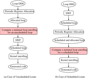
In addition, periodic register allocation can be performed before SWP or after SWP, depending on the compiler construction strategy, as shown in Figure 1. Our article will not debate the best phase order; each compiler has its own characteristic and design implications. Instead we wish to improve the state of the art in loop unrolling minimisation for both possible phase orderings. If periodic register allocation is done before SWP as in Figure 1 (a), the instruction schedule is not fixed, and none of the above periodic register allocation techniques apply.

Contributions. This article advances the state of the art in the following directions:

1. We improve the meeting graph method, achievingsignificantly smaller unroll factorswhilepreserving an opti-mal register usageon already scheduled loops. The key idea of our method is to exploit unused registers beyond the minimal number required for periodic register allocation (MAXLIVE [15])

2. The existing work in the field of kernel unrolling for periodic register allocation deals with already scheduled loops [6, 13, 12, 16]. As mentioned earlier, we also wish to handle not-yet-scheduled loops, on which the cyclic lifetime intervals are not known by the compiler. This article proposes a method for minimal kernel unrolling when SWP has not yet been carried out, bycomputing a minimal unroll factor that is valid for the family of all valid cyclic schedules of the data dependence graph (DDG). On the other hand, if register allocation is performed after SWP as in Figure 1 (b), the instruction schedule is fixed and hence the cyclic lifetime intervals and MAXLIVE are known.

3. We also extend the model of periodic register allocation to handle processor architectures with multiple register types (a.k.a. classes). On such architectures, state-of-the-art algorithms [10, 24] compute thesufficient unrolling degree, i.e., the unrolling degree that should be applied to a loop so that it is always possible to allocate the variables of each register type with a minimal number of registers. This article demonstrates that minimising the unroll factor on each register type separately does not define a global minimal unroll factor, and we provide an appropriate problem definition and an algorithmic solution in this context.

4. We contribute to the enlightenment of a poorly understood dilemma in back-end compiler construction. First, as mentioned earlier and as shown in Figure 1, we offer the compiler designer more choices to control the register pressure and the unroll factor for periodic register allocation at different epochs of the compilation flow. Second, we greatly simplify the phase ordering problem induced by the interplay of modulo scheduling, periodic register allocation, and post-pass unrolling. We achieve this by providing strong guarantees, not only in terms of register usage (the absence of spills induced by insufficient unrolling), but also in terms of reduction of the unroll factor. 5. Our methods are implemented within an industrial-strength compiler for STMicroelectronics’ ST2xx VLIW embedded processor family. Our experiments on multiple benchmarks suites LAO, FFMPEG, MEDIABENCH, SPEC CPU2000, and SPEC CPU2006, are unprecedented in scale. They demonstrate the maturity of the tech-niques and contribute valuable empirical data never published in research papers on software pipelining and pe-riodic register allocation. They also demonstrate the effectiveness of the proposed unroll degree minimisation, both in terms of code size and in terms of initiation intervals (throughput), along with satisfactory compilation times. Better, our techniques outperform the existing compiler for the ST2xx processor family which allocates registers after software pipelining and unrolls using MVE. Our techniques generate less spill code, fewer move operations, and yield a lower initiation interval on average, with a satisfactory code size (loops fitting within the instruction cache). These experiments are also teachful in their more negative results. As expected, they show that achieving strong guarantees on spill-free periodic register allocation yields generally higher unroll factors than heuristics providing no such guarantees like MVE [12, 16]. It was more unexpected (and disappointing) to observe that the initiation intervals achieved with MVE remain generally excellent, despite the presence of spills and a higher number of move operations. This can be explained by the presence of numerous empty slots in the cyclic schedules, where spills and move operations can be inserted, and by the rare occurrence of these spurious operations on the critical path of the dependence graph.

Periodic Register Allocation Scheduled loop

Scheduled and allocated loop

Compute a minimal loop unrolling for a scheduled loop

SWP Loop DDG

Kernel unrolling

Generated code Loop DDG

Periodic Register Allocation

Allocated loop

SWP Scheduled loop

Kernel unrolling

Generated code Compute a minimal loop unrolling

(b) Case of Scheduled Loops (a) Case of Unscheduled Loops

for an unscheduled loop

Outline. The paper is organised as follows. Section 2 describes existing research results that are necessary to under-stand the rest of this article. Section 3 formalises the problem of minimising the loop unrolling degree in the presence of multiple register types when the loop is unscheduled. For clarity, we start the explanation of our loop-unrolling minimisation algorithm in Section 4 with the case of a single register type. Then, Section 5 generalises the solution to multiple register types. When the loop is already scheduled, an adapted algorithm is provided in Section 6 based on the meeting graph framework. Section 7 presents detailed experimental results on standard benchmark suites. In Section 8 we discuss related work on code generation for periodic register allocation, and we explain our contribution compared to the previous work. Finally, we conclude in Section 9.

2

Background

2.1

Loop Model and Software Pipelining

Adata dependence graph(DDG) is a directed multigraph G = (V, E)whereV is a set of vertices representing instructions in a loop (also called statements, nodes, operations) andEis a set of edges representing data dependences (both flow and memory-based).

The modeled processor may have several register types: the set of available registertypesis denoted by_T. For instance,_T =_{BR, GR, F P_}for branch, general purpose, and floating point registers respectively. Register types are sometimes called registerclasses. The number of available registers of typetis noted_Rt_{; it may be less than the}

total number of registers of typetas some architectural registers are often reserved for specific purposes. For a given register typet _{∈ T}, we defineVR,t

⊆V to be the set of statementsu_∈ V that produce values to be stored inside registers of typet. Weut_{denotes the value of typetdefined by an instructionu}

∈ VR,t_{. Indeed, a}

statementumay produce multiple values of distinct types, but we assume a given statement may not produce multiple values of the same type. The value may also be writtenuwhen the type is irrelevant or clear from the context.1

Concerning the set of edgesE, we distinguishflowedges of typet— denotedER,t_{— from the remaining edges.}

A flow edgee= (u, v)of typetrepresents the producer-consumer relationship between the two statementsuandv:u

creates a value read by the statementv. Considering a register of typet, the setE−ER,t_{of non-flow edges are called}

memory-based edges.

Since we focus an loops and take into account loop-carried dependences, the DDG G= (V, E)may be cyclic. Each edgee ∈ E becomes labeled by a pair of values(δ(e), λ(e)). δ : E → Zdefines the latency of edges and

λ : E _→ Zdefines the distance in terms of number of iterations. In order to exploit the parallelism between the instructions belonging to different loop iterations, we rely on periodic scheduling instead of acyclic scheduling, also calledsoftware pipelining(SWP).

SWP can be modeled by a periodic scheduling functionσ:V _→Zand aninitiation intervalII. The operationu of theith_{loop iteration is notedu(i), it is scheduled at dateσ(u) +i}

×II. Here,σ(u)represents the execution (issue) date ofu(0), the clock cycle number ofufor the first loop iteration. The schedule functionσis validif it satisfies the periodic precedence constraints

∀e= (u, v)_∈E:σ(u) +δ(e)_≤σ(v) +λ(e)_×II

SWP allows instructions to be scheduled independently of the original loop iterations barriers. The maximal number of values of typetsimultaneously alive, noted MAXLIVEt, defines the minimal number of registers required to allocate periodically the variables of the loop without introducing spill code. However, since some live ranges of variables span multiple iterations, special care must be taken when allocating registers and colouring an interference graph; this is the core focus of the paper and will be detailed later.

LetRCt_{be the number of registers of typetto be allocated for the kernel of the pipelined loop. If the register}

allocation is optimal, we must have RCt _{= MAXLIVE}t _{for all register typest}

∈ T. We will see that there are only two theoretical frameworks that guarantee this optimality for SWP code generation. Other frameworks have

RCt

≥MAXLIVEt, with no guaranteed upper bound forRCt_.

1_{A few instruction sets allow this, and it can be modeled by node duplication: a node creating multiple results of the same type is split into} multiple nodes of the same type.

2.2

Loop Unrolling after SWP with Modulo Variable Expansion

Code generation for SWP has to deal with many issues: prologue/epilogue codes, early exits from the loops, variables spanning multiple kernel iterations, etc. In our article, we focus on the last point: how can we generate a compact kernel for variables spanning multiples iterations when no hardware support exists in the underlying processor archi-tecture? When no hardware support exists, and when prohibiting the insertion of additional move operations (i.e., no additional live range splitting), kernel loop unrolling is the only option. The resulted loop body itself is bigger but no extra operations are executed in comparison with the original code. Lam designed a general loop unrolling scheme calledmodulo variable expansion(MVE) [16]. In fact, the major criterion of this method is to minimise the loop unrolling degree because the memory size of the i-WARP processor is low [16]. The MVE method defines a minimal unrolling degree to enable code generation after a given periodic register allocation. This unrolling degree is obtained by dividing the length of the longest of all live rangesLTvof variablesvdefined in the pipelined kernel, by

the initiation interval, i.e.,maxvLTv II

.

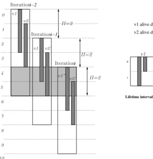
MVE is easy to understand and implement, and it is practically effective in limiting code growth. This is why it has been adopted by several SWP frameworks [5, 15], and included in commercial compilers. The problem with MVE is that it does not guarantee a register allocation with MAXLIVEtregisters of typet, and in general it may lead to unnecessary spills breaking the benefits of software pipelining. A concrete example of this limitation is illustrated in Figures 2 and 3; we will use it as a running example in this section. Figure 2 is a SWP example with two variablesv1

andv2. For simplicity, we consider here a single register typet. New values ofv1andv2are created every iteration.

For instance, the first value ofv1is alive during the time interval[0,2], the other values (v01andv100) are created every

multiple ofII. This figure shows a concrete example with a SWP kernel having two variablesv1 andv2spanning

multiple kernel iterations. In the SWP kernel, we can see that MAXLIVEt= 3.

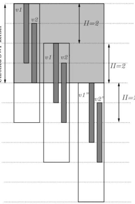
To generate a code for this SWP kernel, MVE unrolls it with a factor of lmax(LTv1,LTv2) II

m

= lmax(3,3)₂ m = 2. Figure 3 illustrates the considered unrolled SWP kernel. The values created inside the SWP kernel arev1,v2,v10, and

v0

2. Because of the periodic nature of the SWP kernel, the variablesv10 andv02are alive as entry and exit values (see the

figure of the lifetime intervals in the SWP kernel). Now, the interference graph of the SWP kernel is drawn, and we can see that it cannot be coloured with less than 4 colours (a maximal clique is_{v1, v2, v01, v20}). Consequently, it is

impossible to generate a code withRCt_{= 3registers, except if we add extra copy operations in parallel. If inserting}

copy operations is not allowed or possible (no free slots, no explicit ILP), then we needRCt_{= 4registers to generate}

a correct code. This example gives a simple case whereRCt_>MAXLIVEt_{, and it is not known ifRC}t_{is bounded.}

As consequence, it is possible that the computed SWP schedule has MAXLIVEt _{≤ R}t, but the code generation performed with MVE requiresRCt_>

Rt_{. This means that spill code has to be inserted even if MAXLIVE}t

≤ Rt_,

which is unfortunate and unsatisfactory.

Fortunately, an algorithm exists that achieves an allocation with a minimal number of registers equal toRCt ₌

MAXLIVEt[6, 10]. This algorithm exploints the meeting graph, introduced in the next section.

2.3

Meeting Graphs (MG)

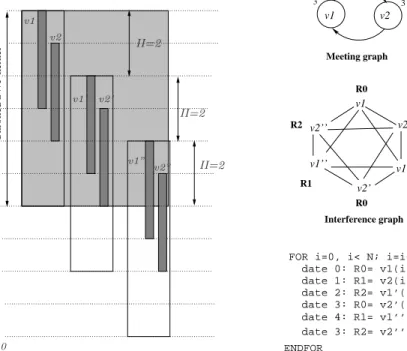
The algorithm of Eisenbeis et al. [6, 10] can generate a periodic register allocation using MAXLIVEtregisters if the kernel is unrolled, thanks to a dedicated graph representation called themeeting graph(MG). It is a more accurate graph than the usual interference graph, as it holds information on the number of clock cycles of each live range and on the succession of the live ranges along the loop iterations. It allows us to compute an unrolling degree which enables an allocation of the loops withRCt_=MAXLIVEt_registers.

Intuitively, the meeting graph is useful because it captures information about pairs of values where one value dies on the same clock cycle that another value becomes alive. If we try to allocate such values to the same register, then there is no dead time when the register contains a dead value. By identifying circuits in the meeting graph, we find sets of live values that can be allocated to one or more registers with no dead time.

Let us consider again the running example in Figure 2. The meeting graph that corresponds to that SWP is illustrated in Figure 4: a node is associated to every variable created in the SWP kernel. Hence we have two nodesv1

andv2. A nodeuis labeled with a weightω(u)corresponding to the length og its respective live range, here 3 clock

0

1

v1 alive during [0,2] v2 alive during [1,3]

Lifetime intervals in the SWP kernel

i i−2 i−1 v1 v2 II=2 II=2 Iteration Iteration Iteration S ta te II=2 10 7 8 9 6 S te a d y 5 4 3 2 1 0 v1’ v2’ v1” v2 v1 v2”

Figure 2: Example to highlight the short-comings of the MVE technique

interval of the first node ends when the sink one starts. By examining the SWP kernel in Figure 2, we see that the copies ofv1end when those ofv2start, and vice-versa. Consequently, in the MG of Figure 4, we have an edge from

v1tov2and vice-versa to model an abstraction of the register reuse for this fixed SWP schedule.

Now, the question is: what is the benefit of such graph structure? Using this graph structure we are able to compute a provably sufficient unrolling factor to apply in order to achieve an optimal register allocation, that isRCt₌

MAXLIVEt[6, 10].

Let us consider the set of the strongly connected components (SCC) of the MG. In our simple example, there is a single SCC. The weight of every SCC numberedkis defined asµk =

P

v∈_SCCkω(v)

II . Note that one of the properties

of the MG is thatP

v∈SCCkω(v)is always a multiple ofII, and P

∀vω(v)

II =MAXLIVE

t_{. In our simple example}

with a single SCC, its weight is equal toµ1= 3+3₂ = 3.

Then, thesufficientunrolling factor computed using the MG is equal toα=lcm(µ1, ..., µk), wherelcmdenotes

the least common multiple [10]. It has been proved that if the SWP kernel is unrolledαtimes, then we can generate code withRCt_=MAXLIVEt_{registers. In the example illustrated in Figure 4, we have a single SCC soα=µ}

1= 3,

which means that the kernel has to be unrolled with a factor equal to 3. The interference graph shows that three colours are sufficient, which allows us to generate correct code with only three registers, rather than the four required with modulo variable expansion (compared to Figure 3).

Without formally proving the correctness of the unrolling factor defined above (the interested reader is invited to study [6, 10]), the intuition behind the least common multiple (LCM) formula comes from the following fact: if we successfully generate code for a SCC by unrolling the kernelµi times, then we can generate a correct code for the

same SCC by unrolling the kernel with any multiple ofµi. Hence, if we are faced with a set of SCCs, it is sufficient to

consider the LCM of theµi’s to have a correct unrolling factor for all the SCCs.

In addition to the previous unroll factor formula, the MG also allows us to guarantee that MAXLIVEtor MAXLIVEt+ 1are sufficient unrolling factors. In the example of Figure 4, we have the coincidence thatα=MAXLIVEt, but this is not always the case. Indeed, one of the purposes of MG is to have unrolling factorsαlower than MAXLIVEt. This objective is not always reachable if we want to haveRCt_=MAXLIVEt_{, Eisenbeis et al. [10] try to reach it by}

decomposing the MG into a maximal number of elementary circuits. In practice, it turns out thatαmay be very high, reducing the practical benefit of register optimalityRCt_=MAXLIVEt_.

The next section recalls a theoretical framework that applies periodic register allocation before SWP, while allow-ing the computation of a sufficient unrollallow-ing degree for a complete set of possible SWP schedules.

v1

v1’ v2’ v2

FOR i=0, i< N; i=i+2

date 0: R0= v1(i) || R1 = R0 date 1: R1= v2(i) || R2 = R1 date 2: R2= v1’(i) || R0=R2 date 3: R0= v2’(i)

ENDFOR

Correct code with 3 registers and parallel copy operations

FOR i=0, i< N; i=i+2 date 1: R1= v2(i) date 2: R2= v1’(i) date 3: R0= v2’(i) ENDFOR

FOR i=0, i< N; i=i+2 date 0: R0= v1(i) date 1: R1= v2(i) date 2: R2= v1’(i) ENDFOR date 3: R3= v2’(i) date 0: R0= v1(i)

Interference graph of the SWP kernel

Impossible correct code with 3 registers

Correct code with 4 registers

Unrolled SWP kernel

0

1

2

3

MVE unrolls the SWP kernel with a factor of 2

Lifetime intervals in the SWP kernel

II=2 II=2 II=2 v1’ v2’ v1” v2 v1 v2” 10 v2 v1 v1’ v2’

Figure 3: SWP kernel unrolled with MVE

2.4

SIRA and Reuse Graphs

Reuse graphsare a generalisation of previously work by de Werra et al. and Hendren et al. [6, 13]. They are used inside a framework called SIRA [23, 24]. Unlike the previous approaches for periodic register allocation, reuse graphs are used before software pipelining to generate a move-free or a spill-free periodic register allocation in the presence of multiple register types. Reuse graphs provide a formalised approach to generating code which requires neither register spills nor move operations. Of course, it is not always possible to avoid spill code, some DDGs are complex enough to always require spilling, the SIRA framework is able to detect such situations before SWP.

A simple way to explain SIRA is to provide an example. All the theory has already been presented in Touati and Eisenbeis [24], and we recently showed that optimising the register requirement for multiple register types in one go is a better approach than optimising for every register type separately [23]. Figure 5(a) provides an initial DDG with two register typest1andt2. Statements producing results of typet1are in dashed circles, and those of typet2are in

bold circles. Statementu1writes two results of distinct types. Flow dependence through registers of typet1are in

dashed edges, and those of typet2are in bold edges.

Each edgeein the DDG is labeled with the pair of values(δ(e), λ(e)). Now, the question is how to compute a periodic register allocation for the loop in Figure 5(a) without hurting the instruction level parallelism if possible.

Periodic register constraints are modeled usingreuse graphs. We associate a reuse graphGreuse,t_{to each register}

FOR i=0, i< N; i=i+3 date 0: R0= v1(i) date 1: R1= v2(i) date 2: R2= v1’(i) date 3: R0= v2’(i) date 4: R1= v1’’(i) date 3: R2= v2’’(i) ENDFOR Unrolled SWP kernel

Correct code with three registers without additional copy operations Interference graph R2 R0 R1 R2 R0 R1 v1 v2 v2’’ v1’’ _v1’ v2’ v1 v2 3 3 Meeting graph II=2 II=2 II=2 10 v1’ v2’ v1” v2 v1 v2”

Figure 4: Example to explain the optimality of the meeting graph technique

(1,0)

(3,2)

(3, 1)

(1,1)

(2,0)

(1,2)

(a) Initial DDG

(b) Reuse Graphs for Register Types t1 and t2

u

u

u

u

_u

_u

Register type

t

u

_u

ν

= 3

ν

= 1

ν

= 3

ν

= 3

ν

= 2

u

Register type

t

Figure 5: Example for SIRA and reuse graphs

SIRA may produce. Note that the reuse graph is not unique, other valid reuse graphs may exist.

A reuse graphGreuse,t _{= (V}R,t_{, E}reuse,t_)containsVR,t_{, i.e., only the nodes writing to registers of typet. These}

nodes are connected byreuse edges. For instance, inGreuse,t2 _{of Figure 5(b), the set of reuse edges isE}reuse,t2 ₌

{(u2, u4),(u4, u2),(u1, u1)}. Also,Ereuse,t1 = {(u1, u3),(u3, u1)}. Each reuse edgeer = (u, v)is labeled by an

integral distanceνt_(e

r), that we callreuse distance. The existence of a reuse edgeer = (u, v)of distanceνt(er)

means thatu(i)(iterationiofu) andu(i+νt_(e

r))(iterationi+νt(er)ofv)share the same destination registerof

typet. Hence, reuse graphs allow to completely define a periodic register allocation for a given loop. In the example of Figure 5(b) and for register typet2, we haveνt2((u2, u4)) = 3andνt2((u4, u2)) = 1.

LetCbe a circuit in the reuse graphGreuse,t_{of typet; we callCareuse circuit. We noteµ}t_{(C) =}P

er∈Cν t_(e

r)

Corollary 1 [24] LetG= (V, E)be a loop DDG with a set of register types_T. Each register typet_{∈ T} is associated with a valid reuse graph Greuse,t _{= (V}R,t_{, E}reuse,t_{). The loop can be allocated with RC}t ₌ P

er∈Ereuse,tν

t_(e r)

registers for each typetif we unroll itαtimes, where:

α=lcm(αt

1,· · ·, α t n)

αti_{is the unrolling degree of the reuse graph of typet}

i, defined as

αt_=lcm(µt_(C

1),· · ·, µt(Cn))

The above corollary seems to be close to the meeting graph result. This is not exactly true, since here we are generalizing the meeting graph result to unscheduled loops in the presence of multiple registers types. Unlike the meeting graph, the above defined unrolling factor is valid for a whole set of SWP schedules, not for a fixed one. In addition, the reuse graph allows us to guarantee that prior to software pipeliningRCt₌P

er∈Ereuse,tν

t_(e

r)≤ Rtfor

any register type, while maintaining instruction level parallelism if possible (by taking care not to increase the critical circuit of the loop, known as theM IIdep).

Note that when compilation time matters, we can avoid unrolling the loop before the SWP step. This avoids increasing the DDG size, which would result in significantly more work for the scheduler. Because we allocate registers directly on the DDG by inserting loop carried anti-dependencies, the DDG can be scheduled without unrolling it. In other words, loop unrolling can be applied at the code generation step (after SWP) in order to apply the register allocation computed before scheduling.

Example 1 Let consider as illustration the example of Figure 5. Hereαt1 =lcm(3,2) = 6andαt2=lcm(3+1,3) =

12. That is, the register typet1requires that we unroll the loop 6 times if we want to consumeRCt1 = 3 + 2 = 5

registers of typet1. At this compilation step, SWP has not been carried out but SIRA guarantees that the computed

unroll factor and register count are valid for any subsequent SWP. As an illustration, a valid sequential trace for the for the register typet1is given in Listing 1 (we do not show the trace for register typet2, and we omit the prologue/epilogue

of the trace).

The reader may check that we have used 5 registers of type t1. According to the reuse graph, every pair of

statements(u1(i), u1(i+ 3))uses exactly the same destination register, because there is a reuse edge(u1, u1)with

a reuse distanceνt1_(u

1, u1) = 3; Every pair of statements(u3(i), u3(i+ 2))uses the same destination register too,

because there is a reuse edge(u3, u3)with a reuse distanceνt1(u3, u3) = 2. We can check in the generated code that

the reuse circuit(u1, u1), which contains a single reuse edge in this example, uses three registers (R1,R2andR3);

The reuse circuit(u3, u3)uses two registers (R4andR5).

Regarding the register typet2, it requires an unrolling factor equal to 12 if we want to consumeRCt2 = 3+1+3 = 7registers of type t2. Consequently, a common valid unroll factor for both the register typest1 andt2is equal to

α=lcm(6,12) = 12. For space reasons, we do not show the full code generation for the loop in Figure 5 with an unrolling factor of 12. However, later in Section 5, we will show how we will minimise the unrolling degree to get a reasonable value equal to 4, it will be then possible to write a reasonably short code for the example.

The main advantage of the meeting graph and reuse graph approaches over MVE is their ability to guarantee spill-free and move-spill-free code generation, before or after SWP. However, they have an important drawback, which is that the unroll factor may be very large. The next section defines the problem of unroll degree minimisation for unscheduled loops. Later, we will extend the problem to scheduled loops.

3

Problem Description of Unroll Factor Minimisation for Unscheduled Loops

The reuse graph method, which guarantees a register allocation with exactly MAXLIVE registers, may result in a large unrolling factor. However, there may be additional unused registers:: each register typetmay have some remaining registersRt₌

Rt

−RCt_(where

Rt_{is the number of available architectural registers of typet). We have developed}

a method to use any remaining registers to reduce the unrolling factor. This method is applied after the periodic register allocation step performed by the SIRA framework. This post-pass minimisation consists in adding zero or more unused registers to each reuse circuit in order to minimise the least common multiple of the size of the circuits (denotedα∗_{). This idea is described in the next problem.}

Listing 1: Example of a sequential kernel code generation for the register typet1 FOR i=0, i<N, i=i+6

u_1(i) : R1 = ... u_2(i) : u_3(i) : R4 = R2... u_4(i) : ...= R4... u_1(i+1): R2 = ... u_2(i+1): u_3(i+1): R5 = R3... u_4(i+1): ...= R5... u_1(i+2): R3 = ... u_2(i+2): u_3(i+2): R4 = R1... u_4(i+2): ...= R4... u_1(i+3): R1 = ... u_2(i+3): u_3(i+3): R5 = R2... u_4(i+4): ...= R5... u_1(i+4): R2 = ... u_2(i+4): u_3(i+4): R4 = R3... u_4(i+4): ...= R4... u_1(i+5): R3 = ... u_2(i+5): u_3(i+5): R5 = R1... u_4(i+5): ...= R5... ENDFOR

Problem 1 (Loop Unroll Minimisation (LUM)) Letαbe the initial loop unrolling degree and let_T =_{t1, . . . , tn}

be the set of register types. For each register typetj ∈ T, letRtj ∈Nbe the number of remaining registers after a periodic register allocation for this register type. Letkj be the number of reuse circuits of typetj. We noteµi,tj ∈N

as the weight of theith_{reuse circuit of the register typet}

j. For each reuse circuitiand each register typetj, we must

compute the added registersri,tj such that we find a new periodic register allocation with a minimal loop unrolling

degree. This is described by the following constraints: 1. α∗ _{= lcm(lcm(µ} 1,t1 +r1,t1, . . . , µk1,t1 +rk1,t1), . . . , lcm(µ1,tn+r1,tn, . . . , µkn,tn+rkn,tn))is minimal (optimality constraint). 2. _∀tj ∈ T, kj X i=1 ri,tj ≤R tj _{(validity constraints)}

That is, this formal problem describes the idea of increasing the number of allocated registers without exceeding the number of available ones (to guarantee the absence of spilling), with the goal of minimising the global unroll factor. Increasing the number of allocated registers is done by increasing the weights of the reuse circuit. If a reuse circuit consists of multiple edges, then increasing the weigth of any edge inside this reuse circuit is a valid solution. This solution is valid as proved in the next lemma. Intuively, this lemma says that if we succeed in building a periodic register allocation withRCt

1registers of typet, then we can build a periodic register allocation withRC2tregisters of

typet, whereRCt

1≤RC2t≤ Rt

Lemma 1 LetG= (V, E)be a loop data dependence graph. LetGreuse,_{be a valid reuse graph of each register type}

t_{∈ T} associated with the loopG. Let_Rbe the number of available registers of typet. Let(ut

i, utj)a single arbitrary

reuse arc inGreuse,t_{with its associated reuse distanceν}t

i,j∈Z. Then: νi,jt ≤ R t =⇒ ∀x∈[0,Rt −νi,jt ], ν t

i,j+xis a valid reuse distance for the reuse arc(u t i, u

t j) Proof:

The proof comes from the formal linear constraints defining the validity ofν variables. These constraints have been defined in [24, 23], that we summarise here. The proof is organised in three subsections. Subsection 3.1 recalls the integer linear program that defines the validity constraints of a reuse graph. Then, Subsections 3.2 and 3.2 prove thatνt

i,j+xdoes not violate these validity conditions.

Our processor model considers both UAL (Unit Assumed Latencies) and NUAL (Non UAL) semantics [21]. Given a register typet_{∈ T}, we model possible delays when reading from or writing into registers of typet. We define two delay functionsδr,t :V 7→Nandδw,t :VR,t7→N.2 These delay functions model NUAL semantics. Thus, the statementureads from a registerδr,t(u)clock cycles after the schedule date

ofu. Also,uwrites into a registerδw,t(u)clock cycles after the schedule date ofu. In UAL, the code

semantics is sequential, these delays are not visible to the compiler, so we haveδw,t=δr,t = 0.

In this proof, we considerG = (V, E)to be a loop DDG, andGreuse,t _{an associated reuse graph to be}

computed using integer linear constraints as defined below.

3.1

Linear Constraints for

ν

Variables

This section briefly recalls the construction of the reuse graph. A recent description for multiple register types can be found in Touati et al. [23, 24]. We say that a value is killed when all its consumers have already read it, and consequently, it does not have to occupy a register anymore. Any last reading instruc-tion is called its killer. If the DDG is already scheduled, then it is easy to compute the killing instrucinstruc-tion and the killing date of each value. However, if the DDG is not already scheduled as in our case, then the killing instruction is not known. For each valuev, we create a virtual killerK, adding edges from all the consumers ofvto the killer nodeK, and we also introduce reuse edges fromKto all subsequent iterations of the consumers ofv.

2_{wis a write to a register of typet, hence the restriction toV}R,t_forδ w,t.

3.1.1 Basic variables

• We define a schedule variable σi ∈ Nfor each statementui ∈ V, includingσKi for each killer Ki. We considerL as a maximal value forσ variables,Lis sufficiently large (for instanceL =

P

e∈Eδ(e)).

Since our instruction scheduling function is a modulo schedule with initiation intervalII, we only consider the integer execution date of the first operation occurrenceσi=σ(ui(0))and the execution

date of any other occurrenceui(k)becomes equal toσ(ui(k)) =σi+k×II.

• A binary variableθt

i,jfor each pair of statements(uti, ujt)∈VR,t×VR,t. It is set to 1 if and only if (ut

i, utj)is a reuse arc;

• A reuse distanceνt

i,j∈Nfor each pair of statements(uti, utj)∈VR,t×VR,tthat is a reuse arc.

3.1.2 Linear constraints

• Data dependences

The schedule must at least satisfy the precedence constraints defined by the DDG.

∀e= (ui, uj)∈E :σj−σi ≥δ(e)−II×λ(e) (1)

• Flow dependences

Each flow dependencee = (ut

i, utj) ∈ER,t,∀t ∈ T means that the statement occurrenceuj(k+

λ(e))reads the data produced byui(k)at timeσj+δr,t(uj) + (λ(e) +k)×II. Then, we must

schedule the killerKiof the statementuiafter allui’s consumers.∀t∈ T,∀ui∈VR,t, ∀uj∈ {v| (ui, v)∈ER,t}|e= (ui, uj)∈ER,t:

σKi ≥σj+δr,t(uj) +II×λ(e) (2)

• Storage dependences

There is a storage dependence between Ki and utj if (uit, utj) is a reuse arc of type t. ∀t ∈

T,_∀(ui, uj)∈VR,t×VR,t:

θi,jt = 1 =⇒σKi−δw,t(uj)≤σj+II×ν t i,j

This involvement can result in the following inequality:_∀t_{∈ T},_∀(ut

i, utj)∈VR,t×VR,t,

σj−σKi+II×ν

t

i,j+M1×(1−θi,jt )≥ −δw,t(uj) (3)

whereM1is an arbitrarily large constant.

If there is no register reuse between two statementsuianduj, thenθi,jt = 0and the storage

depen-dence distanceνt

i,jmust be set to 0 in order to not be accumulated in the objective function.

∀(ui, uj)∈VR,t×VR,t: νi,jt ≤M2×θti,j (4)

whereM2is an arbitrarily large constant.

• Reuse relations

The reuse relation of typetmust be a bijection fromVR,t_toVR,t_{. A register of typetcan be reused}

by one statement and a statement can reuse one released register: ∀ut i ∈V R,t_: X ut j∈VR,t θt i,j= 1 (5) ∀ut j ∈V R,t_: X ut i∈VR,t θt i,j= 1 (6)

From the above integer linear program, we see that theν variables are constrained by Inequality 4 and 3. The two following subsections treat them separately.

3.2

Valid Upper Bounds of

ν

Variables (Inequality 4)

From the above linear constraints, we prove here that increasing the values ofν variables does not violate the upper bounds ofνvariables.

The constraints which define an upper bound forν variables are defined by Inequality 4: ∀(ui, uj)∈VR,t×VR,t: νi,jt ≤M2×θti,j

We have two cases regardingθt

i,j∈ {0,1}value: 1. θt i,j = 0 =⇒ν t i,j≤0. Sinceν t i,j ∈N=⇒ν t

i,j = 0. This means that if(u t i, u

t

j)is not a reuse

arc, then its reuse distance is equal to zero. 2. θt

i,j= 1 =⇒νi,jt ≤M2. SinceM2is arbitrarily large, this means thatνi,jt can arbitrarily verify

this condition. In other words, this means that if(ut

i, utj)is a reuse arc, then its reuse distance

can be arbitrarily large too.

We can decide for a proper finite value forM2that verifies Inequality 4:

By assumptionνt

i,j ≤ Rt=⇒νi,jt ≤maxt∈T Rt. We can deduce a finite value forM2asM2 = maxt∈TRt. The formal result of our lemma is directly deduced from the assumption thatνi,jt ≤ Rt,

and by setting the natural numberx=_Rt

−νt

i,j, we have obviouslyνi,jt +x≤M2.

The next section checks thatνt

i,j+xalso verifies the other linear constraints.

3.3

Storage Constraints on

ν

_{Variables (Inequality 3)}

The other constraints onν variables are those of Inequality 3:

σj−σKi+II×ν

t

i,j+M1×(1−θi,jt )≥ −δw,t(uj) =⇒νi,jt ≥

−σj+σKi−M1×(1−θ t i,j)−δw,t(uj) II Sincex=_Rt −νt i,j≥0 =⇒νi,jt +x≥ −σj+σKi−M1×(1−θti,j)−δw,t(uj II

This means that the valueνt

i,j+xverifies the storage constraints too. Consequently, it constitutes a valid

reuse distance.

y For clarity, we first present a solution to Problem 1 in the case of a single register type.

4

Algorithmic Solution for Unroll Factor Minimisation: Single Register Type

In this section, we solve the problem of minimal unroll degree in the case of a single register type, based on reuse graphs (unscheduled loops). When we consider a single register type, then we have a single reuse graph for the considered register type. The formula for computing the unrolling degree becomes equal to a single LCM of the weights of the reuse circuits of the implicit register type. By replacing the notations ofµi,t (ri,t andRtresp.) byµi

(riandRresp.), Problem 1 amounts to the following one.

Problem 2 (LCM-MIN) LetR _∈Nbe the number of remaining registers. Letµ1, . . . , µk ∈Nbe the weights of the

reuse circuits. Compute the added registersr1, . . . , rk ∈Nsuch that: 1. Pk

i=1ri ≤R(validity constraints)

To our knowledge, Problem 2 has no simple, closed-form solution, and its algorithmic complexity is still an open problem3_.

Before stating our solution for Problem 2, we propose to find a solution for a sub-problem that we call Fixed Loop Unrolling Problem. The solution of this sub-problem constitutes the basis of the solution of Problem 2. The Fixed Loop Unrolling Problemproposes to find, for a fixed unrolling degreeβ, the number of registers that should be added to each circuit to ensure that the size of each circuit is a divisor ofβ. That is, we find the number of registers added to each circuitr1, ..., rksuch thatP

k

i=1ri ≤Randβ is a common multiple of the different updated weights

µ1+r1, ....+µk+rk. A formal description is given in the next section.

4.1

Fixed Loop Unrolling Problem

We formulate theFixed Loop Unrolling Problemas follow:

Problem 3 (Fixed Loop Unrolling Problem) LetR _∈Nbe the number of remaining registers. Letµ1, . . . , µk ∈N

be the weights of the reuse circuits. Given a positive integerβ, compute the different added registersr1, . . . , rk ∈N such that:

1. Pk

i=1ri ≤R

2. βis the common multiple of the news circuits weightsµ1+r1, . . . , µk+rk

To improve readability, we useCMto denote common multiple.

Before describing our solution for Problem 3, we state Lemma 2 and Lemma 3 that we need to use afterwards.

Lemma 2 Let us note some properties of theFixed Loop Unrolling Problem:

1. β _≥maxiµi=⇒ ∃(r1, . . . , rk)∈Nksuch that:CM(µ1+r1, . . . , µk+rk) =β

2. Letr1, . . . , rk be the solution of Problem 3 such thatP k

i=1riis minimal. IfP k

i=1 ri > RthenFixed Loop

Unrolling Problemcannot be solved.

Proof:

• The first issue can be proved by finding an obvious list of added registers

(r1, . . . , rk)∈Nk such that:CM(µ1+r1, . . . , µk+rk) =β

Let us assume thatβ_≥maxiµi. If we put∀i= 1, k: ri=β−µithen

∀i= 1, k: ri≥0andCM(µ1+r1, . . . , µk+rk) =βbecause∀i= 1, k: µi+ri=β

• The second issue can be proved by contradiction.

3_{Indeed, a similar reduced problem exists in cryptography theory: Given two natural numbersa, b, computex≤R}t_∈

Nsuch thatgcd(a, b+x)

is maximal (gcddenotes the greatest common divisor, GCD). This GCD maximisation problem is defined for two integers only, it is equivalent to minimising the LCM of two integers becauselcm(a, b) = a×b

gcd(a,b). The GCD maximisation problem of two integers is known to be equivalent to the integer factorisation problem: the decision problem of integer factorisation has unknown complexity class till now. It is currently solved with approximate methods devoted to very large numbers [14]. Problem 2 is a generalisation of the GCD maximisation problem. The heuristic presented in [14] is not appropriate in our case because: 1) The problem tackled in [14] deals with two integers only, that we cannot generalise to minimise the LCM to multiple integers becauseLCM(x0,· · ·, xk)=6 _gcdx0₍×···×_x0,···x,xkk) fork >2. 2) We deal with multiple small numbers (in practice, R≤128), allowing to design optimal methods efficient in practice instead of heuristics.

Let us assume that we find another solutionr0

1, . . . , rk0 for the problem 3 such that

Pk

i=1r 0 i ≤ R.

However, in the second part of Lemma 2, we find a list of added registerr1, . . . , rksuch thatP k i=1ri is minimal. Consequently, k X i=1 ri≤ k X i=1 r0

i(by assumption, it is minimal) =⇒R < k X i=1 ri≤ k X i=1 r0 i

which constitues a contradiction withPk

i=1r 0 i ≤R.

Thus, if there exists a list of added registers which fulfill the constraints of the problem 3 such that

Pk

i=1riminimal > RthenFixed Loop Unrolling Problemcannot be resolved.

y

Lemma 3 Letβbe a positive integer andDβbe the set of its divisors. Letµ1, . . . , µk∈Nbe the weights of the reuse

circuits. If we find a list of the added registersr1, . . . , rk∈Nfor Problem 3, then we have the following results:

1. β =CM(µ1+r1, . . . , µk+rk)⇒ ∀i= 1, k: β≥µi

2. β =CM(µ1+r1, . . . , µk+rk)⇒ ∀i= 1, k:∃di, ri=di−µiwithdi∈Dβ∧di≥µi.

Proof:

The first issue can be proved as follows:

βis the common multiple (CM) of the news circuits weightsµ1+r1, . . . , µk+rk

⇒ ∀i= 1, k: β_≥µi+ri (7)

From (7) we have:

∀i= 1, k: β _≥µi+ri ⇒ ∀i= 1, k : β−µi≥ri (8)

From (8) we have:

∀i= 1, k: β _≥µibecause∀i= 1, k: ri≥0(eachri∈N) The first issue is proved.

The second issue can be proved by using the definition of the common multiple (CM) of a set of positive integers. Hence, we have:

βis the common multiple (CM) of the news circuits weightsµ1+r1, . . . , µk+rk

⇒ ∀i= 1, k: µi+riis a divisor ofβ (9) From (9) we have: ∀i= 1, k : µi+riis a divisor ofβ ⇒ ∀i= 1, k : _∃di ∈ Dβ|µi+ri=di (10) From (10) we find: ∀i= 1, k: ri≥0 ∃di ∈ Dβ|µi+ri=di ⇒        ∀i= 1, k ∃di ∈ Dβ : ri=di−µi withdi≥µi

The second issue of Lemma 3 is proved.

y After proving Lemma 3 and by using Lemma 2, we describe our solution for theFixed Loop Unrolling Problemin the next section.

{

{

{

d0= 1

r1=d1−µ1 ri=di−µi rk=dk−µk

dk

µ1 d1 µi di µk dm=β

Figure 6: Graphical solution for the fixed loop unrolling problem

4.2

Solution for the Fixed Loop Unrolling Problem

Proposition 1 Letβbe a positive integer andDβbe the set of its divisors. LetRbe the number of remaining registers.

Letµ1, . . . , µk ∈Nbe the weights of the reuse circuits. A minimal list of the added registers (r1, . . . , rk ∈ Nwith

Pk

i=1riis minimal ) can be found by adding to each reuse circuitµi a minimal valuerisuch asri =di−µiwith

di= min{d∈Dβ|d≥µi}. If we denoteCM as common multiple then the two following implications are true:

1. β =CM(µ1+r1, . . . , µk+rk)∧Pk_i=1ri≤R⇒we find a solution for Problem 3;

2. β =CM(µ1+r1, . . . , µk+rk)∧P

k

i=1ri> R⇒Problem 3 has no solution.

Proof:

In Lemma 3, we have proved that:

β=CM(µ1+r1, . . . , µk+rk) =⇒ ∀i= 1, k: ∃di ∈ Dβ|ri=di−µi ∧ di≥µi (11)

From Equation (11) we have:

riis minimal ⇒diis the smallest divisor ofβ ≥ µi (12)

From Equation (12) a list of the added registersr1, . . . , rk withP k

i=1riis minimal can be defined as

follows:

∀i= 1, k: riis minimal =⇒ ∀i= 1, k: ri =di−µi∧di= min{d∈Dβ|d≥µi}

According to Lemma 2, if we find a list of the added registers (the different values of ri) among the

remaining registers such asPk

i=1 riis minimal ≤ Rthen these different values ofrican be a solution

for theFixed Loop Unrolling Problem. Otherwise, ifPk

i=1riis minimal > Rthen we are sure that there

are no solution for Problem 3.

y Figure 6 represents a graphical solution for the Fixed Loop Unrolling Problem. We assume that the different weights and the different divisors ofβare sorted on the same axis in an ascending order.

Algorithm 1 implements our solution for theFixed Loop Unrolling Problem. This algorithm tries to divideRthe remaining registers among the circuits to achieve a fixed common multiple ofkintegers (the different weights of reuse circuitsµi). It checks ifβcan become the new loop unrolling degree. For this purpose, Algorithm 1 uses Algorithm 2

that returns the smallest divisor just after an integer value. Algorithm 1 finds out the list of added registers among the remaining registersRbetween the reuse circuits (the different values ofri ∀i= 1, k), if such list of added registers

exists. It returns also a booleansuccesswhich takes the following values:

success=

true if Pk

i=1ri≤R

false otherwise

The maximal algorithmic complexity of the Fixed Loop Unrolling Problem is then dominated by the while loop: O((_Rt₎2_).

Algorithm 1Fixed loop unrolling problem

Require: k: the number of reuse circuits;µi: the different weights of reuse circuits;Rt

: the number of architectural registers, and β: the loop unrolling degree

Ensure: the different added registersr1, . . . , rkwithPk_i=1riminimalif it exists and a boolean success R =Rt₋P

1≤i≤kµi{the remaining register} sum←0

success←true{defines if we find a valid solution for the different added registers} i←1{represents the number of reuse circuits}

D←DIVISORS(β,Rt

){calculate the sorted list of divisors ofβthat are≤ Rt

includingβ}

whilei≤k∧successdo

di ← DIV NEAR(µi, D){DIV NEAR returns the smallest divisors ofβgreater or equal toµi} ri←di−µi sum←sum+ri ifsum> Rthen success←false else i←i+ 1 end if end while return (r1, . . . , rk),success

Algorithm 2DIV NEAR

Require: µi: the weight of the reuse circuits;D= (d1, . . . , dn): thendivisors ofβsorted by ascending order

Ensure: dithe smallest divisors ofβgreater or equal toµi i←1{represents the index of the divisor ofβ}

whilei≤ndo ifdi ≥ µithen return (di) end if i←i+ 1 end while Algorithm 3DIVISORS

Require: β: the loop unrolling degree;Rt

: the number of architectural registers

Ensure: Dthe list of the divisors ofβthat are≤ Rt

, includingβ bound←min(Rt , β/2) D← {1} ford= 2to bounddo ifβ mod d= 0then

D←D∪ {d} {Keep the list ordered in ascending order}

end if end for

D=D∪ {β}

return (D)

Analysis of the Complexity of Algorithm 1

• Regarding the DIVISORS algorithm:

– The maximal number of iterations is bound_{≤ R}t.

– Inserting an element inside the list costs at mostlog(_Rt_). – The maximal complexity of DIVISORS algorithm isO(Rt

×log(Rt_)).

• Regarding the Fixed Loop Unrolling Problem algorithm:

– Calling DIVISORS costsO(Rt

×log(Rt_)). – The while loop iterates at mostk≤ Rt_times. – At each iteration, calling DIV NEAR costsO(_Rt_).

– The maximal algorithmic complexity of the Fixed Loop Unrolling Problem is then dominated by the while loop:O((_Rt₎2_).

The solution of theFixed Loop Unrolling Problemconstitutes the basis of a solution for theLCM-MIN Problem explained in the next section.

4.3

Solution for LCM-MIN Problem

For the solution of theLCM-MIN Problem(Problem 2) we use the solution of theFixed Loop Unrolling Problemand the result of Lemma 3. According to Lemma 3, the solution spaceS forα∗ _{(the solution ofLCM-MIN Problem) is}

bounded byα, the initial unroll factor.

∀i= 1, k: α∗_≥µ i(From Lemma 3) α∗_≤α ⇒ max 1≤i≤kµi≤α ∗ ≤α

In addition,α∗_{is a multiple of eachµ}

i+riwith0 ≤ ri ≤R. If we assume thatµk = max1≤i≤kµi thenα∗ is a

multiple ofµk+rkwith0≤rk≤R. Furthermore, the solution spaceScan be defined as follows:

S={β ∈N|βis multiple of(µk+rk)∀rk= 0, R ∧ µk≤β≤α}

After describing the setSof all possible values ofα∗_{. The minimalα}∗_{, that is the solution for Problem 2, is defined}

as follows: α∗= min{β ∈S|∃(r1, . . . , rk)∈Nk∧lcm(µ1+r1, . . . , µk+rk) =β∧ k X i=1 ri≤R}

Figure 7 portrays all values of the setSas a partial lattice. An arrow between two nodes means that the value in the first node is less than the value of the second node:a_→b=_⇒a < b. The valueµkrepresents the value of the reuse

circuit numberk. Because we assumed thatµvalues are sorted in ascending order, µk is the highest weight of all

reuse circuits. αis the initial loop unrolling value. Each node is a potential solution (β) which can be considered as the minimal loop unrolling degree. A dashed node can not be a potential candidate because its value is greater thanα.

Letτ =α div µk be the number of the lines of the lattice. Each line describes a set of multiples. For example, the

linejdescribes a set of multiplesSj={β|∃rk,0≤rk≤Rt, β=j×(µk+rk)∧β≤α}

In order to findα∗, the minimal unroll factor, our solution consists in checking if each node ofScan be a solution for theFixed Loop Unrolling Problem: at last we are sure that the minimum of all these values is the minimal loop unrolling degree.

Despite traversing all the nodes ofS, we describe in Figure 7 an efficient way to find the minimalα∗_{. We proceed}

line by line in the figure. In each line, we apply Algorithm 1 to each node until the value of the predicatesuccess

returned by Algorithm 1 istrueor until we arrive at the last line whenβ=α. If the valueβof the nodeiof the linej

verifies the predicate (success=true), then we have two cases:

1. If the value of this node is less than the value of the first node of the next line then we are sure that this value is optimal (α∗_{=β). This is because all the remaining nodes are greater thanβ(by construction of the latticeS).}

2. Else we have found a unroll factor less than the originalα. We note this new valueα0_{and we try once again to}

minimise it until we find the minimal (the first case). The search space shrinks: S0 ₌

{β _∈ N|∀rk = 0..R :

βis multiple of(µk+rk)∧(j+ 1)×µk ≤β≤α0}.

Algorithm 4 implements our solution for theLCM-MIN Problem. This algorithm minimises the loop unrolling degreeαwhich is the least common multiple ofkreuse circuits whose weights areµ1, . . . , µk. Our method is based

on using the remaining registersR. This algorithm computesα∗_{the minimal value of loop unrolling degree and the}

β=α′ µk µk+ 1 µk+ 2 µk+R 2.µk 2.(µk+ 1) 2.(µk+ 2) 2.(µk+R) 3.µk 3.(µk+ 1) 3.(µk+ 2) 3.(µk+R) β=α′ α α τ.µk

Figure 7: How to traverse the latticeS

Listing 2: Example of a sequential kernel code generation for the register typet1 FOR i=0, i<N, i=i+3

u_1(i) : R1 = ... u_2(i) : u_3(i) : R4 = R3... u_4(i) : ...= R4... u_1(i+1): R2 = ... u_2(i+1): u_3(i+1): R5 = R1... u_4(i+1): ...= R5... u_1(i+2): R3 = ... u_2(i+2): u_3(i+2): R6 = R2... u_4(i+2): ...= R6... ENDFOR

Algorithmic Complexity Analysis of Algorithm 4 In the worst case, Algorithm 1 is processed on all the nodes of

the setSin Figure 7. The setShasR_µ×α

k nodes (µk = maxµiandα=lcm(µ1, ..., µk)). We know that1≤µk ≤ R t_.

Consequently, the size of the setS is less or equal toRt

×α. On each node, we process Algorithm 1. Hence, the maximal algorithmic complexity of isO(R×α×(Rt₎2_{) =O(R}

×(Rt₎2

×lcm(µ1, ..., µk)).

Example 2 Let us come back to the example of Figure 5 on page 8, but we focus on the single register typet1, and

we neglect the other register typet2. There are initially two reuse circuits with two costsµ1=νt1(u1, u1) = 3, and

µ2=νt1(u3, u3) = 2. Thus, as shown in Ex. 1, the initial unroll factor is equal tolcm(3,2) = 6. It is easy to see that

if we increment the reuse distanceνt1_(u

3, u3)from 2 to 3, then the cost of the reuse circuit(u3, u3)becomes equal to

3, and hence the unroll factor becomes equal tolcm(3,3) = 3instead of 6. The new number of allocated registers becomes equal toRCt1 _{= 3 + 3instead of 5 initially. A valid kernel code generation with 6 registers of typet}

1and

an unroll factor equal to 3 is given in Listing 2.

Example 3 Let us consider a more complex example with a set of five reuse circuits with the respective weights:

µ1 = 3, µ2 = 4, µ3 = 5, µ4 = 7, µ5 = 8. The initial number of allocated registers is equal toRC = 3 + 4 + 5 + 7 + 8 = 27. The loop unrolling degreeαis their least common multiple (α=lcm(3,4,5,7,8) = 840). Let us assume that we have_Rt = 32architectural registers in the target processor. So hence we haveR = 32−27 = 5

Algorithm 4LCM-MIN algorithm

Require: k: the number of reuse circuits;µi: the weights of the reuse circuits;Rt

: the number of architectural registers;α: the initial loop unrolling degree

Ensure: the minimal loop unrolling degreeα∗and a listr1, . . . , rkof added registers withPk_i=1riminimal R =Rt₋P

1≤i≤kµi{The remaining registers} α∗←µk{minimal value of loop unrollingα∗}

ifα=α∗∨R= 0then ifR= 0then

α∗←α{αnothing can be done, no remaining registers}

end if else

rk←0{number of registers added to the reuse circuitµk} β←µk{value of the first node in the setS}

j←1{line number j in the setS}

τ ←α div µk{total number of lines in the setS} stop←false{stop=trueif the minimal is found} success←false{predicate returned by Algorithm 1}

whileβ≤α∧ ¬stopdo

{Traversing the setSuntil we find the minimal loop unrolling factor}

success ← F ixed U nrolling P roblem(k, µi,Rt, β){Apply for each node the Algorithm 1}

if¬successthen ifrk< Rthen

rk++{we go to the next node on the same line}

else

rk←0{we go to the first node of the next line} j++

end if

β←j×(µk+rk){compute the new value of the potential new unrolling factorβ}

ifβ > α∧j < τthen

{ignore the dashed node}

rk←0{dashed node, we go to the first node of the next line} j++

β←j×µk

end if else

α∗←β{βmay be the minimal loop unrolling degree}

ifα∗≤ (j+ 1) × µkthen

stop←true{we are sure thatα∗is the minimal loop unrolling degree}

else

α←α∗{we find a new value ofαto minimise} τ ←α div µk rk←0 j++ β←j×µk end if end if end while end if

circuits arer1 = 1, r2 = 0, r3 = 3, r4 = 1, r5 = 0. The new reuse circuits’ weights becomeµ1 = 3 + 1 = 4,

µ2= 4 + 0 = 4,µ3= 5 + 3 = 8,µ4= 7 + 1 = 8,µ5+ 0 = 8. The new number of allocated registers become equal

to4 + 4 + 8 + 8 + 8 = 32. The new unroll factor becomes equal toα∗_{=lcm(4,4,8,8,8) = 8, which means that we}

reduced it by aratio= α

α∗ = 105.

5

Unroll Factor Minimisation in the Presence of Multiple Register Types

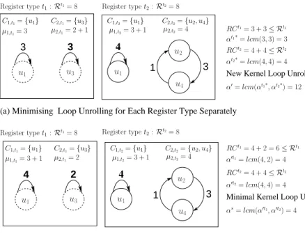
In the presence of multiple register types, minimising the loop unrolling degree of each type separately does not lead to the minimal loop unrolling degree for the whole loop, as illustrated in the following example.

Example 4 Let us return to the example in Figure 5 on page 8. We want to minimise the loop unrolling degree of

the initial reuse graph in Figure 5(b), where two register typest1,t2are considered. The initial kernel loop unrolling

degreeα= 12is the LCM ofαt1 _{= 6andα}t2 _{= 12which are respectively the LCM of the different reuse circuits}

weights for each register type. In this configuration, let us assume that we have_Rtj _{= 8available architectural}

registers in the processor for each register typetj. Hence we haveRt1 = 8−5 = 3(resp Rt2 = 1) remaining

registers for register typet1(respt2). By applying the loop unrolling minimisation for each register type separately

as studied in Section 4, the minimal loop unrolling degree for each register type becomes:αt1∗_{= 3for register type}

t1andαt2

∗

= 4for register typet2, see Figure 8(a). However, the global kernel loop unrolling degree is not minimal

α0_=lcm(αt1∗_{, α}t2∗_{) = 12. The minimal global kernel loop unrolling degree is computed below.}

In Figure 8(b), we provide a solution where the minimal loop unrolling degree isα∗ _{= 4< α}0_{. The unroll factor}

oft1is equal to 4, which is not its minimal value (equal to 3 as shown above). However, the global unroll factor that

satisfies botht1andt2is minimal and equal to 4. The minimal number of registers added to each reuse circuit of each

type are:r1,t1 = 1,r2,t1 = 0,r1,t2 = 1,r2,t2 = 0. Note thatri,tj is the number of registers added to thei th_reuse

circuit of the typetj. Our method explained in the following sections guarantees that the new number of allocated

registers will not exceed the number of architectural registers for each register typetj.

Now let us examine an example of a valid code generation associated to the reuse graphs of Figure 8(b), even though at this stage of compilation, the loop is not yet scheduled. Listing 3 shows a kernel code generation for the register typet1only: registers of typet1 are named with the prefixR. The number of allocated registers isRCt1 = 4 + 2 = 6and the unroll factor is equal to 4. Listing 4 shows a kernel code generation for the register typet2only:

registers of typet2are named with the prefixS. The number of allocated registers isRCt2 = 4 + (1 + 3) = 8and

the unroll factor is equal to 4. The kernel code generation that is correct for botht1andt2is given in Listing 5 and

the unroll factor is minimal and equal to 4: note that the statementu1 has two destination registers of two distinct

types, as previously illustrated in the DDG of Figure 5(a). As can be seen, the initial unroll factor was equal to 12, as computed in Example 1 in page 9, we minimise it here to 4, which is the optimal value. We also guarantee that the number of extra used registers does not exceed the number of remaining registers.

Listing 3: Kernel code generation for register typet1 FOR i=0, i<N, i=i+4

u_1(i): R1 = u_2(i): u_3(i): R5 = R4 +... u_4(i): ...= R5 +... u_1(i+1): R2 = u_2(i+1): u_3(i+1): R6 = R1 +... u_4(i+1):...= R6 +... u_1(i+2): R3 = u_2(i+2): u_3(i+2): R5= R2 + ... u_4(i+2):...= R5 +... u_1(i+3): R4= u_2(i+3): u_3(i+3): R6 = R3 +... u_4(i+4): ...= R6 +... ENDFOR

Listing 4: Kernel code generation for register typet2 FOR i=0, i<N, i=i+4

u_1(i): S1 = S7 +... u_2(i): S5 = S1 +... u_3(i): u_4(i): S6 = S8 + S5 u_1(i+1): S2 = S8 +... u_2(i+1): S6 = S2 +... u_3(i+1): u_4(i+1): S7= S5 + S6 u_1(i+2): S3 = S5 +... u_2(i+2): S7 = S3 +... u_3(i+2): u_4(i+2): S8 = S6 + S7 u_1(i+3): S4 = S6 +... u_2(i+3): S8 = S4 +... u_3(i+3): u_4(i+4): S5 = S7 + S8 ENDFOR

(a) Minimising Loop Unrolling for Each Register Type Separately 4 3 1 3 3 4 3 1 4 2

(b) Minimising Loop Unrolling for all Register Types Conjointly

New Kernel Loop Unrolling:

Minimal Kernel Loop Unrolling:

C2,t1={u3} µ2,t1= 2 + 1 µ1,t1= 3 C1,t2={u1} µ1,t2= 3 + 1 µ2,t2= 4 u2 u4 u1 u3 u1 C2,t2={u2, u4} αt1∗_{=lcm(3,3) = 3} C1,t1={u1} C2,t1={u3} µ2,t1= 2 C1,t2={u1} µ1,t2= 3 + 1 u2 u1 u3 u1 µ2,t2= 4 µ1,t1= 3 + 1 u4 C1,t1={u1}

Register typet1:Rt1= 8 Register typet2:Rt2= 8

α′t2_{=lcm(4,4) = 4} α′t1_{=lcm(4,2) = 4} C2,t2={u2, u4} RC t1_{= 4 + 2 = 6≤ R}t1 αt2∗_{=lcm(4,4) = 4} α′_=lcm(αt1∗_{, α}t2∗_{) = 12} Register typet1:Rt1= 8 Register typet2:Rt2= 8

RCt1_{= 3 + 3≤ R}t1 RCt2_{= 4 + 4≤ R}t2

RCt2_{= 4 + 4≤ R}t2

α∗_=lcm(α′t1_{, α}′t2_{) = 4}

Figure 8: Modifying reuse graphs to minimise loop unrolling factor

Listing 5: Kernel code generation for the two register types conjointly

FOR i=0, i<N, i=i+4 u_1(i): R1,S1 = S7 u_2(i): S5 = S1 u_3(i): R5 = R4 u_4(i): S6 = S8 + S5 + R5 u_1(i+1): R2,S2 = S8 u_2(i+1): S6 = S2 u_3(i+1): R6 = R1 u_4(i+1): S7= S5 + S6 + R6 u_1(i+2): R3,S3 = S5 u_2(i+2): S7 = S3 u_3(i+2): R5 = R4 u_4(i+2): S8 = S6 + S7 + R5 u_1(i+3): R4,S4 = S6 u_2(i+3): S8 = S4 u_3(i+3): R6 = R3 u_4(i+4): S5 = S7 + S8 + R6 ENDFOR

5.1

Search Space for Minimal Kernel Loop Unrolling

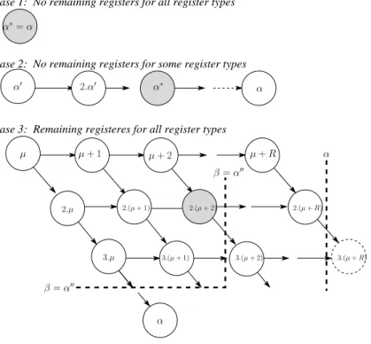
According to the properties of LCM and to the formulation of Problem 1, the search spaceSfor the minimal kernel loop unrollingα∗_{is bounded. In fact, three cases arise:}

Case 1: No remaining registers for all the different register types In this case, the initial loop unrolling degree

cannot be minimisedα∗_=α.

Case 2: No remaining registers for some register types Assume thatαj_{is the loop unrolling degree for the register}

typetj ∈ T. In this way,α=lcm(α1, . . . , αn). We define the subsetT0which contains all the register types such that

there are no remaining registers for these register types after periodic register allocation (_T0 _{⊂ T} such that _T0 =

{t _{∈ T |} Rt _{= 0}

}). If there are no registers left for these register types, we cannot minimise their loop unrolling degrees, see Section 4. Therefore, the minimal global loop unrolling degreeα∗

≥ αj

∀tj ∈ T0. By considering

α0_=lcm

t∈T0(αt), we have the following inequality:

α0 ≤ α∗ ≤ α (13)

In addition, from LCM properties:

α∗ is multiple of α0 (14)

From Equation 13 and Equation 14, the search spaceSis defined as follows:

S={β∈N|βis multiple ofα0 ∧ α0 ≤β≤α} Here, each valueβcan be a potential final loop unrolling degree.

Case 3: All register types have some remaining registers From the associative property of LCM, we have:

α∗=lcm(lcm(µ1,t1+r1,t1, . . . , µk1,t1+rk1,t1), . . . , lcm(µ1,tn+r1,tn, . . . , µkn,tn+rkn,tn))

=⇒α∗=lcm(µ1,t1+r1,t1, . . . , µk1,t1+rk1,t1, . . . , µ1,tn+r1,tn, . . . , µkn,tn+rkn,tn)

The final loop unrolling factorα∗_{is a multiple of each updated reuse circuit weight (µ}

i,tj +ri,tj) with the number of

additional registers (ri,tj) varied from 0 (no added register for this circuit) toR

tj _{(all the remaining registers are added}

to this reuse circuit).

Furthermore, if we assume thatµkn,tn is the maximum weight of all the different circuits for all register types

(µkn,tn= max_t j

(max

i µi,tj)) thenα

∗_{is a multiple of this specific updated circuit (α}∗_{is a multiple of(µ}

kn,tn+rkn,tn)

with0 _≤ rkn,tn ≤ R

tn_{). We notice here that any reuse circuit satisfies this later property, but it is preferable to}

consider the reuse circuit with a maximal weight because it decreases the cardinality of the search spaceS. Finally the search spaceScan be stated as follows:

S={β∈N|βis multiple of(µkn,tn+rkn,tn),∀rkn,tn = 0, R tn _{∧ µ}

kn,tn ≤β ≤α}

After describing the setS of all possible values ofα∗_{(case 2 and case 3), the minimal kernel loop unrollingα}∗ _is

defined as follows:

α∗= min_{β_∈S_|∀tj∈ T,∃(r1,tj, . . . , rkj,tj)∈N

kj _{such that:} βis the Common Multiple (CM) of the following updated reuse circuits weights:

µ1,t1+r1,t1, . . . , µk1,t1+rk1,t1, . . . , µ1,tj +r1,tj, . . . , µkj,tj +rkj,tj, . . . , µ1,tn+r1,tn, . . . , µkn,tn+rkn,tn ∧ kj X i=1 ri,tj ≤R tj_}

Another problem arises here: how to decide if the valueβ can be a potential new loop unrolling? Solving this problem is explained in the next section.