NONLINEAR TIME SERIES ANALYSIS
H O L G E R K A N T Z A N D T H O M A S S C H R E I B E R
p u b l i s h e d b y t h e p r e s s s y n d i c a t e o f t h e u n i v e r s i t y o f c a m b r i d g e The Pitt Building, Trumpington Street, Cambridge, United Kingdom
c a m b r i d g e u n i v e r s i t y p r e s s The Edinburgh Building, Cambridge CB2 2RU, UK 40 West 20th Street, New York, NY 10011–4211, USA 477 Williamstown Road, Port Melbourne, VIC 3207, Australia
Ruiz de Alarc´on 13, 28014 Madrid, Spain Dock House, The Waterfront, Cape Town 8001, South Africa
http://www.cambridge.org C
Holger Kantz and Thomas Schreiber, 2000, 2003 This book is in copyright. Subject to statutory exception and to the provisions of relevant collective licensing agreements,
no reproduction of any part may take place without the written permission of Cambridge University Press.
First published 2000 Second edition published 2003
Printed in the United Kingdom at the University Press, Cambridge Typeface Times 11/14 pt. System LATEX 2ε [tb] A catalogue record for this book is available from the British Library
Library of Congress Cataloguing in Publication data Kantz, Holger, 1960–
Nonlinear time series analysis/Holger Kantz and Thomas Schreiber. – [2nd ed.]. p. cm.
Includes bibliographical references and index. ISBN 0 521 82150 9 – ISBN 0 521 52902 6 (paperback)
1. Time-series analysis. 2. Nonlinear theories. I. Schreiber, Thomas, 1963– II. Title QA280.K355 2003
519.55 – dc21 2003044031 ISBN 0 521 82150 9 hardback ISBN 0 521 52902 6 paperback
The publisher has used its best endeavours to ensure that the URLs for external websites referred to in this book are correct and active at the time of going to press. However, the publisher has no responsibility for the websites
Contents
Preface to the first edition page xi
Preface to the second edition xiii
Acknowledgements xv
I Basic topics 1
1 Introduction: why nonlinear methods? 3
2 Linear tools and general considerations 13
2.1 Stationarity and sampling 13
2.2 Testing for stationarity 15
2.3 Linear correlations and the power spectrum 18
2.3.1 Stationarity and the low-frequency component in the
power spectrum 23
2.4 Linear filters 24
2.5 Linear predictions 27
3 Phase space methods 30
3.1 Determinism: uniqueness in phase space 30
3.2 Delay reconstruction 35
3.3 Finding a good embedding 36
3.3.1 False neighbours 37
3.3.2 The time lag 39
3.4 Visual inspection of data 39
3.5 Poincar´e surface of section 41
3.6 Recurrence plots 43
4 Determinism and predictability 48
4.1 Sources of predictability 48
4.2 Simple nonlinear prediction algorithm 50
4.3 Verification of successful prediction 53
4.4 Cross-prediction errors: probing stationarity 56
4.5 Simple nonlinear noise reduction 58
vi Contents
5 Instability: Lyapunov exponents 65
5.1 Sensitive dependence on initial conditions 65
5.2 Exponential divergence 66
5.3 Measuring the maximal exponent from data 69
6 Self-similarity: dimensions 75
6.1 Attractor geometry and fractals 75
6.2 Correlation dimension 77
6.3 Correlation sum from a time series 78
6.4 Interpretation and pitfalls 82
6.5 Temporal correlations, non-stationarity, and space time
separation plots 87
6.6 Practical considerations 91
6.7 A useful application: determination of the noise level using the
correlation integral 92
6.8 Multi-scale or self-similar signals 95
6.8.1 Scaling laws 96
6.8.2 Detrended fluctuation analysis 100
7 Using nonlinear methods when determinism is weak 105
7.1 Testing for nonlinearity with surrogate data 107
7.1.1 The null hypothesis 109
7.1.2 How to make surrogate data sets 110
7.1.3 Which statistics to use 113
7.1.4 What can go wrong 115
7.1.5 What we have learned 117
7.2 Nonlinear statistics for system discrimination 118
7.3 Extracting qualitative information from a time series 121
8 Selected nonlinear phenomena 126
8.1 Robustness and limit cycles 126
8.2 Coexistence of attractors 128 8.3 Transients 128 8.4 Intermittency 129 8.5 Structural stability 133 8.6 Bifurcations 135 8.7 Quasi-periodicity 139 II Advanced topics 141
9 Advanced embedding methods 143
9.1 Embedding theorems 143
9.1.1 Whitney’s embedding theorem 144
9.1.2 Takens’s delay embedding theorem 146
Contents vii
9.3 Filtered delay embeddings 152
9.3.1 Derivative coordinates 152
9.3.2 Principal component analysis 154
9.4 Fluctuating time intervals 158
9.5 Multichannel measurements 159
9.5.1 Equivalent variables at different positions 160
9.5.2 Variables with different physical meanings 161
9.5.3 Distributed systems 161
9.6 Embedding of interspike intervals 162
9.7 High dimensional chaos and the limitations of the time delay
embedding 165
9.8 Embedding for systems with time delayed feedback 171
10 Chaotic data and noise 174
10.1 Measurement noise and dynamical noise 174
10.2 Effects of noise 175
10.3 Nonlinear noise reduction 178
10.3.1 Noise reduction by gradient descent 179
10.3.2 Local projective noise reduction 180
10.3.3 Implementation of locally projective noise reduction 183
10.3.4 How much noise is taken out? 186
10.3.5 Consistency tests 191
10.4 An application: foetal ECG extraction 193
11 More about invariant quantities 197
11.1 Ergodicity and strange attractors 197
11.2 Lyapunov exponents II 199
11.2.1 The spectrum of Lyapunov exponents and invariant
manifolds 200
11.2.2 Flows versus maps 202
11.2.3 Tangent space method 203
11.2.4 Spurious exponents 205
11.2.5 Almost two dimensional flows 211
11.3 Dimensions II 212
11.3.1 Generalised dimensions, multi-fractals 213
11.3.2 Information dimension from a time series 215
11.4 Entropies 217
11.4.1 Chaos and the flow of information 217
11.4.2 Entropies of a static distribution 218
11.4.3 The Kolmogorov–Sinai entropy 220
11.4.4 The-entropy per unit time 222
viii Contents
11.5 How things are related 229
11.5.1 Pesin’s identity 229
11.5.2 Kaplan–Yorke conjecture 231
12 Modelling and forecasting 234
12.1 Linear stochastic models and filters 236
12.1.1 Linear filters 237
12.1.2 Nonlinear filters 239
12.2 Deterministic dynamics 240
12.3 Local methods in phase space 241
12.3.1 Almost model free methods 241
12.3.2 Local linear fits 242
12.4 Global nonlinear models 244
12.4.1 Polynomials 244
12.4.2 Radial basis functions 245
12.4.3 Neural networks 246
12.4.4 What to do in practice 248
12.5 Improved cost functions 249
12.5.1 Overfitting and model costs 249
12.5.2 The errors-in-variables problem 251
12.5.3 Modelling versus prediction 253
12.6 Model verification 253
12.7 Nonlinear stochastic processes from data 256
12.7.1 Fokker–Planck equations from data 257
12.7.2 Markov chains in embedding space 259
12.7.3 No embedding theorem for Markov chains 260
12.7.4 Predictions for Markov chain data 261
12.7.5 Modelling Markov chain data 262
12.7.6 Choosing embedding parameters for Markov chains 263
12.7.7 Application: prediction of surface wind velocities 264
12.8 Predicting prediction errors 267
12.8.1 Predictability map 267
12.8.2 Individual error prediction 268
12.9 Multi-step predictions versus iterated one-step predictions 271
13 Non-stationary signals 275
13.1 Detecting non-stationarity 276
13.1.1 Making non-stationary data stationary 279
13.2 Over-embedding 280
13.2.1 Deterministic systems with parameter drift 280
13.2.2 Markov chain with parameter drift 281
Contents ix
13.2.4 Application: noise reduction for human voice 286
13.3 Parameter spaces from data 288
14 Coupling and synchronisation of nonlinear systems 292
14.1 Measures for interdependence 292
14.2 Transfer entropy 297
14.3 Synchronisation 299
15 Chaos control 304
15.1 Unstable periodic orbits and their invariant manifolds 306
15.1.1 Locating periodic orbits 306
15.1.2 Stable/unstable manifolds from data 312
15.2 OGY-control and derivates 313
15.3 Variants of OGY-control 316
15.4 Delayed feedback 317
15.5 Tracking 318
15.6 Related aspects 319
A Using the TISEAN programs 321
A.1 Information relevant to most of the routines 322
A.1.1 Efficient neighbour searching 322
A.1.2 Re-occurring command options 325
A.2 Second-order statistics and linear models 326
A.3 Phase space tools 327
A.4 Prediction and modelling 329
A.4.1 Locally constant predictor 329
A.4.2 Locally linear prediction 329
A.4.3 Global nonlinear models 330
A.5 Lyapunov exponents 331
A.6 Dimensions and entropies 331
A.6.1 The correlation sum 331
A.6.2 Information dimension, fixed mass algorithm 332
A.6.3 Entropies 333
A.7 Surrogate data and test statistics 334
A.8 Noise reduction 335
A.9 Finding unstable periodic orbits 336
A.10 Multivariate data 336
B Description of the experimental data sets 338
B.1 Lorenz-like chaos in an NH3laser 338
B.2 Chaos in a periodically modulated NMR laser 340
B.3 Vibrating string 342
B.4 Taylor–Couette flow 342
x Contents
B.6 Heart rate during atrial fibrillation 343
B.7 Human electrocardiogram (ECG) 344
B.8 Phonation data 345
B.9 Postural control data 345
B.10 Autonomous CO2laser with feedback 345
B.11 Nonlinear electric resonance circuit 346
B.12 Frequency doubling solid state laser 348
B.13 Surface wind velocities 349
References 350
Chapter 1
Introduction: why nonlinear methods?
You are probably reading this book because you have an interesting source of data and you suspect it is not a linear one. Either you positively know it is nonlinear because you have some idea of what is going on in the piece of world that you are observing or you are led to suspect that it is because you have tried linear data analysis and you are unsatisfied with its results.1
Linear methods interpret all regular structure in a data set, such as a dominant frequency, through linear correlations (to be defined in Chapter 2 below). This means, in brief, that the intrinsic dynamics of the system are governed by the linear paradigm that small causes lead to small effects. Since linear equations can only lead to exponentially decaying (or growing) or (damped) periodically oscillating solutions, all irregular behaviour of the system has to be attributed to some random external input to the system. Now, chaos theory has taught us that random input is not the only possible source of irregularity in a system’s output: nonlinear, chaotic systems can produce very irregular data with purely deterministic equations of motion in an autonomous way, i.e., without time dependent inputs. Of course, a system which has both, nonlinearity and random input, will most likely produce irregular data as well.
Although we have not yet introduced the tools we need to make quantitative statements, let us look at a few examples of real data sets. They represent very different problems of data analysis where one could profit from reading this book since a treatment with linear methods alone would be inappropriate.
Example 1.1 (NMR laser data). In a laboratory experiment carried out in 1995 by Flepp, Simonet & Brun at the Physics Department of the University of Z¨urich, a Nuclear Magnetic Resonance laser is operated under such conditions that the amplitude of the (radio frequency) laser output varies irregularly over time. From
1 Of course you are also welcome to read this book if you are not working on a particular data set.
4 1. Introduction: why nonlinear methods?
0 20 40 60 80 100
laser output
time
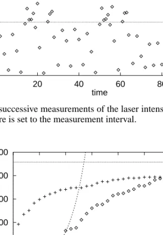
Figure 1.1 100 successive measurements of the laser intensity of an NMR laser.
The time unit here is set to the measurement interval.
0 500 1000 1500 2000 2500 0 5 10 15 20 25 30 35 error prediction time
Figure 1.2 The average prediction error (in units of the data) for a longer sample
of the NMR laser output as a function of the prediction time. For an explanation of the different symbols see the text of Example 1.1.
the set-up of the experiment it is clear that the system is highly nonlinear and random input noise is known to be of very small amplitude compared to the amplitude of the signal. Thus it is not assumed that the irregularity of the signal is just due to input noise. In fact, it has been possible to model the system by a set of differential equations which does not involve any random components at all; see Flepp et al. (1991). Appendix B.2 contains more details about this data set.
Successive values of the signal appear to be very erratic, as can be seen in Fig. 1.1. Nevertheless, as we shall see later, it is possible to make accurate forecasts of future values of the signal using a nonlinear prediction algorithm. Figure 1.2 shows the mean prediction error depending on how far into the future the forecasts are made. Quite intuitively, the further into the future the forecasts are made, the larger
1. Introduction: why nonlinear methods? 5 -4000 3000 -4000 3000 sn sn-1
Figure 1.3 Phase portrait of the NMR laser data in a stroboscopic view. The data
are the same as in Fig. 1.1 but all 38 000 points available are shown.
will the uncertainty be. After about 35 time steps the prediction becomes worse than when just using the mean value as a prediction (horizontal line). On short prediction horizons, the growth of the prediction error can be well approximated by an exponential with an exponent of 0.3, which is indicated as a dashed line. We used the simple prediction method which will be described in Section 4.2. For comparison we also show the result for the best linear predictor that we could fit to the data (crosses). We observe that the predictability due to the linear correlations in the data is much weaker than the one due to the deterministic structure, in particular for short prediction times. The predictability of the signal can be taken as a signature of the deterministic nature of the system. See Section 2.5 for details on the linear prediction method used. The nonlinear structure which leads to the short-term predictability in the data set is not apparent in a representation such as Fig. 1.1. We can, however, make it visible by plotting each data point versus its predecessor, as has been done in Fig. 1.3. Such a plot is called a phase portrait. This representation is a particularly simple application of the time delay embedding, which is a basic tool which will often be used in nonlinear time series analysis. This concept will be formally introduced in Section 3.2. In the present case we just need a data representation which is printable in two dimensions.
Example 1.2 (Human breath rate). One of the data sets used for the Santa Fe Institute time series competition in 1991–92 [Weigend & Gershenfeld (1993)] was provided by A. Goldberger from Beth Israel Hospital in Boston [Rigney et al. (1993); see also Appendix B.5]. Out of several channels we selected a 16 min
6 1. Introduction: why nonlinear methods?
0 5 10 15
air flow
time (min)
Figure 1.4 A time series of about 16 min duration of the air flow through the nose
of a human, measured every 0.5 s.
record of the air flow through the nose of a human subject. A plot of the data segment we used is shown in Fig. 1.4.
In this case only very little is known about the origin of the fluctuations of the breath rate. The only hint that nonlinear behaviour plays a role comes from the data itself: the signal is not compatible with the assumption that it is created by a Gaussian random process with only linear correlations (possibly distorted by a nonlinear measurement function). This we show by creating an artificial data set which has exactly the same linear properties but has no further determinism built in. This data set consists of random numbers which have been rescaled to the distribution of the values of the original (thus also mean and variance are identical) and filtered so that the power spectrum is the same. (How this is done, and further aspects, are discussed in Chapter 4 and Section 7.1.) If the measured data are properly described by a linear process we should not find any significant differences from the artificial ones.
Let us again use a time delay embedding to view and compare the original and the artificial time series. We simply plot each time series value against the value taken a
delay timeτearlier. We find that the resulting two phase portraits look qualitatively
different. Part of the structure present in the original data (Fig. 1.5, left hand panel) is not reproduced by the artificial series (Fig. 1.5, right hand panel). Since both series have the same linear properties, the difference is most likely due to nonlinearity in the system. Most significantly, the original data set is statistically asymmetric under time reversal, which is reflected in the fact that Fig. 1.5, left hand panel, is non-symmetric under reflection with respect to the diagonal. This observation makes it very unlikely that the data represent a noisy harmonic oscillation. Example 1.3 (Vibrating string data). Nick Tufillaro and Timothy Molteno at the Physics Department, University of Otago, Dunedin, New Zealand, provided a couple of time series (see Appendix B.3) from a vibrating string in a magnetic field.
1. Introduction: why nonlinear methods? 7
s(t)
s(t-0.5 sec)
s(t)
s(t-0.5 sec)
Figure 1.5 Phase portraits of the data shown in Fig. 1.4 (left) and of an artificial
data set consisting of random numbers with the same linear statistical properties (right).
y(t)
x(t)
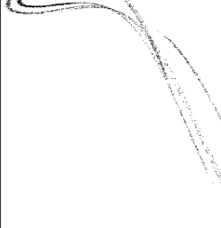
Figure 1.6 Envelope of the elongation of a vibrating string. Line: the first 1000
measurements. Dots: the following 4000 measurements.
The envelope of the elongation of the wire undergoes oscillations which may be chaotic, depending on the parameters chosen. One of these data sets is dominated by a period-five cycle, which means that after every fifth oscillation the recording (approximately) retraces itself. In Fig. 1.6 we plot the simultaneously recorded x-and y-elongations. We draw a solid line through the first 1000 measurements x-and place a dot at each of the next 4000. We see that the period-five cycle does not remain perfect during the measurement interval. This becomes more evident by plotting one point every cycle versus the cycle count. (These points are obtained in a systematic way called the Poincar´e section; see Section 3.5.) We see in Fig. 1.7 that the period-five cycle is interrupted occasionally. A natural explanation could be that there are perhaps external influences on the equipment which cause the system to leave the periodic state. However, a much more appropriate explanation
8 1. Introduction: why nonlinear methods?
0 100 200 300 400 500 600
cycle number
Figure 1.7 Data of Fig. 1.6 represented by one point per cycle. The period-five
cycle is interrupted irregularly.
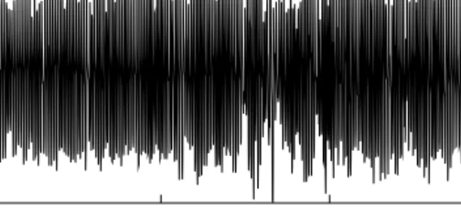
0 5 10 15 20 0 5 0 5 sec [ µ V]
Figure 1.8 Upper trace: electrocardiographic recording of a pregnant woman. The
foetal heart causes the small spikes. Lower trace: the foetal electrocardiogram has been extracted by a nonlinear projection technique.
of the data set is given in Example 8.3 in Section 8.4. The irregular episodes are in fact due to intermittency, a typical phenomenon found in nonlinear dynamical
systems.
Example 1.4 (Foetal electrocardiogram). Let us consider the signal processing problem of extracting the tiny foetal electrocardiogram component from the (small) electrical potentials on the abdomen of a pregnant woman (upper trace in Fig. 1.8). The faster and smaller foetal signal cannot be distinguished by classical linear techniques because both the maternal and foetal electrocardiograms have broad band power spectra. However, using a nonlinear phase space projection technique that was originally developed for noise reduction in chaotic data (Section 10.3.2), it is possible to perform the separation in an automated way. The lower trace in Fig. 1.8 shows the extracted foetal component. More explanations are given in
1. Introduction: why nonlinear methods? 9
Section 10.4. Note that we do not need to assume (nor do we actually expect) that the heart is a deterministic chaotic system.
There is a broad range of questions that we have to address when talking about nonlinear time series analysis. How can we get the most precise and meaningful results for a clean and clearly deterministic data set like the one in the first example? What modifications are necessary if the case is less clear? What can still be done if, as in the breath rate example, all we have are some hints that the data are not properly described by a linear model with Gaussian inputs? Depending on the data sets and the analysis task we have in mind, we will choose different approaches. However, there are a number of general ideas that one should be acquainted with no matter what one’s data look like. The most important concepts analysing complex data will be presented in Part One of the book. Issues which are either theoretically more advanced, require higher-quality data, or are of less general interest will be found in Part Two.
Obviously, in such a diverse field as nonlinear time series analysis, any selection of topics for a single volume must be incomplete. It would be naive to claim that all the choices we have made are exclusively based on objective criteria. There is a strong bias towards methods that we have found either conceptually interesting or useful in practical work, or both. Which methods are most useful depends on the type of data to be analysed and thus part of our bias has been determined by our contacts with experimental groups. Finally, we are no exception to the rule that people prefer the methods that they have been involved in developing.
While we believe that some approaches presented in the literature are indeed useless for scientific work (such as determining Lyapunov exponents from as few as 16 data points), we want to stress that other methods we mention only briefly or not at all, may very well be useful for a given time series problem. Below we list some major omissions (apart from those neglected as a result of our ignorance). Nonlinear generalisations of ARMA models and other methods popular among statisticians are presented in Tong (1990). Generalising the usual two-point autocorrelation function leads to the bispectrum. This and related time series models are discussed in Subba Rao & Gabr (1984). Within the theory of dynamical systems, the analysis of unstable periodic orbits plays a prominent role. On the one hand, periodic orbits are important for the study of the topology of an attractor. Very interesting results on the template structure, winding numbers, etc., have been obtained, but the approach is limited to those attractors of dimension two or more which can be embedded in three dimensional phase space. (One dimensional manifolds, e.g. trajectories of dynamical systems, do not form knots in more than three dimensional space.) We refer the interested reader to Tufillaro et al. (1992). On the other hand, periodic orbit expansions constitute a powerful way of computing characteristic quantities which
10 1. Introduction: why nonlinear methods?
are defined as averages over the natural measure, such as dimensions, entropies, and Lyapunov exponents. In the case where a system is hyperbolic, i.e., expanding and contracting directions are nowhere tangent to each other, exponentially converging expressions for such quantities can be derived. However, when hyperbolicity is lacking (the generic case), very large numbers of periodic orbits are necessary for the cycle expansions. So far it has not been demonstrated that this kind of analysis is feasible based on experimental time series data. The theory is explained in Artuso et al. (1990), and in “The Webbook” [Cvitanovi´c et al. (2001)].
After a brief review of the basic concepts of linear time series analysis in Chap-ter 2, the most fundamental ideas of the nonlinear dynamics approach will be intro-duced in the chapters on phase space (Chapter 3) and on predictability (Chapter 4). These two chapters are essential for the understanding of the remaining text; in fact, the concept of a phase space representation rather than a time or frequency do-main approach is the hallmark of nonlinear dynamical time series analysis. Another fundamental concept of nonlinear dynamics is the sensitivity of chaotic systems to changes in the initial conditions, which is discussed in the chapter about dy-namical instability and the Lyapunov exponent (Chapter 5). In order to be bounded and unstable at the same time, a trajectory of a dissipative dynamical system has to live on a set with unusual geometric properties. How these are studied from a time series is discussed in the chapter on attractor geometry and fractal dimensions (Chapter 6). Each of the latter two chapters contains the basics about their topic, while additional material will be provided later in Chapter 11. We will relax the re-quirement of determinism in Chapter 7 (and later in Chapter 12). We propose rather general methods to inspect and study complex data, including visual and symbolic approaches. Furthermore, we will establish statistical methods to characterise data that lack strong evidence of determinism such as scaling or self-similarity. We will put our considerations into the broader context of the theory of nonlinear dynamical systems in Chapter 8.
The second part of the book will contain advanced material which may be worth studying when one of the more basic algorithms has been successfully applied; obviously there is no point in estimating the whole spectrum of Lyapunov exponents when the largest one has not been determined reliably. As a general rule, refer to Part One to get first results. Then consult Part Two for optimal results. This rule applies to embeddings, Chapter 9, noise treatment, Chapter 10, as well as modelling and prediction, Chapter 12. Here, methods to deal with nonlinear processes with stochastic driving have been included. An advanced mathematical level is necessary for the study of invariant quantities such as Lyapunov spectra and generalised dimensions, Chapter 11. Recent advancements in the treatment of non-stationary signals are presented in Chapter 13. There will also be a brief account of chaotic synchronisation, Chapter 14.
Further reading 11
Chaos control is a huge field in itself, but since it is closely related to time series analysis it will be discussed to conclude the text in Chapter 15.
Throughout the text we will make reference to the specific implementations of the methods discussed which are included in the TISEAN software package.2 Background information about the implementation and suggestions for the use of the programs will be given in Appendix A. The TISEAN package contains a large number of routines, some of which are implementations of standard techniques or included for convenience (spectral analysis, random numbers, etc.) and will not be further discussed here. Rather, we will focus on those routines which implement essential ideas of nonlinear time series analysis. For further information, please refer to the documentation distributed with the software.
Nonlinear time series analysis is not as well established and is far less well un-derstood than its linear counterpart. Although we will make every effort to explain the perspectives and limitations of the methods we will introduce, it will be neces-sary for you to familiarise yourself with the algorithms with the help of artificial data where the correct results are known. While we have almost exclusively used experimental data in the examples to illustrate the concepts discussed in the text, we will introduce a number of numerical models in the exercises. We urge the reader to solve some of the problems and to use the artificial data before actually analysing measured time series. It is a bad idea to apply unfamiliar algorithms to data with unknown properties; better to practise on some data with appropriate known prop-erties, such as the number of data points and sampling rate, number of degrees of freedom, amount and nature of the noise, etc. To give a choice of popular models we introduce the logistic map (Exercise 2.2), the H´enon map (Exercise 3.1), the Ikeda map (Exercise 6.3), a three dimensional map by Baier and Klein (Exercise 5.1), the Lorenz equations (Exercise 3.2) and the Mackey–Glass delay differential equation (Exercise 7.2). Various noise models can be considered for comparison, including moving average (Exercise 2.1) and Brownian motion models (Exercise 5.3). These are only the references to the exercises where the models are introduced. Use the index to find further material.
Further reading
Obviously, someone who wants to profit from time series methods based on chaos theory will improve his/her understanding of the results by learning more about chaos theory. There is a nice little book about chance and chaos by Ruelle (1991). A readable introduction without much mathematical burden is the book by Kaplan & Glass (1995). Other textbooks on the topic include Berg´e et al. (1986), Schuster
12 1. Introduction: why nonlinear methods?
(1988), and Ott (1993). A very nice presentation is that by Alligood et al. (1997). More advanced material is contained in Eckmann & Ruelle (1985) and in Katok & Hasselblatt (1996). Many articles relevant for the practical aspects of chaos are reproduced in Ott et al. (1994), augmented by a general introduction. Theoretical aspects of chaotic dynamics relevant for time series analysis are discussed in Ruelle (1989).
There are several books that cover chaotic time series analysis, each one with different emphasis. Abarbanel (1996) discusses aspects of time series analysis with methods from chaos theory, with a certain emphasis on the work of his group on false neighbours techniques. The small volume by Diks (1999) focuses on a number of particular aspects, including the effect of noise on chaotic data, which are discussed quite thoroughly. There are some monographs which are connected to specific ex-perimental situations but contain material of more general interest: Pawelzik (1991), Buzug (1994) (both in German), Tufillaro et al. (1992) and Galka (2000). Many interesting articles about nonlinear methods of time series analysis can be found in the following conference proceedings volumes: Mayer-Kress (1986), Casdagli & Eubank (1992), Drazin & King (1992), and Gershenfeld & Weigend (1993). Inter-esting articles about nonlinear dynamics and physiology in particular are contained in B´elair et al. (1995). Review articles relevant to the field but taking slightly differ-ent points of view are Grassberger et al. (1991), Casdagli et al. (1991), Abarbanel et al. (1993), Gershenfeld & Weigend (1993), and Schreiber (1999). The TISEAN software package is accompanied by an article by Hegger et al. (1999), which can also be used as an overview of time series methods.
For a statistician’s view of nonlinear time series analysis, see the books by Priestley (1988) or by Tong (1990). There have been a number of workshops that brought statisticians and dynamical systems people together. Relevant proceedings volumes include Tong (1993), Tong (1995) and Mees (2000).