UC Santa Barbara
UC Santa Barbara Electronic Theses and Dissertations
Title
Algorithms and Software for High-Performance Fracture Simulation on GPU Architectures Permalink
https://escholarship.org/uc/item/0br2k5cc Author
Lim, Rone Kwei Publication Date 2017
University of California
Santa Barbara
Algorithms and Software for High-Performance Fracture Simulation
on GPU Architectures
A dissertation submitted in partial satisfaction of the requirements for the
degree of
Doctor of Philosophy
in
Computer Science
by
Rone Kwei Lim
Committee:
Professor Linda R. Petzold, Chair Professor Matthew R. Begley Professor John R. Gilbert
The dissertation of Rone Kwei Lim is approved:
Professor Matthew R. Begley
Professor John R. Gilbert
Professor Linda R. Petzold, Committee Chair June 2017
Algorithms and Software for High-Performance Fracture Simulation on GPU Architectures Copyright © 2017
by Rone Kwei Lim
Acknowledgements
I would like to thank my Ph.D advisor, Professor Linda Petzold, for her mentorship and guidance. I would also like to thank my co-advisor, Professor Matthew Begley, for his support and guidance. I also thank my dissertation committee, Professor John Gilbert, for his support and insight.
I extend a thank you to my collaborator, Will Pro, without whom this dissertation would not have been possible. I would also like to thank my other collaborators, Marcel Utz and Cetin Kaya Koc.
I would like to thank my friends, family members, mentors, teachers, and others who have helped supported me over the years, and the current and former members of Professor Petzold’s research group, as well as members of Professor Begley’s research group.
I gratefully acknowledge financial support from the National Science Foundation through a Graduate Research Fellowship, a Doctoral Scholar Fellowship from UCSB, and the Department of Computer Science at UCSB. Additional support was provided by NSF, DOE, and the UCSB Institute for Collaborative Biotechnologies.
Curriculum Vitae
Rone Kwei Lim
Education
2017 Doctor of Philosophy in Computer Science, University of California, Santa Barbara (expected)
Emphasis: Computational Science and Engineering
2012 Master of Science in Computer Science, University of California, Santa Barbara
2008 Bachelor of Science in Computer Science, California State University, Los Angeles
2008 Bachelor of Science in Applied Mathematics, California State University, Los Angeles
Publications
Lim RK, Petzold LR, Koc CK. Bitsliced high-performance AES-ECB on GPUs. The New Codebreakers 2016, 9100:125-133.
Pro JW, Lim RK, Petzold LR, et al. The impact of stochastic microstructures on the
macroscopic fracture properties of brick and mortar composites. Extreme Mechanics Letters
2015, 5: 1-9.
Lim RK, Pro JW, Begley MR, et al. High-performance simulation of fracture in idealized ‘brick and mortar’ composites using adaptive Monte Carlo minimization on the GPU. The International Journal of High Performance Computing Applications 2016, 30: 186-199. Pro JW, Lim RK, Petzold LR, et al. GPU-based simulations of fracture in idealized brick and mortar composites. Journal of the Mechanics and Physics of Solids 2015, 80: 68-85.
Sanft KR, Wu S, Roh M, et al. StochKit2: software for discrete stochastic simulations of biochemical system with events. Bioinformatics 2011, 27: 2457-2458.
Abstract
Algorithms and Software for High-Performance Fracture Simulation on GPU Architectures
Rone Kwei Lim
Computer simulation of fracture in materials with nonlinear mechanical response can be computationally expensive. These simulations often require a large number of degrees of freedom, and the nonlinearity in the problem can pose difficulties when computing solutions. This work focuses on two material models. The first model consists of rigid bricks
interacting through nonlinear cohesive springs. Fracture in the material occurs through the rupture of the cohesive springs. The second, more complicated, model consists of deformable elements interacting through nonlinear cohesive springs.
In the first model, we assume the bricks are under a quasi-static loading scenario. With this assumption, the problem can be solved using a global Monte Carlo minimization algorithm to minimize the energy of the system. The energy in the system comes from the deformation and rupture of the nonlinear cohesive springs. Since these simulations have a high computational cost, we have developed a GPU-based (Graphics Processing Unit) Monte Carlo minimization algorithm that offers a significant speedup compared to a conventional multithreaded CPU-based algorithm.
With the second model, we have dynamic simulations with explicit time discretization. In this case we compute the force, acceleration, velocity, and position
explicitly. The force in the system comes from both the deformation of the elements as well as the deformation of the nonlinear cohesive springs. We have developed explicit,
CPU-based methods and implicit-explict methods on both CPUs and GPUs. Our implicit-explict GPU-based method achieves substantial performance improvement compared to the explicit, CPU-based method.
We present our GPU-based implementation of AES (Advanced Encryption Standard), which is used in the Monte Carlo minimization algorithm to generate random numbers. Our implementation is substantially faster than CPU-based implementation of AES. It is also faster than previous GPU implementations of AES.
Table of Contents Acknowledgements...iv Curriculum Vitae...v Abstract...vi List of Figures...ix Chapter 1 Introduction...1
Chapter 2 High-performance simulation of fracture in idealized “brick and mortar” composites using adaptive Monte Carlo minimization on the GPU...4
2.1 Background...6
2.1.1 Model...6
2.1.2 Basic Numerical Method...9
2.2 Adaptive Numerical Methods...11
2.3 GPU Architecture...16
2.4 GPU Implementation...21
2.5 Results...25
2.5.1 Performance improvement due to adaptive methods...32
2.6 Conclusion...33
Chapter 3 Bitsliced High-Performance AES-ECB on GPUs...35
3.1 Comparing GPUs...35
3.2 AES Encryption on CPU and GPUs...36
3.3 AES-ECB on the GPUs...37
3.3.1 Bit Ordering...37
3.3.2 Load and Store...38
3.3.3 SubBytes...38
3.3.4 ShiftRows...39
3.3.5 MixColumns...40
3.3.6 AddRoundKey...41
3.3.7 Resistance to Timing-Attack...41
3.4 Results and Conclusion...41
Chapter 4 Integrating material structure with implicit/explicit methods to achieve high performance fracture simulations on GPUs...43
4.1 Material Description...46
4.2 Algorithms...48
4.2.1 Unbolted explicit method...48
4.2.2 Bolted explicit method...50
4.2.3 Bolted implicit-explicit method...52
4.3 GPU Acceleration...53
4.4 Results...55
4.5 Conclusion...64
Chapter 5 Conclusion...65
List of Figures
Figure 1.1. An example simulation output. The colors represent vertical brick stress...2
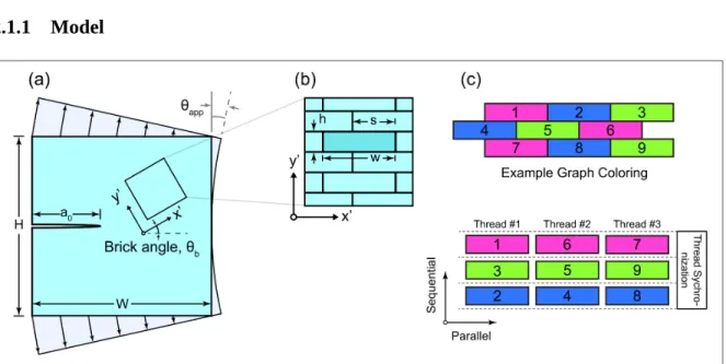
Figure 2.1. (a) Schematic of macroscopic specimen and loading scenario (bending). There is a pre-existing crack in the middle of the specimen. (b) An example configuration of bricks. Many more bricks are used in the actual simulations. (c) Assignment of bricks to threads using graph-coloring. Adjacent bricks are assigned different colors. Bricks of the same color are processed in parallel...6
Figure 2.2. (a) Graph of traction-separation function. (b) Graph of the energy potential, defined as the integral of the traction-separation function...9
Figure 2.3. (a) Adaptive cycle illustration. The old sliding window is labeled windowold, while the new sliding window at the next cycle is labeled windownew. The blue circle is the new energy value, and the red circle is the old energy value. The variance and correlation coefficient are calculated each time the sliding window is updated. (b) Graph of position predictor multiplier. The predictor uses linear prediction when the energy is low, and a combination of linear and constant prediction as the energy increases...12
Figure 2.4. CPU and GPU architectures. A GPU has more transistors devoted to execution, while a CPU has more transistors for cache and control mechanisms...18
Figure 2.5. (a) Peak GFlops of CPUs and GPUs. The peak GFlops is significantly higher on a GPU. (b) Peak memory bandwidth of CPUs and GPUs. The peak bandwidth is significantly higher on a GPU (c) Peak double precision GFLOP/s on the test systems: Nvidia GTX 480 GPU/Core 2 Quad Q6600 CPU and Nvidia GTX 580 GPU/Core i7 2600 CPU...19
Figure 2.6. Flowchart of the overall simulation algorithm...21
Figure 2.7. Diagram of the data structures used in the simulation. Initially, the data structures are in an array of structure format during input processing. It is then rearranged into a structure of array format. Additionally, the individual elements are rearranged according to the graph coloring order...25
Figure 2.8. Simulation output. (a) The colors represent the energy of the bricks. (b) The total energy for various brick orientations...27
Figure 2.9. (a) Initialization time. (b) GPU and CPU simulation times (semilog)...28
Figure 2.10. (a) GPU simulation times with different tolerance values. (b) Final energy value with different tolerance values...29
Figure 2.11. CPU simulation time with different numbers of cores...30
Figure 2.12. Percentage of simulation time for different parts of the algorithm on GTX 480 and 580...31
Figure 2.13. (a) Comparison of GPU simulation time for adaptive vs. non-adaptive algorithms. (b) Relative speedup from using GPU and adaptive methods. The time for Core 2 Quad Q6600 non-adaptive is an estimated runtime based on the difference between GTX 480 adaptive and GTX 480 non-adaptive, and the difference between GTX 480 adaptive and Core 2 Quad Q6600 adaptive, since it takes an impractical amount of time to run the Core 2 non-adaptive case...32
Figure 3.1: The state of one block...38
Figure 3.2: The bitsliced state...38
Figure 3.4: The ShiftRows step for the bitsliced state...40 Figure 3.5: Matrix multiplcation in MixColumns...40 Figure 4.1. (a) Schematic of macroscopic specimen and loading scenario (bending). There is a pre-existing crack in the middle of the specimen. (b) An example configuration of bricks. Many more bricks are used in the actual simulations. The red interfaces are stiff interfaces, while the black interfaces are compliant...46 Figure 4.2. Diagram of the data structure used in the CPU version...50 Figure 4.3. Diagram illustrating the bolting process. Values associated with the
corresponding vertices in the unbolted elements are combined together in the bolted element. ...51 Figure 4.4. Diagram illustrating the alternate matrix multiplication...54 Figure 4.5. Simulation output. The colors represent the vertical stress in the bricks. A crack has propagated about halfway into the specimen...57 Figure 4.6. Critical step size for the unbolted, explicit, CPU (UEC) and bolted, explicit, CPU (BEC) methods. The results show an expected decrease in step size as the stiffness ratio increases, with interface stiffness constant at 700 daN/mm3...58 Figure 4.7. Critical step size for the bolted implicit-explicit method (GPU version) (BIEG) compared to that of the bolted explicit method (CPU version) (BEC), for a constant interface stiffness at 700 daN/mm3. The critical step size for the bolted implicit-explicit method does not have a strong dependence on stiffness ratio...59 Figure 4.8. Computation time per step for different methods. The BIEG method has the smallest computation time per step...60 Figure 4.9. Total speedup for different methods (BEC, BIEC, BIEG) relative to UEC with various number of bricks. The BIEC and BIEG methods both show increasing speedup as the stiffness ratio increases...61 Figure 4.10. Error in strain energy for the BIEG method with different stiffness ratios, with constant interface stiffness of 700 daN/mm3. Higher stiffness ratios allow for a larger step size before the simulation blows up due to instability in the explicit part...62 Figure 4.11. CPU and GPU memory usage for the different methods. The memory usages scales roughly linearly proportional to the number of bricks...63
Chapter 1 Introduction
Computer simulation is an important part of science and engineering. The ability to simulate physical processes on a computer has led to greater insight and understanding in many fields, including structural materials. The combination of computer simulations and physical experiments can lead to a deeper understanding than is possible with either one alone.
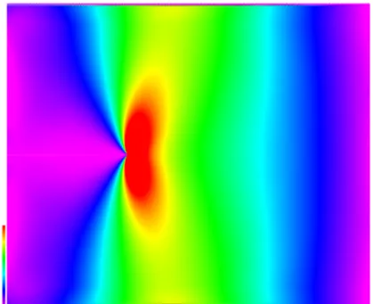
Computer simulation of material fracture can be computationally expensive due to the large number of elements necessary to capture microstructue features. One example of such material is nacre and its synthetic analogues, which has a mechanical response that depends strongly on the microstructure features. Explicit representation of these features can lead to very large problem sizes, for which simulations can require substantial computation time. In these materials, individual “bricks” interact with each other through a polymer that binds the bricks. The problem size discussed in this dissertation can reach up to 300,000 bricks. Figure 1.1 shows an example simulation output. In the figure, the colors represent vertical brick stress.
Figure 1.1. An example simulation output. The colors represent vertical brick stress.
One way to model the problem is to use rigid elements with interfaces that can fracture, under a quasi-static loading scenario. In this case, the problem can be solved by using global Monte Carlo minimization algorithms to minimize the energy of the system, which comes from the deformation and fracture of the interfaces under external loading. To alleviate the high computational cost of these simulations, we have developed GPU-
(Graphics Processing Unit) based Monte Carlo minimization algorithms that achieve significant speedup over conventional CPU-based algorithms. 22,24,25,26 GPUs offer a highly parallel computational resource that can substantially increase the performance of algorithms that can take advantage of it. The details of the algorithms will be described later in the dissertation.
Another, more complicated way to model the problem is to use deformable elements with interfaces that can fracture, using an explicit time discretization. In this case, the
implicitly. We have developed explicit, CPU-based methods as well as implicit-explicit methods on both CPUs and GPUs. We describe the details of these methods later in the dissertation.
The remainder of this dissertation is organized as follows. In Chapter 2, we discuss GPU-based Monte Carlo minimization algorithms for rigid elements. In Chapter 3, we present an improved GPU implementation of AES (Advanced Encryption Standard), which is used to generate random numbers that are required for the Monte Carlo minimization
algorithms. In Chapter 4, we describe our implementation of explicit methods, and show how an implicit-explicit time-stepping method can be very well-suited to problems with
Chapter 2 High-performance simulation of fracture in idealized “brick and mortar” composites using adaptive Monte Carlo minimization on the GPU
Simulations of fracture that explicitly account for material microstructure can be enormously expensive, due to the fact that large numbers of degrees of freedom are necessary to capture the effect of individual microstructure features. An excellent example of this challenge is the simulation of fracture in nacre and its synthetic analogues, which consist of small ceramic platelets bonded together with a very small volume fraction of polymer. The mechanical response of these materials is strongly influenced by the dimensions and arrangements of the platelets, and explicit representation of all features in the microstructure within the fracture process zone leads to daunting problem sizes, as a high density of discretized elements is required.10,11,14 Further, the strong interaction between the fracture process and the brick arrangement implies that fracture pathways are not known a priori, creating the need to allow for arbitrary cracking pathways to evolve with loading.12,19 The need to capture local material rupture (e.g. the breaking of bonds holding platelets together) further compounds the
problem, as rupture represents a strong nonlinearity that produces sharp spatial gradients in stiffness (i.e. a crack has zero stiffness while the surrounding material may be intact and therefore have high stiffness). For such problems, methods that rely on gradient-based techniques to find the roots of non-linear equilibrium equations are often prone to extreme convergence difficulties that stem from the sharp discontinuities in stiffness.
We present an idealized model for nacreous materials that represents the platelets comprising the microstructure as rectangular bricks, whose position and orientation are solution variables to be determined through simulation. The bricks interact through
non-linear springs, which represent the very small volume fraction (1-5%) of polymer mortar that hold the bricks together.13,20,21 Hence, the non-linear spring description represents the
constitutive law that describes mortar, and includes both elastic response (for small separations between bricks), plastic response (when the separation between bricks causes straining of the mortar beyond its elastic limit), and rupture (when the separation between bricks is large enough to cause material failure in the mortar). Figure 2.1 provides a schematic illustration of the material model. A companion paper more fully discusses the physical justification and implications of the model, using the solution techniques and algorithms described here to quantify fracture parameters controlling failure.22
Noting the fact that many fracture problems involve limited amounts of unloading, the problem can be cast in terms of energy minimization of a non-linear elastic system: in this case, described by the non-quadratic energy potential describing the springs, or mortar. We treat the bricks as rigid due to their extreme stiffness relative to that of the mortar, thus the problem is essentially that of a collection of nearest-neighbor particle interactions.22
The end result is a material idealization that simply involves finding the collection of brick positions and rotations that minimize the energy in the non-linear springs connecting the particles. From a purely mathematical point of view, this is a fairly general problem in that it involves finding global energy minima of a highly nonlinear system of nearest neighbor interactions. While the idealized material model described above serves as the motivation, the algorithms described here are applicable to other problems of this type (such as the large deformation of fiber networks22). The focus of this chapter is on the strategic marriage of the GPU architecture to this class of problems. We will show that the GPU
architecture offers powerful advantages, particularly when combined with algorithms that exploit the nature of nearest-neighbor interactions. Results are presented quantifying computational performance. This work appeared in24. For additional details regarding the material aspect of the simulations, see 22,25.
2.1 Background 2.1.1 Model
Figure 2.1. (a) Schematic of macroscopic specimen and loading scenario (bending). There is a pre-existing crack in the middle of the specimen. (b) An example configuration of bricks. Many more bricks are used in the actual simulations. (c) Assignment of bricks to threads using graph-coloring. Adjacent bricks are assigned different colors. Bricks of the same color are processed in parallel.
The central objective of the simulations presented here is to predict failure of a macroscopic specimen that has a large, pre-defined crack and is loaded in a combination of tension and bending, as shown in Figure 2.1(a). The macroscopic specimen is created by defining a two-dimensional “wall” of overlapping rectangular bricks that are connected with cohesive springs; Figure 2.1(b) shows a close-up view of this microstructure and the dimensions that define the bricks. The bricks are treated as rigid bodies, while the mortar (implicitly
represented by the cohesive springs connecting the bricks) is described as a nonlinear material. A large number of bricks are used to accurately capture the complex fracture behavior near the tip of the macroscopic crack shown in Figure 2.1(a). The simulation tool has been coded to allow for arbitrary combinations of brick width, height, overlap, and orientation within a specimen. (Here, example results are presented for a single
microstructural orientation relative to the specimen; more exhaustive study of the role of brick size and orientation is presented in a separate work.22)
The specimen is loaded by applying prescribed displacements to the bricks at the top and bottom of the specimen shown in Figure 2.1(a). Bricks without prescribed displacements can undergo general rigid body motions (translation and rotation). As the bricks displace and rotate, the interface opening between bricks can change. The cohesive law describes the energy that is stored at the interfaces as the bricks change position, in terms of the relative displacements between the adjacent bricks defining the interface. The cohesive description contains three parameters: interface stiffness, critical separation, and work to failure. The energy of an interface is computed as follows
Einterface=
∫
Eptds (2.1)where the integral is over the length of the interface. The energy at a given point is given by
Ept=f(
√
∆n2 +∆t2)+g(∆n) (2.2)
where Δn is the displacement in the normal direction and Δt is the displacement in the tangential direction, and f and g are given by
f(x)=
{
0.5 k x2, x≤x1 k x1(x−0.5x1), x1<x≤x2 −0.5k [x12+x22+x2−2x (x1+x2)], x2<x<x1+x2 k x1 x2, x≥x1+x2 (2.3) g(x)={
0, x≥0 0.0625 k x2(
x x1)
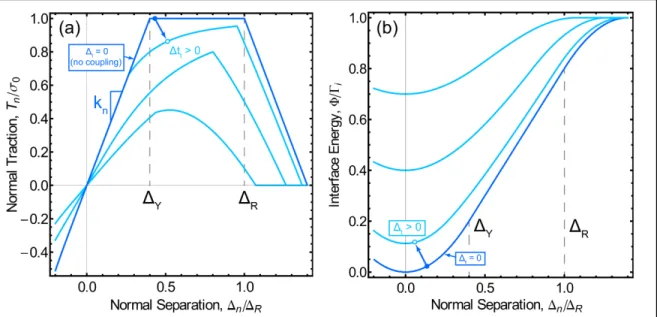
4 , x<0 (2.4) where k is the interface stiffness, x1 is the critical separation, and k x1 x2 is the work tofailure. The traction generated between bricks is simply the derivative of the cohesive energy potential with respect to relative displacements. Figure 2.2 illustrates the traction-separation relationship as a function of brick separations, and the associated energy potential. At small relative displacements, the tractions are linear with separation, representing the elastic phase of mortar response: above a critical displacement, the traction remains constant, representing the plastic yielding phase of mortar response. The rupture separation defines the point at which the mortar begins to fail: for large relative displacements, the traction between bricks is zero, and the energy potential assumes the value of the area under the traction-separation curve.
Figure 2.2. (a) Graph of traction-separation function. (b) Graph of the energy potential, defined as the integral of the traction-separation function.
2.1.2 Basic Numerical Method
The simulation is thus an energy minimization problem, where the solution involves finding
x1,y1,θ1,x2,y2,θ2,....xn,yn,θn, where xn,yn,θn is the x-position, y-position, and orientation of brick
n, such that the energy E(x1,y1,θ1,x2,y2,θ2,....xn,yn,θn) is minimized. The energy function E
depends on the brick size and orientation and the properties of interfaces between bricks. For problems involving cohesive yielding or rupture, the energy landscape is multidimensional, highly non-linear, and may contain several solutions (local minima). For problems of this nature, typical gradient based schemes do not perform well; instead, direct heuristic search numerical optimization algorithms are preferred. We use the Monte-Carlo direct search method, also known as simulated annealing, to find the minimum.15,16,18 In this case, the temperature parameter T is a fictitious parameter that is chosen by the user, as opposed to a physically meaningful temperature used in annealing simulations involving physical quenching.
One advantage of simulated annealing is that it is highly parallelizable, which allows us to leverage the computational power of GPUs. The basic parallelization concept is to move multiple bricks simultaneously, computing the associated energy change and accepting those that lower the energy. A small fraction of movements that increase the energy are accepted as well, to avoid being trapped in a local minima; an exponential function is used to describe the probability controlling the acceptance of movements that raise energy. In this approach, one must avoid moving adjacent bricks at the same time; as will be described, we address this problem by coloring the bricks using a graph coloring algorithm to identify sets of non-adjacent bricks, as shown in Figure 2.1(c). Different sets of bricks, each with a given color, are passed into separate threads of the GPU.
The basic algorithm is outlined as follows. While the solution for any given
prescribed displacement can be found in a single minimization step, in the approach taken here, the prescribed displacements are applied incrementally. This both captures solutions at a range of loads and promotes convergence, as described in subsequent sections:
Apply displacement mi to each driven brick dk Repeat these steps until convergence
For each free brick bn, perform the following steps: Compute the current energy Eold
Generate standard uniform random numbers rx, ry, rθ Perturb the position and orientation using rx, ry, rθ Compute the new energy Enew
Accept the new position and orientation Else
Generate a standard uniform random number r If r < exp( (Eold - Enew) / T)
Accept the new position and orientation Else
Reject the new position and orientation
2.2 Adaptive Numerical Methods
We have developed and implemented several enhancements to increase performance and usability of the basic algorithm. These methods include adaptive cycle count, adaptive step size adjustment, adaptive displacement adjustment, and a position predictor.
The adaptive cycle count allows the user to specify tolerance values. The algorithm will run as many iterations (cycles) as necessary to reach the specified tolerance values. Without this, the user would have to specify cycle count directly, but the number of cycles required to converge is not known beforehand.
Figure 2.3. (a) Adaptive cycle illustration. The old sliding window is labeled windowold,
while the new sliding window at the next cycle is labeled windownew. The blue circle is the
new energy value, and the red circle is the old energy value. The variance and correlation coefficient are calculated each time the sliding window is updated. (b) Graph of position predictor multiplier. The predictor uses linear prediction when the energy is low, and a combination of linear and constant prediction as the energy increases.
The underlying idea is illustrated in Figure 2.3(a). We use a sliding window to monitor the variance and correlation coefficient to determine convergence. At each cycle, the new energy value is added to the sliding window (blue in Figure 2.3(a)), while the old value is removed (red). Then the variance and correlation coefficient of the window are calculated and compared to user-specified tolerance parameters. These tolerance parameters include WS (size of the sliding window, which corresponds to the number of Monte Carlo cycles), STOL (tolerance for variance), RTOL (tolerance for correlation coefficient), and ConvergenceRep (the number of times the convergence criteria need to be met to advance to the next
displacement step). After the STOL and RTOL criteria have been met for ConvergenceRep times (which is typically set to 1/4 to 1/2 of WS), the current displacement step is considered to be finished.
There are several methods to calculate the correlation coefficient and variance. One approach is to use a two-pass algorithm that calculates the mean first and then calculates the variance. This approach does not work well for this situation since whenever a new value is added or an old value removed from the sliding window, the entire window has to be reprocessed. A different approach is to use a one-pass algorithm that dynamically updates without reprocessing the entire window. A well-known formula is the following 9
SQnew=SQold+x2new−xold2 ; SQinit=0
SNnew=SNold+xnew−xold; SNinit=0
variance=
SQnew−SNnew
2
WS
WS (2.5)
where xnew is the new value, xold is the old value, WS is the window size, and SQ and SN are
intermediate variables.
However, this formula suffers from round-off errors and the computed variance can become negative rather quickly. We use a more numerically stable one-pass formula 9
meannew=meanold+xnew−xold
WS ; meaninit=0
SSnew=SSold+(xnew−meannew)(xnew−meanold)−(xold−meannew)(xold−meanold); SSinit=0
CSnew=CSold+(xnew−meannew)(
WS+1
2 )+(xold−meanold)(
1−WS 2 ); CSinit=0 variance=SSnew WS R2= CSnew 2 WS∗variance∗(WS 2 −1 12 ) (2.6)
where variance and R2 (correlation coefficient) are the output values, and mean, SS, CS are the intermediate variables.
This formula accumulates round-off errors more slowly than the previous formula, but it can still produce a negative variance after some time. To remedy this problem, the MPFR
package 8 was used to compute the intermediate values (mean, SS, CS) at quadruple
precision, whereas normal floating-point numbers are either single or double-precision. The MPFR package is a widely used library for performing extended precision calculations. After the variance and R2 are computed, they are compared to the user-specified STOL and RTOL criteria to determine convergence.
We included an adaptive step size strategy that modifies the brick step size (the amount of perturbation to a brick's position during one step) and rotation size (the amount of perturbation to a brick's orientation) based on acceptance probability.17,23 If the acceptance probability is very low, then most of the attempted moves are rejected, which results in a loss of efficiency. If the acceptance probability is very high, then this implies that the brick step size and rotation size is small, so it would take more time to converge after an applied displacement. The equation for adjusting both the brick step size and rotation size is given by
sn+1=
{
sn∗(0.5+α), α<0.4,α>0.6sn, 0.4≤α≤0.6 (2.7)
where sn is the step size at load step n, and α is the acceptance probability. The step size can
be adjusted either globally or on a per-brick basis. In global adjustment, a single step size is used for all bricks and adjusted periodically. For the per-brick basis, each brick maintains its own step size.
Our strategy for adaptive displacement adjustment controls the displacement size to reach stable crack growth behavior. The displacement size is adjusted using forward control
and backtracking. In forward control, the step size is adjusted proportionally based on a target number of cycles for convergence. The equation for forward control is given by
Δn+1=Δn∗ct
cr (2.8)
where Δn is the displacement step size at load step n, ct is the target number of cycles and cr is
the actual number of cycles required to converge the previous displacement step.
Besides forward control, we also use backtracking, which occurs when the number of cycles exceeds an upper limit. In backtracking, the displacement step is reverted and the new displacement step size is given by
Δn+1=Δn∗2
3∗
ct
cu (2.9)
where cu is the upper limit for cycles.
A position predictor is used during the early stage of the simulation (prior to
widespread rupture between bricks) to accelerate convergence, since the relationship between prescribed displacements and brick positions is approximately linear. In this case, the
converged position of the bricks in one displacement step is linearly extrapolated to obtain an initial position for the next displacement step that results in a faster convergence. The
predictor is given by pin+1 =pin +Δn+1 Δn ∗
[
pin −pin−1]
∗m (2.10) where pinis the position of brick i at displacement step n, and m is the multiplier defined
As the simulation progresses, the interfaces between bricks approach the point of fracture, where a linear predictor is no longer accurate, and a constant predictor is more appropriate. To reduce the prediction error, the following multiplier is used
m=1−1.8
(
[
max(
min(
ΦΦ0,1.0
)
,0.5)
]
−0.5)
(2.11) where Φ is the current brick energy, and Φ0 is the maximum elastic brick energy.
As shown in Figure 2.3(b), when the brick energy is low, the multiplier is equal to 1, so the linear predictor is used. As the brick energy increases, the multiplier value decreases, resulting in the use of a linear combination of constant predictor and linear predictor. The position predictor results in a significant performance improvement during the harmonic (non-fracture) part of the simulation, as will be discussed subsequently.
2.3 GPU Architecture
During the past few years, GPUs have increasingly been employed for scientific and engineering computations as GPU architectures have become more flexible and powerful.1 To achieve high performance on the GPU, it is important to understand the differences between CPU and GPU architectures, which are illustrated schematically in Figure 2.4. A general-purpose CPU, such as the Intel Core i7-2600 or the AMD Phenom II X6 1100T has several cores to run multiple threads (4 physical cores / 8 virtual cores for the Core i7-2600 and 6 physical cores for the Phenom II X6 1100T). It also has a large cache (8MB for the Core i7-2600 and 6MB for the Phenom II X6 1100T). A CPU also has sophisticated flow control mechanisms, such as branch prediction, data/instruction prefetching, out-of-order
execution, and superscalar execution. CPUs are designed to run a few threads as fast as possible, and are well-suited for problems with a low degree of parallelism.
In contrast, a GPU, such as the Nvidia GTX 580 or the AMD Radeon HD 6970, has a large number of execution units to process a large amount of data in parallel. For example, the Nvidia GTX 580 has 16 SMs (Streaming multiprocessors), where each SM has 32 SPs (Shader processors). Each SM can execute independent streams of instructions, whereas the SPs within each SM execute instructions in a SIMD (Single Instruction Multiple Data) manner. The Nvidia GTX 580 has a 64K L1 cache and a 768K L2 cache. GPUs lack the sophisticated flow control mechanisms that are present on CPUs, such as branch prediction. GPUs are designed to run large numbers of threads, and are suited for problems with a high degree of parallelism.1,2
In comparing CPU and GPU, a GPU has many more transistors devoted to execution units than a CPU, whereas a CPU has more transistors devoted to cache and flow control mechanisms compared to a GPU, as shown in Figure 2.4.
Figure 2.4. CPU and GPU architectures. A GPU has more transistors devoted to execution, while a CPU has more transistors for cache and control mechanisms.
The result is that a GPU can reach higher peak performance, as shown in Figure 2.5, which compares flop rates and bandwidths of Nvidia GPUs and Intel CPUs. Figure 2.5(c) shows the double-precision FLOP rate on the two GPUs and two CPUs used for the test system.
Figure 2.5. (a) Peak GFlops of CPUs and GPUs. The peak GFlops is significantly higher on a GPU. (b) Peak memory bandwidth of CPUs and GPUs. The peak bandwidth is significantly higher on a GPU (c) Peak double precision GFLOP/s on the test systems: Nvidia GTX 480 GPU/Core 2 Quad Q6600 CPU and Nvidia GTX 580 GPU/Core i7 2600 CPU.
To approach the peak performance of the GPU, the code needs to be structured in a way that takes advantage of the architecture of the GPU and avoids the limitations that reduce performance. These considerations include having enough threads running in parallel, ensuring coalesced memory access, minimizing data transfer between GPU and CPU, and minimizing warp divergence.1,3
Having enough threads running in parallel is important because GPUs are designed for highly parallel operations, which allows latency in one thread to be hidden by performing other operations in another thread. In addition, context switching between threads on a GPU is significantly less expensive than on a CPU.1 For these reasons, it is typical to have
Ensuring coalesced memory access improves performance since the memory controller on a GPU performs operations based on groups of threads at a time. Memory access is coalesced when the threads within a group access a contiguous region of memory. For example, the Nvidia GPU uses a warp of 32 threads.1 If the memory access within a warp is not coalesced, then the controller must perform additional operations, which reduce performance.
Minimizing data transfer between the GPU and the CPU is another important consideration. The bandwidth of the link between CPU and GPU is much lower than the on-board memory in the GPU. For example, the Nvidia GTX 580 has a 16x PCI-Express 2.0 capable interface, which can transfer a maximum of 8 GB/s between CPU and GPU. In contrast, the on-board memory on the GTX 580 has a maximum transfer rate of 192.4 GB/s, which is much higher.
Minimizing warp divergence is important since GPUs operate in a SIMD manner. Warp divergence is caused by different threads taking different execution paths, such as two threads taking different branches in a conditional statement. Whenever the GPU encounters warp divergence, it serializes the execution of the warp, which leads to reduced
2.4 GPU Implementation
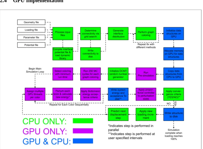
Figure 2.6. Flowchart of the overall simulation algorithm.
Prior to the GPU-based simulation algorithm, input processing and initialization steps are performed on the CPU. An overview of the CPU and GPU operations in the present code is shown in Figure 2.6. The input processing step reads information about the bricks, interfaces, and the overall structure from input files. This step allows the simulation to handle different brick shapes and sizes, and different interface properties. In the data structure, each brick has a position, orientation, constraints, neighbor information, and interface properties associated with it.
The initialization step involves finding the connectivity between bricks and
find the interface connectivity, with a time complexity of O(N). The algorithm works by setting up a rectangular grid of cells and associating each brick to a cell. Then it finds all candidate bricks that are within a certain distance of the selected brick and tests them for interface connectivity, i.e. whether two bricks have a common interface. We then use a graph-coloring based algorithm to determine which bricks can be processed in parallel.15 Neighboring bricks are colored with different colors, then all bricks with the same color are grouped together. Figure 2.1(c) provides a diagram that illustrates the graph coloring. Adjacent bricks cannot be processed in parallel since this would result in a data race. After these steps have been performed, the data structure containing information about bricks and interfaces is transferred to the GPU memory. The number of bricks that can be simulated is limited by the amount of GPU memory; with the GTX 580, we can simulate up to 2,000,000 bricks. Next, the pre-simulation phase is performed. In this phase, the different candidate graph colorings from the previous phase are used to execute the simulation for a small number of cycles. The reason for performing pre-simulation is because in general, the graph coloring problem is NP-complete. As a heuristic, we generate several possible candidate colorings and determine their execution time. The execution time can vary for different colorings because different colorings generate different memory access patterns. It is difficult to know a priori which coloring will be optimal. The graph coloring that minimizes the execution time is selected for the main simulation phase.
At set intervals chosen by the user, some state information is transferred from GPU to CPU so that intermediate states can be obtained by the user. The majority of the data remains
on the GPU to minimize the amount of time spent in transferring data across the bus since the bus is much slower than the on-board memory of the GPU.
The random numbers that are used in simulated annealing are generated via a two stage process. First, parallel, independent streams of random numbers are generated using the Dynamic Creation Mersenne Twister (DCMT) algorithm.4 Having independent streams ensures that there is no correlation between the different streams that could potentially skew the simulation results. Each stream of random numbers is associated with a different set of generator parameter values, which we computed on a cluster. The parameter values are computed once and can be reused multiple times with different seeds to generate different sets of independent streams of random numbers. The original DCMT algorithm was written to run on a CPU.4 The DCMT algorithm was modified by NVIDIA to run on the GPU using CUDA.5 We have further modified the DCMT algorithm to improve its initialization and increase randomness. Rather than using one seed value for all the random number generators (RNG), we modified the process to generate multiple seed values from the initial seed, one for each RNG. We have also improved performance by increasing thread parallelism and exploiting instruction pipelining. Then, the output is processed using Advanced Encryption Standard-Electronic Codebook (AES-ECB) 6 to improve the randomness properties. We have parallelized the AES algorithm to run on the GPU. We used TestU01, which contains a large collection of statistical tests for random number generators, to test the quality of our random number generation.7 In TestU01, the Mersenne Twister passed all tests except for the linear complexity tests. Processing the output of MT using AES enables the results to pass all of the statistical tests in TestU01.
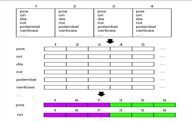
In the simulation, bricks are assigned to threads using a graph-coloring based algorithm since neighboring bricks cannot be modified simultaneously. For example, in Figure 2.1(c), bricks 1 and 6 are non-adjacent and colored purple, while bricks 2 and 4 are colored blue, and so on. Then all of the purple bricks are processed in parallel, followed by all of the green bricks, and so on. During the simulation, thousands of threads are launched to simulate a large number of non-adjacent bricks in parallel. This takes advantage of the large number of execution units available on a GPU. However, it also leads to a less coalesced memory access pattern since the bricks are non-adjacent, which reduces performance. To overcome this issue, we rearranged the data structure on the GPU so that the memory access pattern is more coalesced. During input processing, the data is stored in array of structure format. In an array of structure format, an object's properties are grouped together. This format is used because the data structure needs to change dynamically as input files are processed. Afterward, the data is rearranged into a structure of array format for computation on the GPU since this is more efficient. In a structure of array format, properties of the same type from multiple objects are grouped together. In addition, the order of the individual elements in the data structure are rearranged to increase efficiency. The rearrangement is performed once on the CPU, prior to the main simulation phase. Figure 2.7 provides a diagram of the data structures used in the simulation.
Figure 2.7. Diagram of the data structures used in the simulation. Initially, the data structures are in an array of structure format during input processing. It is then rearranged into a structure of array format. Additionally, the individual elements are rearranged according to the graph coloring order.
2.5 Results
The test problem discussed below has the following configurations. The bricks are oriented with varying angles with respect to the macroscopic crack direction, and the bricks have a width to height ratio of approximately 3.5. The number of bricks in various simulations ranges from approximately 50,000 to 350,000. The bricks are displaced under a bending scenario, as shown in Figure 2.1(a). The parameters used in the simulations considered here are listed in Table 2.1.
Table 2.1. Parameters used in the results section.
STOL = 0.002 RTOL = 0.03 ConvergenceRep = 1500 WindowSize = 3500 DumpInter = 10e0 AdaptInter = 5e3 TEMP = 0.00075 InitialStepSize = 0.001 MinStepSize = 0.0001 MaxStepSize = 0.02 InitialRotSize = 0.001 MinRotSize = 0.0001 MaxRotSize = 0.02 AmpFactor = 1 InitialLoadStepSize = 0.02 MinLoadStepSize = 0.005 MaxLoadStepSize = 0.08 StructSteps = 1 WindowMul = 20 WindowUpperMul =50000 STOL = 0.002 RTOL = 0.03 ConvergenceRep = 1500 WindowSize = 3500 DumpInter = 10e0 TEMP = 0.00075 InitialStepSize = 0.001 MinStepSize = 0.001 MaxStepSize = 0.001 InitialRotSize = 0.001 MinRotSize = 0.001 MaxRotSize = 0.001 AmpFactor = 1 InitialLoadStepSize = 0.02 MinLoadStepSize = 0.02 MaxLoadStepSize = 0.02 StructSteps = 1
The test problem was run on two different platforms to compare performance. The first platform consists of a Core 2 Quad Q6600 CPU at 2.4 GHz, EVGA nForce 780i motherboard, 8GB DDR2-800 memory, and an Nvidia GTX 480 GPU. The second consists of a Core i7 2600 CPU at 3.4 GHz, Gigabyte Z68X motherboard, 16GB DDR3-1333 memory, and an Nvidia GTX 580 GPU. The software environment is CentOS 6, GCC 4.4, and CUDA runtime 4.0.
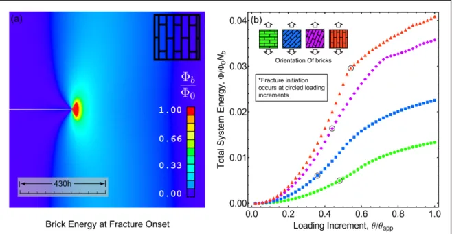
Figure 2.8. Simulation output. (a) The colors represent the energy of the bricks. (b) The total energy for various brick orientations.
Figure 2.8 provides an illustration of the results obtained from the simulation; the energies associated with the interfaces surrounding a given brick are shown in Figure 2.8(a), while the relationship between global system energy and the prescribed loading is shown in Figure 2.8(b). In Figure 2.8(a), the bricks near the crack tip have high energy due to the significant stress concentration of the crack tip, and the bricks farther away have lower energy. The region shown in red in Figure 2.8(a) represents the fracture process zone where the interfaces between bricks are experiencing failure; at greater loads, the macroscopic crack advances, meandering between bricks according to the microstructural orientation. Extensive details of the fracture process are provided in our companion paper.22
Figure 2.8(b) illustrates that for small levels of applied displacement, the system energy is essentially quadratic, as implied by a linear (elastic) traction-separation
quadratic nature of the energy with loading is lost, due to nonlinear rupture effects between the bricks. The solutions for displacements below the onset of rupture are obtained in a rapid fashion using the predictor method described earlier. Once fracture initiates, the linear predictor is less efficient, so the constant predictor becomes more appropriate.
A key consideration in this simulation approach is the scaling of the required
computation times with the number of bricks, which effectively defines the size of problem (i.e. the level of microstructural detail) that can be simulated in a reasonable time.
Figure 2.9. (a) Initialization time. (b) GPU and CPU simulation times (semilog).
As shown in Figure 2.9(a), the initialization time scales approximately as O(N), where N is the number of bricks. The initialization is done on a single core. Both the Core 2 and Core i7 are quad-core processors, but the Core i7 has a more modern architecture (Sandy Bridge for Core i7 vs Conroe for Core 2) and a faster clock speed, so the result is faster on the Core i7. In addition, the Core i7 system also has faster and larger memory.
After initialization, the main part of the simulation begins. These cases are run with the adaptive methods. The simulation times for the two different systems are shown in Figure 2.9(b). We can see that on the first system (GTX 480 and Core 2), the GPU version (GTX 480) is about 16 times faster than the corresponding multithreaded CPU version (quad-core Core 2), whereas on the second system (GTX 580 and Core i7), the GPU version (GTX 580) is about 6 times faster than the multithreaded CPU version (quad-core Core i7). The
simulation time scales roughly as O(N1.5), where N is the number of bricks. The simulation time for GTX 580 is approximately 15% faster than for GTX 480, which roughly matches the hardware performance difference between GTX 480 and 580. The simulation time for Core i7 is approximately 3 times faster than for Core 2. Both processors are quad-core, but the Core i7 has approximately 40% higher clock speed and a newer architecture.
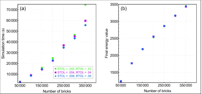
Figure 2.10. (a) GPU simulation times with different tolerance values. (b) Final energy value with different tolerance values.
In Figure 2.10(a), the simulation times for different RTOL and STOL are shown. The simulation times for larger tolerance values are generally lower; however, there is some
variability due to the stochastic nature of Monte Carlo simulations. In Figure 2.10(b), the converged energy values at the last displacement step are shown for different tolerance values. Simulations with smaller tolerance values generally result in slightly lower energy values, although all three tolerance values produce energy values that are quite similar.
Figure 2.11. CPU simulation time with different numbers of cores.
As seen in Figure 2.11, the simulation time on the CPU scales approximately in a linear manner with the number of cores. This indicates that the CPU implementation is not experiencing scalability bottlenecks that would limit performance, at least up to four cores.
Figure 2.12. Percentage of simulation time for different parts of the algorithm on GTX 480 and 580.
To determine which tasks of the computation take the most time, Figure 2.12 shows the percentage of the total simulation time for the main tasks in the simulation. As seen in the figure, the Monte Carlo task takes the largest percentage of the simulation time. The Monte Carlo component involves perturbing the position and orientation of each brick, and
determining whether to accept or reject based on the energy difference. The other two components, which are the energy calculation and the random number generation, take significantly less time, with the random number generation being the smallest component. The random number generation component generates random numbers which are then used in the Monte Carlo component. The relative percentages remain roughly constant with respect to the number of bricks, which is expected. The percentages are also similar across the two GPUs (GTX 480 and 580). These three components take 99% of the simulation time. The reason that the Monte Carlo component takes a significant portion of the simulation time
is that it involves non-coalesced memory access. We have optimized the data structure to reduce the amount of non-coalesced memory access, but some of it still exists.
2.5.1 Performance improvement due to adaptive methods
In this section, the test problem is the same as in the previous section, but the simulation has been run without the adaptive methods to illustrate the difference in performance. Figure 2.13 provides a comparison of simulation times with and without adaptive methods for two GPUs, both in terms of raw values (Figure 2.13(a)) and relative performance (Figure 2.13(b)).
Figure 2.13. (a) Comparison of GPU simulation time for adaptive vs. non-adaptive algorithms. (b) Relative speedup from using GPU and adaptive methods. The time for Core 2 Quad Q6600 non-adaptive is an estimated runtime based on the difference between GTX 480 adaptive and GTX 480 non-adaptive, and the difference between GTX 480 adaptive and Core 2 Quad Q6600 adaptive, since it takes an impractical amount of time to run the Core 2 non-adaptive case.
From Figure 2.13(a), the performance difference between running with the adaptive algorithms and without the adaptive algorithms is about a factor of five. The position
predictor produces the largest improvement in performance. Other adaptive methods, such as adaptive brick step size and adaptive displacement size, also produce some improvements in performance, but not as large as that of the position predictor. The performance gain from adaptive methods is problem dependent; in some cases, the improvement can be much higher. For example, if a large proportion of the simulation is harmonic, then the adaptive methods can result in significantly larger speedups.
Figure 2.13(b) summarizes the speedup we have achieved through efficient GPU implementation and adaptive strategies. As seen in the figure, our GPU implementation achieves approximately 16x speedup over the multithreaded CPU (quad-core)
implementation for the test problem with 300,000 bricks, and the adaptive methods achieve an additional 5x speedup, for a total speedup of about 80x. This is a significant speed-up that will have a marked impact on studies of microstructural effects.
2.6 Conclusion
In this chapter we have presented an efficient GPU-based Monte Carlo algorithm for fracture simulation of large-scale “brick and mortar” composite materials. We have enhanced the basic algorithm with adaptive methods to increase performance and usability. Our GPU implementation processes multiple bricks in parallel using graph-coloring to assign bricks to threads. Our GPU version achieved approximately 16x speedup over the corresponding
multithreaded CPU (quad-core) version. An additional 5x speedup was achieved using adaptive algorithms, for a total speedup of approximately 80x. This enables a simulation to be run in hours on a GPU as opposed to weeks on a CPU.
Chapter 3 Bitsliced High-Performance AES-ECB on GPUs
The purpose of this chapter was to develop fast methods for generating deterministic random numbers using the AES in the ECB mode. The resulting random numbers were intended to be used in high-performance Monte Carlo simulation of fracture in certain composite materials.24 The simulations for this study were done both on CPUs and GPUs to obtain the fastest implementations, and thus, to compare the speedup gain. We were motivated to develop high-speed implementations of the 128-bit AES-ECB on the NVIDIA GTX 480 GPU, and subsequently obtained significantly faster implementations of the AES. This chapter reports our implementations along with comparisons to recent results found in the literature. This work appeared in 26.
3.1 Comparing GPUs
The GTX 285 has 30 SMs, each with 8 SPs. It has 16K L1 cache per SM and no L2 cache. It also has 16384 registers per SM and 1 GB of global GPU memory. In comparison, the 8800 GTX has 16 SMs, each with 8 SPs. It has 16K L1 cache per SM and no L2 cache. It also has 8192 registers per SM and 768 MB of global GPU memory.
We find it useful to make a comparison of various GPUs that we are referencing in the context of our AES implementations. Table 3.1 compares various GPUs referenced in this paper. Here, CC refers to “Compute Capability”, which is an index assigned by NVIDIA to the CUDA devices to indicate its set of computation-related features. Higher CC indicates newer architectures, and the NVIDIA’s newest devices have a CC up to 3.540
8800 GTX41 GTX 28542 Tesla C205044 GTX 48043 bus bandwidth 4 GB/s 8 GB/s 8 GB/s 8 GB/s memory size 768 MB 1024 MB 3072 MB 1536 MB mem bandwidth 86.4 GB/s 159.0 GB/s 144 GB/s 177.4 GB/s SP count 128 240 448 480 SP clock 1350 MHz 1476 MHz 1150 MHz 1400 MHz CC 1.0 1.3 2.0 2.0
3.2 AES Encryption on CPU and GPUs
Since the standardization of the Rijndael algorithm as the Advanced Encryption Standard by NIST6, many implementations have been reported in the literature, most of which rely on known techniques. The creators of the Rijndael algorithm describe two fundamental
techniques for 8-bit and 32-bit CPUs. 30 The most common use of the AES is for the 128-bit (16-byte) key; it is projected that AES will be 40% slower27 for 32-byte keys since it uses 14 rounds, instead of 10.
Furthermore, there are several modes of operation: the CBC (cipher-block chaining), the ECB (electronic code-book), the OFB (output feedback), and the CTR (counter) modes, etc. Moreover, there are several ways of benchmarking the AES software, making a fair comparison very difficult. Most common comparisons involve AES-ECB and AES-CTR modes. We refer the reader to a highly useful paper by Bernstein and Schwabe27 that gives extensive analyses of various implementations, along with the most impressive benchmark results.
Earlier GPU implementations29,31,49 used graphics pipeline and OpenGL to compute the AES round function, since CUDA was not available back then. The availability of CUDA made sophisticated high-speed implementations possible.
Another point of discussion that is relevant here is bitsliced AES implementations on various CPUs. There are several papers of interest: Rebeiro, Selvakumar and Devi48,
Matsui37, and Matsui and Nakajima38. Bitsliced implementations are not as competitive with word-level implementations on CPUs, due to the cost of transpositions of the ciphertext.
3.3 AES-ECB on the GPUs
Our implementation starts with the CPU-based bitsliced implementation of the AES by Kasper and Schwabe.34 Their implementation processes 8 16-byte blocks at a time. A direct conversion to a GPU implementation results in poor performance, due to an insufficient number of registers. The 8 blocks alone take up 32 registers per thread, and each thread is limited to 63 registers maximum. The result is that the compiler spills variables into memory instead of keeping them in registers.
We restructured the algorithm to process 4 16-byte blocks at a time to improve performance. The sections below describe the performance improvements we made to various parts of the AES algorithm.
3.3.1 Bit Ordering
In our bitslicing implementation, bits from multiple blocks are collected together, i.e. bit 0 of row 0, column 0 from blocks 0,1,2,3 are grouped together, as shown in Figure 3.1 and Figure 3.2. Each bitsliced state variable has 64 bits; there are 8 of these state variables.
Figure 3.1: The state of one block.
Figure 3.2: The bitsliced state.
3.3.2 Load and Store
On GPUs, the performance of global memory is improved when it is accessed contiguously. When reading the input blocks, we first load the blocks contiguously from global memory to shared memory, and then distribute them among individual threads. Similarly, when writing the output blocks, we first write the blocks to shared memory from individual threads, and then collect them together and store to global memory contiguously.
3.3.3 SubBytes
The AES algorithm defined in 6 used a table lookup for the S-box. In the bitsliced implementation, the table lookup is replaced by a series of Boolean operations (xor, or, and).34 Kasper and Schwabe34 used 163 CPU SSE instructions. In our implementation, since we restructured the algorithm to process 4 blocks at a time, extra registers are available that
we use to store intermediate values, thus reducing the instruction count to 11 7×2 . The doubling of the instruction count arises from the fact that the GPU registers are 32 bits, thus, each 64-bit bitsliced state requires 2 operations to process. Since the two halves can be processed independently, we utilize ILP (instruction level parallelism) to increase performance.
3.3.4 ShiftRows
In this step, the bytes in a block are shifted by a variable amount for each row, as shown in Figure 3.3. In the bitsliced state, this operation becomes a rearrangement of nibbles (4-bits), as shown in Figure 3.4. The CPU version used the pshufb instruction34, but this instruction is not available on the GTX 480. Instead, we found the GTX 480 has a prmt instruction that rearranges bytes.45 We combined this instruction with the standard C bit operations (>>,
<<, &, |, ^) to improve performance. The CPU version uses 8 SSE instructions34, while
our GPU version uses 32 prmt, 16 shift, and 16 bitwise and instructions. The GPU version requires more instructions since it involves handling nibbles (4 bits) instead of whole bytes (8 bits).
Figure 3.3: The ShiftRows step.
Figure 3.4: The ShiftRows step for the bitsliced state.
3.3.5 MixColumns
This step involves a matrix multiplication over the AES finite field, as specified in 6 (see Figure 3.5). Using Boolean operations, the matrix multiplication becomes a sequence of shifts and xor operations. The CPU version of Kasper and Schwabe uses 16 pshufd and 27
xor instructions34, while our GPU version uses 27×2 xor and 8×2 prmt instructions. The factor of 2 is explained in the SubBytes section.
3.3.6 AddRoundKey
This step requires only xor operations. Our GPU version loads the 10 round keys into shared memory to improve performance when processing multiple blocks. By loading the round keys into shared memory, we avoid having to read the round keys from GPU global memory repeatedly.
3.3.7 Resistance to Timing-Attack
The CPU-based algorithm of Kasper and Schwabe is resistant to timing side channels due to the use of constant time operations.34 By using a bitslicing approach, our algorithm is also resistant to timing side channels. All operations that involve key or data use bitwise
operations whose execution time does not depend on the values of the data. In contrast, other GPU-based AES implementations use lookup tables whose execution time depends on the data, i.e., these operations are not constant time. Furthermore, the bitsliced implementations are also inherently immune to the cache-timing attacks, as discussed in 27,28,47.
3.4 Results and Conclusion
We summarize all recent results in Table 3.2, along with our result in the last row. This table shows we have the fastest GPU implementation among all reported results.
Considering that CC (Compute Capability) of these devices is a good indication of their architectural richness and computational power, we notice that the first two devices (GeForce 8800 GTX and GeForce GTX 285) have their CCs as 1.0 and 1.3, respectively, while remaining two devices (Tesla C2050 and GeForce GTX 480) are both 2.0, however,
our AES-ECB implementation on a device with the same CC is 62% faster than that of Nishikawa, Iwai, and Kurokawa39 and 31% faster than that of Li, Zhong, Zhao, Mei, and Chu35.
Moreover, our implementation is quite practical; it is used in the deterministic RNG portion of a successful Monte Carlo simulator for fracture computation in certain composite materials, as described in 24.
Table 3.2. Comparing recent implementations. CPU speeds are per core.
CPU Bernstein and
Schwabe27 Core 2 Quad Q6600 1.82 Gbit/s Kasper and Schwabe34 Core 2 Quad Q6600 2.06 Gbit/s Core 2 Quad Q9550 2.99 Gbit/s Core i7 920 3.08 Gbit/s OpenSSL 1.0.1e46 Core i7 2600 0.98 Gbit/s
Core i7 2600 (AES-NI)
5.78 Gbit/s GPU Manavski36 GeForce 8800 GTX 8.28 Gbit/s
Iwai, Kurokawa, and
Nishikawa32,33 GeForce GTX 285 35.2 Gbit/s Nishikawa, Iwai, and
Kurokawa39
Tesla C2050 48.6 Gbit/s Li, Zhong, Zhao, Mei,
and Chu35 Tesla C2050 60.0 Gbit/s
Chapter 4 Integrating material structure with implicit/explicit methods to achieve high performance fracture simulations on GPUs
Simulations of material fracture can be quite challenging, due to the fact that the rupture process can be governed by behaviors that span many length scales, ranging from
nanometers to centimeters. Explicit representation of this behavior necessarily involves large computational models, with many degrees of freedom that cascade across the relevant length scales. This is true even for largely monolithic, brittle materials; rupture occurs at the atomic scale, while the energy driving failure that feeds into the process zone must be calculated at the scale of the component. The challenge is compounded when material heterogeneity is important, such as for composites consisting of two different materials (phases) or
monolithic crystalline materials with internal grain boundaries and/or defects. In such cases, there are many scales that require spatial discretization, and bridging them leads to
exceedingly large models with potentially millions of connected elements.
The computational problem is compounded by the fact that the relevant material response is inherently nonlinear. Essentially, rupture consists of a process in which the forces between intact pieces of material increases as they are separated, until a critical point is reached at which they begin to decrease as the material is torn apart. This non-monotonic force-displacement behavior creates significant computational challenges67; many solution techniques require repeated solutions of large linear systems and even still, convergence (to an acceptable static equilibrium) may not be reached. An attractive alternative to circumvent the stability problem is to simulate truly dynamic behaviors in which one integrates a time-dependent set of nonlinear dynamic equations, instead of iteratively solving a nonlinear set of
equations to find a quasi-static force balance. This has the added benefit of being able to capture truly dynamic physical behaviors that result from rupture, i.e. the dynamic, unstable advance of an existing crack that occurs despite the fact that macroscopic loading occurs over much slower time scales.
With regards to dynamic simulations, i.e. direct integration of time-dependent equations of motion, the computational choices are obvious: implicit methods that allow large time steps (good when things are predominantly linear) or explicit methods that demand small time steps (to insure computational stability), which are advantageous during abrupt transitions of state. For applications involving composite materials with multiple material domains, the influence (or choice) of integration time step is even more subtle, since there are (at least) two characteristic time scales, e.g. the characteristic size of each phase divided by its wave speed. Strict stability requirements dictate time steps associated with one phase, even though nonlinearity in the problem is dictated by the other phase. There are many open questions regarding the nature of suitable integration schemes for such scenarios.
This work provides a computational framework for simulating material rupture, in which deformable elements (or “bricks”) exhibiting linear behavior are bonded together with nonlinear springs (or “mortar”) which represents the rupture process. This material
framework is applicable to important problems in materials development: (i) the simulation of fracture in monolithic materials, in which case the faces of the elements represent the only possible potential crack paths50,59, and (ii) the simulation of composites consisting of hard particles in a soft matrix.60,61,22,62 In the latter problem, the mortar represents a soft phase of very low volume fraction that is not explicitly discretized, but rather is represented through