Compiler-based code generation and autotuning for geometric multigrid on GPU-accelerated supercomputers

Lawrence Berkeley National Laboratory

Recent Work

Title

Compiler-based code generation and autotuning for geometric multigrid on GPU-accelerated supercomputers

Permalink

Authors

Publication Date

DOI

Compiler-Based Code Generation and Autotuning for

Geometric Multigrid on GPU-Accelerated Supercomputers

Protonu Basua, Samuel Williamsa, Brian Van Straalena, Leonid Olikera, Phillip Colellaa, Mary Hallb

a

Lawrence Berkeley National Laboratory, Berkeley CA 94721 b

School of Computing, University of Utah, UT 84112

Abstract

GPUs, with their high bandwidths and computational capabilities are an increasingly popular target for scientific computing. Unfortunately, to date, harnessing the power of the GPU has required use of a GPU-specific pro-gramming model like CUDA, OpenCL, or OpenACC. As such, in order to deliver portability across CPU-based and GPU-accelerated supercomputers, programmers are forced to write and maintain two versions of their applica-tions or frameworks. In this paper, we explore the use of a compiler-based autotuning framework based on CUDA-CHiLL to deliver not only porta-bility, but also performance portability across CPU- and GPU-accelerated platforms for the geometric multigrid linear solvers found in many scientific applications. We show that with autotuning we can attain near Roofline (a performance bound for a computation and target architecture) performance across the key operations in the miniGMG benchmark for both CPU- and GPU-based architectures as well as for a multiple stencil discretizations and smoothers. We show that our technology is readily interoperable with MPI resulting in performance at scale equal to that obtained via hand-optimized MPI+CUDA implementation.

Keywords: GPU, Compiler, Autotuning, Multigrid

1. Introduction

Geometric multigrid (GMG) is an important family of algorithms used by computational scientists to accelerate the convergence of iterative solvers for linear systems. GMG execution time is dominated by stencil compu-tations, which are discretizations of differential operators. In a stencil, an output point is computed from a small set of neighboring input points in

a 3-dimensional structured grid. Consequently, the performance of com-mon stencil computations used in GMG is typically limited by the memory bandwidth of modern architectures, as the ratio of floating point opera-tions to data movement (i.e., flop-to-byte ratio) is usually well below the machine balance. For this reason, much research has been devoted to reduc-ing data movement for stencil computations usreduc-ing techniques such as cache oblivious algorithms, time skewing, wavefront optimizations and overlapped tiling [30, 22, 6, 7, 27, 35, 18, 29, 36, 8].

Among contemporary high-performance architectures, graphics process-ing units (GPUs) are a popular hardware target due to their high degrees of parallelism and high DRAM bandwidth. For these reasons, data movement costs are potentially reduced, making GPUs an attractive target architecture for stencils and GMG. GPUs expose parallelism via a hierarchy of parallel threads; threads are grouped into warps, warps are grouped into cooperative thread arrays (CTA), and the CTAs are arranged in a computational grid or kernel. To date, harnessing the power of the GPU has required use of a GPU-specific programming model like CUDA, OpenCL, or OpenACC, all of which micromanage the organization and synchronization of threads and CTAs, and explicitly orchestrate data movement into specialized portions of the GPU’s memory hierarchy. Thus, a high-performance implementation of GMG for GPUs requires a complete and extensive code rewrite even if a high-performance multicore version of the code already exists. With OpenACC, achieving performance portability will require atleast retuning of code for each new target architecture. In practice for production codes, programmers are forced to write and maintain two versions of their applications, which has significant implications for programmer productivity and performance portability in an era of rapidly-changing architectures.

We envision a scenario in which application developers express and main-tain a single, portable implementation of their computation – legal code that can be compiled and run using standard tools. In this paper, we describe and demonstrate such an approach using autotuning based on the CHiLL compiler framework. CHiLL transforms the baseline code into a collection of highly-optimized implementations, customized for the target architecture. Autotuning, which uses empirical measurement of executing these imple-mentations, explores this search space to derive final impleimple-mentations, thus mitigating the need for extensive manual tuning. Using CHiLL [4], and a lightweight GPU extension called CUDA-CHiLL [15, 9] , we can gener-ate OpenMP or CUDA code from the same high-level sequential input and thereby provide single source portability across CPU and GPU architectures. In this paper, we apply CHiLL and CUDA-CHiLL to the operators of

the miniGMG benchmark, a distributed memory multigrid solver that was developed to proxy multigrid solves in block-structured adaptive mesh refine-ment (AMR) codes. We measure the performance of the resulting code for two distinct supercomputing platforms: Edison, a multicore Cray XC30 su-percomputer at NERSC, and Titan, a Cray XK7 susu-percomputer at ORNL, whose multicore CPU nodes are augmented with NVIDIA Kepler GPUs. The contributions of this paper are as follows: (1) we demonstrate that architecture-specific code can be generated for either multicore CPUs or GPU accelerators from the same sequential specification; and, (2) we achieve performance close to the Roofline model, which bounds performance for a computation and target architecture. This work is an important step to-wards increasing programmer productivity in deriving performance-portable high-performance applications.

2. Related Work

This section divides the related work into two broad categories: manually optimized stencil codes and domain-specific languages and tools. These two techniques are further divided into optimization efforts that only optimize single grid sweeps, and those that use wavefront or temporal tiling (blocking) optimizations to fuse multiple grid sweeps into one.

2.1. Manual Optimization of Stencils

Initial work on manual or semiautomatic optimizations for stencils was done by Datta et al. [6]. They achieved an unprecedented 36 Gflops (Double Precision) on a NVIDIA GTX 280 card. Their work optimized constant-coefficient stencils, and did not use wavefront optimizations on the GPU.

Micikevicius [19] manually optimized higher-order stencil (orders 6 to 12) in isolation and in a solver. This optimization effort used shared memory in addition to the other optimizations presented in [6].

Nguyen et al. [22] explored using larger ghosts and temporal tiling in an approach they termed 3.5D-tiling. They were not able to improve the performance of 3D stencils using these approaches on GPUs. This was be-cause their technique increased redundant computation, and the older GPUs (GTX285) became compute bound easily.

Recent work from Maruyama and Aoki [17] manually optimizes a 3D, 7-point, constant-coefficient stencil. They used a number of optimization techniques, including use of shared memory with warp specialization, and

exploiting read-only caches using a compiler intrinsic. They also used tem-poral tiling. In fact, this is the only research effort to date that has success-fully used temporal tiling with 3D stencils. They ran their optimized code on the NVIDIA Kepler K20x. On this architecture they achieve around 80% of the Roofline performance. With temporal tiling, they are able to achieve 20% further improvement in performance. The CUDA code generated by CUDA-CHiLL was run on a NVIDIA K20c GPU. The K20c and K20x are very similar GPUs, with k20x being more powerful with an additional SMX and higher memory bandwidth. On the K20c GPU, the generated code also achieves 80% of the Roofline performance.

2.2. Compiler Optimizations, DSLs and Programming Models for stencils

There have been many domain-specific approaches to optimizing sten-cils on GPU accelerators. These efforts can be classified as programming language extensions to target GPUs, domain-specific languages that opti-mize stencil computations for both GPUs and multicores, and finally, code generators for stencils on GPU.

Mint [28] is a programming language extension for stencils on a GPU. It lets the programmer optimize stencils on a GPU by decorating code with pragmas. The generated code was slightly slower than hand-tuned code, and did not explore temporal tiling.

Most domain-specific languages [13, 5, 25] for stencil computations target both multicores and GPUs. Of these, [13, 5] do not support shared memory or temporal tiling or large ghost zones on GPUs. Halide [25], as discussed earlier, is a mature DSL which is designed primarily for image processing pipeline. It has been used to optimize HPGMG on GPUs, but their details have not been published.

Stencil-specific code generators have been used to generate and autotune stencil code on GPUs [10, 37]. These techniques target shared memory. Temporal tiling and overlapped tiling are used in [10], but these techniques have been shown to work only with 2D-stencils.

2.3. Comparison to Prior Research

Our work on optimizing a solver on a GPU using a compiler-based tool has a number of differences to prior research described above. Unlike DSL approaches, we generate parallel CUDA code from sequential C input. This improves programmer productivity, as application scientists do not have to learn yet another language. In research presented here, we optimize Gauss-Seidel Red-Black (GSRB) and Jacobi iterations, and variable-coefficient sten-cil. With the exception of Halide and Mint, most other automation

optimiza-tion efforts have focussed on constant-coefficient and Jacobi iteraoptimiza-tions only. GSRB iterations and variable-coefficient stencils are common in scientific applications and thus an important optimization target.

The most important difference between our work and prior research is our focus on code generation and autotuning stencil computations in the context of a solver. In addition to just a stencil computation, where a stencil is applied to a grid, we generate code for multiple operations in Geometric Multigrid – smooth, residual, and restriction. We present code generation for these operations in the context of a solver, which instead of using a single large grid work on a domain that is decomposed into a list of subdomains (boxes). We show results for scaling, comparison across GPUS and CPUS, and even versions of CUDA. In this article we do not consider a few com-plex optimization techniques and targets such as higher-order stencils, time-skewing on non-periodic boundary conditions. Our primary aim here is to demonstrate the performance-portability achieved by using compiler-based tools when optimizing an entire solver.

3. Multigrid and miniGMG Benchmark

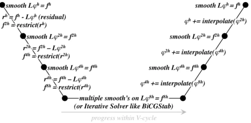
Linear solvers arising from PDEs are ubiquitous in scientific computing. Multigrid is a recursive technique for solving elliptic PDEs in which the solution (or correction for the residual equation) for a large problem is re-cursively approximated by the correction on a smaller (coarsened) problem. This recursion continues until only a trivial problem remains. The resultant coarse grid (or bottom) solve can be computed efficiently. Multigrid solvers iterate on the resultant recursive V-Cycle shown in Figure 1. At each level of the multigrid V-cycle, a number of linear operations are performed including smooth, residual, restriction, and interpolation.

Geometric multigrid is a specialization in which data laid out on a regular grid is used to specialize the implementation of the linear operator (sparse matrices become stencils) as well as the transfer between coarse (φ2h) and fine (φh_{) grid points.}

In this paper, we use miniGMG, a compact, distributed memory bench-mark for solving systems of linear equations using geometric multigrid, as the basis for our experiments [20, 33]. miniGMG discretizes the 3D PDE

Lφ = aαφ−b∇ ·β∇φ = f using a 2nd order, cell-centered, finite volume method on a regular, cartesian grid. For spatially variable coefficientsαand

β, this produces a variable coefficient 7-point stencil.

There are two publicly available distributed memory implementations of miniGMG — one threaded with OpenMP and the other accelerated with

progress within V-cycle

Figure 1: The Multigrid V-cycle for solvingLφh=fh. Note, superscripts denote geomet-ric grid spacings.

CUDA (“miniGMG-cuda”). Each of these versions were heavily optimized by the original developer for their respective targets. In this paper, we use these highly-optimized implementations as a metric against which we measure the performance of our productive and portable, compiler-based solution which takes as input, a single, architecture-agnostic MPI implementation, and pro-duces highly-optimized MPI with OpenMP or MPI with CUDA. Note, for ex-pediency, we leverage miniGMG’s existing OpenMP and CUDA-accelerated MPI routines that effect ghost zone exchanges and apply our technology to the stencils – smooth, residual, restriction, and interpolation.

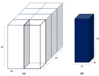
Collection of subdomains owned by an MPI process one subdomain of 643 _elements

Figure 2: Domain decomposition in miniGMG. Each red subdomain represents one “box” for which there are 12 components and 4-8 grid spacings. OpenMP or CUDA parallelism must be applied both within a box and across all boxes owned by the process in question (blue).

3.1. Data Structures in miniGMG

miniGMG solves linear systems on 3D structured (cubical) grids. To affect MPI parallelism, the global 3D domain is decomposed into smaller cubical boxes (Figure 2). As the basis for domain decomposition, each box is self-contained and includes not only all 12 components (coefficients, right-hand side, solution, etc...) for all points in its region of space, but also all local geometric coarsenings of the box’s data. For second-order operators, a one cell deep ghost zone encloses the box. Thus, for boxes that are 643on the finest level with a 1-deep ghost zone, level 0 of the box data structure can be viewed as a 4D data structure grids[12][66][66][66]. As each process contains one or more boxes, each with 4-8 levels, an additional data structure

subdomains[boxes].levels[8] is constructed to index the floating-point

data. miniGMG-cuda uses a similar data structure. However, as it was written in CUDA 4.0 prior to the introduction of CUDA Unified Memory, a shadow copy of this data structure is created on the GPU with a few changes to the pointers within the data structure. For example a pointer on the CPU could point to either data on the CPU or data on the GPU.

For this paper, we modified miniGMG’s data structure slightly. In the original miniGMG benchmark, each subdomain has a list of components, and each component within a subdomain is contiguous in memory. How-ever, the component memory layout is not contiguous across subdomains. miniGMG was modified to allocate each component as a contiguous chunk of memory. This means, that each component in a subdomain is contiguous and components are also contiguous across subdomains.

This data layout allows us to effectively parallelize the computation in-side each box and across boxes. As shown in Listing 1, our input code to CUDA-CHiLL has a four-deep loop nest. The outermost loop iterates through all the boxes in the domain. Furthermore, our arrays (grids) are four-dimensional, reflecting the outermost box loop. To correctly accom-modate four-dimensional array references, the grid creation and allocation routines in miniGMG benchmark had to be modified. Each643 subdomain (box) has a number of associated 663 grids. Thus for the entire domain (2563_{), each grid: phi, beta_i, beta_j, beta_k, rhs, lambda, alpha, is} a list of 663 grids. In the miniGMG benchmark, each 663 grid is allocated a contiguous chunk of memory, but consecutive grids for a component, e.g.,

phi, are not contiguous in memory.

3.2. Operations in miniGMG

There are four basic operations in miniGMG — smooth, residual, restric-tion, and interpolation — all of which are stencil operations on regular grids.

In this paper, we explore two different types of smoothing Gauss-Seidel Red-Black (GSRB) and Jacobi. Whereas Jacobi smoothers simply iterate over all grid points in parallel performing the operationφn+1_=φn_+cD−1_(f−Lφ), GSRB colors the grid cells in a red-black checkerboard in 3D and applies the smootherφ=φ+D−1(f−Lφ)to one color of cell at a time. Although Jacobi is often used for computer science research, GSRB is far more com-mon in scientific computing and much more challenging for compilers. In order to further highlight the value of our autotuning compiler technology, we evaluate performance for two different versions of the linear operatorL. The first is a variable coefficient finite volume operator found in many real-world codes while the second is the ubiquitous 7-point constant coefficient stencil found in many papers.

1 #define PR_SIZE 64

2 #define NUM_BOXS 64

3 void smooth_GSRB(double a, double b, double h, int sweep){

4

5 double _phi[NUM_BOXS][PR_SIZE+2][PR_SIZE + 2][PR_SIZE + 2];

6 double _rhs[NUM_BOXS][PR_SIZE+2][PR_SIZE + 2][PR_SIZE + 2];

7 double _alpha[NUM_BOXS][PR_SIZE+2][PR_SIZE + 2][PR_SIZE + 2];

8 double _beta_i[NUM_BOXS][PR_SIZE+2][PR_SIZE + 2][PR_SIZE + 2];

9 double _beta_j[NUM_BOXS][PR_SIZE+2][PR_SIZE + 2][PR_SIZE + 2];

10 double _beta_k[NUM_BOXS][PR_SIZE+2][PR_SIZE + 2][PR_SIZE + 2];

11 double _lambda[NUM_BOXS][PR_SIZE+2][PR_SIZE + 2][PR_SIZE + 2];

12 double h2inv = 1.0/(h*h);

13 int i,j,k; int box;

14 int color = sweep; double _t;

15

16 for(box=0; box<NUM_BOXS; box++){

17 for(k=1; k<=PR_SIZE; k++){

18 for(j=1; j<=PR_SIZE; j++){

19 for(i=1; i<=PR_SIZE; i++){

20 if(( i+ j + k + (color) ) % 2 == 1 ) {

21 _t = b*h2inv*(

22 + _beta_i[box][k][j][i+1]*( _phi[box][k][j][i+1]-_phi[box][k][j][i ] )

23 - _beta_i[box][k][j][i ]*( _phi[box][k][j][i ]-_phi[box][k][j][i-1] )

24 + _beta_j[box][k][j+1][i]*( _phi[box][k][j+1][i]-_phi[box][k][j ][i] )

25 - _beta_j[box][k][j ][i]*( _phi[box][k][j ][i]-_phi[box][k][j-1][i] )

26 + _beta_k[box][k+1][j][i]*( _phi[box][k+1][j][i]-_phi[box][k ][j][i] )

27 - _beta_k[box][k ][j][i]*( _phi[box][k ][j][i]-_phi[box][k-1][j][i] ));

28 _t = a*_alpha[box][k][j][i]*_phi[box][k][j][i] - _t;

29 _phi[box][k][j][i] = _phi[box][k][j][i]

-30 _lambda[box][k][j][i]*(_t -_rhs[box][k][j][i]);

31 }}}}}

32 }

Listing 1: Input C code for GSRB smooth with 4D arrays

Listing 1 shows the code for the variable coefficient GSRB smoother that is input to CUDA-CHiLL. The arrays defined in the function do not have

assignments as this code is intended to be consumed by CUDA-CHiLL. The code generated by CUDA-CHiLL is post-processed by a python script which replaced these array definitions with appropriate assignment and pointer casting. This is shown in generated code in Listing 6. The GSRB code performs a single sweep (red or black) on all boxes and all matching points in the box. At each point (excluding ghost zones), the variable-coefficient operator is applied to_phiwith the result being stored in_t. Note, although an in-place update would nominally cause a data hazard, the red-black nature of the update ( i+ j + k + (color) ) % 2 eliminates the data hazard by ensuring (aside from the point itself) only “black” data is read on a “red” update. As residual calculations are very similar to Jacobi smoothers, taking the formr =f −Lφ, all 6 combinations of smoother/residual and operator show very similar implementations and challenges.

Listing 2 shows miniGMG’s third major operator, restriction which per-forms the operation u2h = R2_hhuh and is used to create a coarse grid right-hand side from a fine-grid residual. Unlike many conventional stencil oper-ations, the linear operator R2_hh is not square. Rather it must geometrically restrict a fine grid of size N2 to another (disjoint) coarse grid of size (N/2)2 by averaging fine grid cells. Like miniGMG’s smoothers, this routine iter-ates over all boxes, but unlike conventional stencils, the fine grid indices are linearly scaled by 2 from the loop indices creating something akin to a stride two memory access pattern.

1 #define PR_SIZE 64

2 #define NUM_BOXS 64

3 void restriction( int fine_id, int coarse_id, int fine_level){

4 int i,j,k; int box;

5 double _fine[NUM_BOXS][ PR_SIZE + 2][ PR_SIZE + 2][ PR_SIZE + 2];

6 double _coarse[NUM_BOXS][(PR_SIZE/2) + 2][(PR_SIZE/2) + 2][(PR_SIZE/2) + 2];

7 for(box=0; box<NUM_BOXS; box++){

8 for(k=0; k< PR_SIZE/2; k++){

9 for(j=0; j< PR_SIZE/2; j++){

10 for(i=0; i< PR_SIZE/2; i++){

11 _coarse[box][k][j][i] = 0.125 *

12 ( _fine[box][2*k ][2*j ][2*i] + _fine[box][2*k ][2*j ][2*i+1] +

13 _fine[box][2*k ][2*j+1][2*i] + _fine[box][2*k ][2*j+1][2*i+1] +

14 _fine[box][2*k+1][2*j ][2*i] + _fine[box][2*k+1][2*j ][2*i+1] +

15 _fine[box][2*k+1][2*j+1][2*i] + _fine[box][2*k+1][2*j+1][2*i+1]) ;

16 }}}}

17 }

Listing 2: Input C code for restriction.

Listing 3 shows miniGMG’s fourth major operator, interpolation which can be thought of as the inverse of restriction. That is, interpolation, uh =

I₂h_hu2h, maps a coarse grid of size (N/2)3 onto a fine grid of size N3. As it is almost invariably used in the V-Cycle to correct a fine-grid solution, we have merged the increment operation to form uh _{= u}h _+Ih

2hu2h. For

a second-order accurate solver, piecewise constant interpolation will suffice. Here, a coarse grid cell value is used to increment the 8 enclosing fine grid cell values. Once again, the operator presents a challenge to compilers as one must either divide loop indices by two to map to the coarse grid (stride one-half) or scale them by two to map to the fine grid (stride-2). We choose the latter.

1 #define PR_SIZE 64

2 #define NUM_BOXS 64

3 void interpolation( int fine_id, int coarse_id, int fine_level){

4 int i,j,k; int box;

5 double _fine[NUM_BOXS][ PR_SIZE + 2][ PR_SIZE + 2][ PR_SIZE + 2];

6 double _coarse[NUM_BOXS][(PR_SIZE/2) + 2][(PR_SIZE/2) + 2][(PR_SIZE/2) + 2];

7 for(box=0; box<NUM_BOXS box++){

8 for(k=0; k< PR_SIZE/2; k++){

9 for(j=0; j< PR_SIZE/2; j++){

10 for(i=0; i< PR_SIZE/2; i++){

11 _fine[box][2*k ][2*j ][2*i ] += _coarse[box][k][j][i];

12 _fine[box][2*k ][2*j ][2*i+1] += _coarse[box][k][j][i];

13 _fine[box][2*k ][2*j+1][2*i ] += _coarse[box][k][j][i];

14 _fine[box][2*k ][2*j+1][2*i+1] += _coarse[box][k][j][i];

15 _fine[box][2*k+1][2*j ][2*i ] += _coarse[box][k][j][i];

16 _fine[box][2*k+1][2*j ][2*i+1] += _coarse[box][k][j][i];

17 _fine[box][2*k+1][2*j+1][2*i ] += _coarse[box][k][j][i];

18 _fine[box][2*k+1][2*j+1][2*i+1] += _coarse[box][k][j][i];

19 }}}}

20 }

Listing 3: Input C code for interpolation.

4. Code generation with CUDA-CHiLL

The research presented in this paper uses the loop transformation and code generation tool CUDA-CHILL. CUDA-CHiLL is a thin layer built on top of CHILL and extends the code generation capabilities of CHiLL to target GPUs via the CUDA programming model.

4.1. CHiLL Background

CHiLL is a loop transformation and code generation framework with a scripting language interface. CHiLL was designed to support autotuning by allowing sequences of transformations to be composed and applied. CHiLL also exposes parameters of the transformations for autotuning. The input to CHiLL is a source code written in C (or Fortran), and a transformation

script. The script describes the set of transformations to be composed to optimize the provided source [9]. After applying optimizations specified in the script, CHiLL generates optimized C (or Fortran) code. Recently CHiLL has been extended to generate OpenMP code [2].

At the heart of CHiLL is a polyhedral framework that composes com-plex transformation sequences. Internally CHiLL uses Omega+, an enhanced version of Omega [24], and Codegen+ [3]. A polyhedral model represents each statement’s execution in the loop nest as a lattice point in the space constrained by loop bounds, known as the iteration space. Then a loop trans-formation can be simply viewed as a mapping from one iteration space to another. CHiLL manipulates iteration spaces derived from the original pro-gram based on the transformation in the input script and uses a dependence graph as an abstraction to reason about the safety of the transformations under consideration [1]. In CHiLL, iteration spaces are represented as integer sets, and loop transformations are linear mappings applied to these integer sets. Omega+ is used to represent the integer sets as linear mappings, apply the mappings to the integer sets which results in transforming the iteration spaces of the loops, and compute data dependences. CHiLL uses mapping iteration spaces of loop nests to implement a number of well-known loop transformations such as loop tiling, skewing such permutation. Once the transformations have been applied, and iteration spaces have been modified, Codegen+ scans the new iteration spaces to generate code [3]. As mentioned earlier, CHiLL generates C (serial and with OpenMP) and Fortran code.

4.2. CUDA-CHiLL Background

CUDA-CHiLL has a scripting language (Lua programming language) in-terface and uses the loop tiling and iteration space or polyhedral scanning in CHiLL to generate parallel CUDA code.GPUs are a tiled architecture where each streaming multiprocessor (SM) represents a separate tile. Parallel code should be partitioned across SMs so that each thread operates on mostly in-dependent, localized data. This is done by using CUDA-CHiLL’s loop tiling capabilities. Subdividing the iteration space of a loop into blocks or tiles with a fixed maximum size has been widely used when constructing parallel computations [34, 12, 14]. By varying the parameters to the tiling command in the CUDA-CHiLL Lua scripts, the shape and size of the tile in the gen-erated code can be chosen to take advantage of the target parallel hardware and memory architecture.

2D Thread Block 3D Grid of Thread Blocks

TX = 32 TY = 16 BX = 2 B Y = 4 (a) (b)

Figure 3: Organization of CUDA threads into a 3D (2,4,64) grid with 2D (32,16) thread blocks. Each 2D (X,Y) plane in the 3D grid has 8 2D thread blocks of dimension (32,16). Each 2D plane in the 3D grid works on a single subdomain (box) in miniGMG, and there are 64 such planes to process 64 subdomains.

32 16 64 64 64 64 (a) (b)

Figure 4: Illustration of work done by each thread block. Figure (a) shows 8, (32,16) thread blocks working on a643 _{subdomain (box), with each thread computing a column}

of 64 output points. The blue column in figure (b) represents the 32*16*64 = 32,768 output grid points computed by each thread block.

4.3. Parallel Decomposition of GMG

Before discussing how CUDA-CHiLL is used to generate CUDA code for the key operations in miniGMG, we present how the parallelism in the GMG operations – smooth, residual, restriction and interpolation are mapped to GPUs. Code for GPUs has to effectively use the two-level parallelism hier-archy in CUDA, which is expressed in terms of a grid of thread blocks. As illustrated in Figure 3, GPU kernels are implemented in miniGMG using a 3D grid of 2D thread blocks.

The rationale behind 2D thread blocks is that the 2D blocks are used to tile the iand j dimensions of each box (i is the dimension of unit stride), and the k dimension is not tiled (k dimension has the largest stride). Not tiling the dimension of maximum stride is known as Rivera Tiling [26], and has been shown to improve the performance of 3D scientific codes. A di-mension of the 3D grid is used to map to each box or subdomain, the other two dimensions of the 3D grid control the number of thread blocks working on each box. Using a 3D grid allows exploring a larger space of parallel decompositions, as the 3D grid can easily be reduced to a 2D grid by setting one of the two dimensions of the grid to unity (the third dimension of the grid is always set to the number of boxes).

The 3D grid of CUDA thread blocks is of dimension {BX,BY,BZ}. Each 2D CUDA thread block is of dimension{TX,TY}. To make the explanation concrete, we use an example thread decomposition of a 2563 domain which is split into a list of 64×643 subdomains. The 3D CUDA grid of thread blocks has dimensions {BX=2, BY= 4, BZ=64 (number of boxes)}. Each 2D thread block in this grid has dimensions {TX=32, TY= 16}. The BZ dimension of the grid maps to boxes (subdomains), each plane {BX=2, BY= 4} of thread blocks in the grids is assigned to a single643 box or subdomain. Thus, there are eight thread blocks working inside a box, and 64 {BZ=64} planes of 2D thread blocks, with each plane working on box. This block and grid arrangement is shown in Figure 3.

Figure 4 illustrates how the 2D CUDA thread blocks process each 643

box. The thread blocks encompass theij-planes of the box, but not thek -dimension. In terms of memory layout, iis the fastest-changing dimension andkthe slowest. As mentioned earlier, in this decomposition, the dimension

kis not tiled. Thus, each CUDA thread computes 64 output grid points (in the k dimension), and each thread block computes 32(TX)*16(TY)*64 = 32,768 output points. The optimized smooth in miniGMG uses a 3D grid of dimension {BX=2, BY= 16, BZ=64}, and 2D thread blocks {TX=32, TY= 4} [32].

4.4. CUDA-CHiLL Scripts for miniGMG Operators

The parallelization strategy described in the previous section is used by expert programmers and also used to generate CUDA code with CUDA-CHiLL. CUDA-CHiLL is used to tile the input four-deep loop nests in the input sequential code for smooths, residuals, restriction and interpolation to create two more loop levels. To create a 3D grid with 2D thread blocks, three out of these six loops are then mapped to blocks in the 3D grid, and two loop levels are mapped to threads in a 2D block.

Listing 4 illustrates the script that drives CUDA-CHiLL to generate a CUDA kernel for GSRB. The tile commands in line 12 of the script tile the loops in the input loop nest. The first argument to tile is the statement number (CUDA-CHiLL treats the entire loop body as a single statement). The next argument is the set of input loops to be tiled. This is followed by the tile sizes, the names of the tile controlling loops, and the final order of resulting tiled and tile controlling loops.

Listing 5 shows the structure of the loop nest after tiling. The tile con-trolling loop bb and kk have a single iteration and are not generated by CUDA-CHiLL. This effectively means that loopsbox, andk have not been tiled. The cudaize command in line 17 of Listing 4 then marks the can-didate loops for block and thread dimensions. Loops box, jj and ii are marked as dimensions of the 3D grid. Loopsi, andj are marked as the di-mensions of the 2D thread blocks. During CUDA code generation the loops marked as dimensions for grids and blocks are removed, and array references to those loop indices are replaced with block indices (bx, by, bz) or thread indices (tx, ty). 1 init("gsrb.cu", "gsrb",0,0) 2 dofile("cudaize.lua") 3 --tile sizes 4 N=64 5 TI=32 6 TJ=16 7 TK=64 8 TZ=64

9 --end tile sizes

10 tile_by_index(0,

11 {"box","k","j", "i"},{TZ,TK, TJ, TI},

12 {l1_control="bb", l2_control="kk", l3_control="jj", l4_control="ii"}, 13 {"bb","box","kk","k","jj","j","ii","i"})

14

15 cudaize(0, "kernel_GPU",{},

16 {block={"ii","jj","box"}, 17 thread={"i","j"}},{})

4.5. Space of Generated Code Variants

Simple autotuners were written in Python to generate CUDA-CHiLL scripts to generate CUDA variants of smooths, residuals, restriction and interpolations. In this discussion we will focus on variants for the GSRB smoother, variants for other operations were generated similarly. The gen-erated code variants were then run in the miniGMG framework.

Code variants were created by varying the dimensions of the 2D thread block. If the size of a thread block is <TX,TY>, the dimension of the 3D grid for the finest grids is <64/TX, 64/TY, 64>, where each subdomain is

643. For the finest grids the variants were created by varying TX from 8 to 64, and TY from 4 to 64 such that TX*TY is at least 32 (warp size), and TX*TY≤1024 (maximum number of threads per block).

Code variants for the other operators in miniGMG and for other levels of the V-cycle (from 323 _{down to 4}3_{) was generated using CUDA-CHiLL} scripts generated by python scripts. The maximum size of any dimension of the 2D thread blocks were the size of the box/grid at the level of the V-cycle for smooth and residual operators. For restriction and interpolation, the maximum size of any dimension of the thread block was the size of the smaller/coarser grid.

1 // ~cuda~ preferredIdx: bz

2 for(box = 0; box <= 63; box++) {

3 // ~cuda~ preferredIdx: k 4 for(k = 1; k <= 64; k++) { 5 // ~cuda~ preferredIdx: by 6 for(jj = 0; jj <= 3; jj++) { 7 // ~cuda~ preferredIdx: ty 8 for(j = 0; j <= 15; j++) {

9 // ~cuda~ threadLoop preferredIdx: bx

10 for(ii = 0; ii <= 1; ii++) {

11 // ~cuda~ preferredIdx: tx

12 for(i = intMod(-j-k-color-1,2); i <= 31; i += 2) {

13 S0();

14 }}}}}}

1 __global__ void __smooth_GSRB( double a, double b, double h, int sweep){ 2

3 double _* phi = gpu_subdomains[0].levels[level].grids[ phi_id];

4 double * rhs = gpu_subdomains[0].levels[level].grids[ rhs_id];

5 double _* alpha = gpu_subdomains[0].levels[level].grids[ __alpha];

6 double _* beta_i = gpu_subdomains[0].levels[level].grids[__beta_i];

7 double _* beta_j = gpu_subdomains[0].levels[level].grids[__beta_j];

8 double _* beta_k = gpu_subdomains[0].levels[level].grids[__beta_k];

9 double * lambda = gpu_subdomains[0].levels[level].grids[__lambda];

10 double _{(*_phi)[PR_SIZE+2][PR_SIZE + 2][PR_SIZE + 2];}

11 double _{(*_rhs)[PR_SIZE+2][PR_SIZE + 2][PR_SIZE + 2];}

12 double _{(*_alpha)[PR_SIZE+2][PR_SIZE + 2][PR_SIZE + 2];}

13 double _{(*_beta_i)[PR_SIZE+2][PR_SIZE + 2][PR_SIZE + 2];}

14 double (*_beta_j)[PR_SIZE+2][PR_SIZE + 2][PR_SIZE + 2];

15 double (*_beta_k)[PR_SIZE+2][PR_SIZE + 2][PR_SIZE + 2];

16 double _{(*_lambda)[PR_SIZE+2][PR_SIZE + 2][PR_SIZE + 2];}

17 _phi = ((double _{(*)[PR_SIZE+2][PR_SIZE + 2][PR_SIZE + 2])phi);}

18 _rhs = ((double _{(*)[PR_SIZE+2][PR_SIZE + 2][PR_SIZE + 2])rhs);}

19 _alpha = ((double (*)[PR_SIZE+2][PR_SIZE + 2][PR_SIZE + 2])alpha);

20 _beta_i = ((double (*)[PR_SIZE+2][PR_SIZE + 2][PR_SIZE + 2])beta_i);

21 _beta_j = ((double _{(*)[PR_SIZE+2][PR_SIZE + 2][PR_SIZE + 2])beta_j);}

22 _beta_k = ((double _{(*)[PR_SIZE+2][PR_SIZE + 2][PR_SIZE + 2])beta_k);}

23 _lambda = ((double _{(*)[PR_SIZE+2][PR_SIZE + 2][PR_SIZE + 2])lambda);}

24 int color = sweep; double h2inv = 1.0/(h*h);

25 int k; int by; by = blockIdx.y;

26 int bz; bz = blockIdx.z; int tx; tx = threadIdx.x; int ty; ty = threadIdx.y;

27 28 for (k = 1; k <= 64; k += 1) 29 if ((tx - (-ty - k - color - 1)) % 2 == 0) { 30 _t = b * h2inv * (_beta_i[bz][k][ty + 16 * by + 1][tx + 1 + 1] * 31 (_phi[bz][k][ty + 16 * by + 1][tx + 1 + 1] 32 -_phi[bz][k][ty + 16 * by + 1][tx + 1]) 33 - _beta_i[bz][k][ty + 16 * by + 1][tx + 1] 34 * (_phi[bz][k][ty + 16 * by + 1][tx + 1] 35 - _phi[bz][k][ty + 16 * by + 1][tx + 1 - 1]) 36 + _beta_j[bz][k][ty + 16 * by + 1 + 1][tx + 1] 37 *(_phi[bz][k][ty + 16 * by + 1 + 1][tx + 1] 38 - _phi[bz][k][ty + 16 * by + 1][tx + 1]) 39 - _beta_j[bz][k][ty + 16 * by + 1][tx + 1] 40 _{* _phi[bz][k][ty + 16 * by + 1][tx + 1]} 41 - _phi[bz][k][ty + 16 * by + 1 - 1][tx + 1]) 42 + _beta_k[bz][k + 1][ty + 16 * by + 1][tx + 1] 43 *(_phi[bz][k + 1][ty + 16 * by + 1][tx + 1] 44 - _phi[bz][k][ty + 16 * by + 1][tx + 1]) 45 - _beta_k[bz][k][ty + 16 * by + 1][tx + 1] 46 * (_phi[bz][k][ty + 16 * by + 1][tx + 1] 47 - _phi[bz][k - 1][ty + 16 * by + 1][tx + 1])); 48 _t = a * _alpha[bz][k][ty + 16 * by + 1][tx + 1] 49 * _phi[bz][k][ty + 16 * by + 1][tx + 1] - _t; 50 _phi[bz][k][ty + 16 * by + 1][tx + 1] = _phi[bz][k][ty + 16 * by + 1][tx + 1] 51 - _lambda[bz][k][ty + 16 * by + 1][tx + 1] 52 * (_t - _rhs[bz][k][ty + 16 * by + 1][tx + 1]);} 53 }

Listing 6: Generated CUDA code for GSRB smooth. The generated code is for 2D thread blocks (TX=64, TY=16) and 3D grid (BX=1, BY=4,BZ=64).

4.6. Extensions to CUDA-CHiLL Code Generation

CUDA-CHiLL was built on top of CHiLL to generate CUDA code. It uses CHiLL to apply loop transformations (such as tiling), and then leverages the code generation capabilities of Codegen+. Once Codegen+ scans the polyhedra representing the iteration space of the loop nest, it creates an intermediate representation or abstract syntax tree (AST) representation of the output code. CUDA-CHiLL works on this AST and modifies it to generate CUDA code by mapping loops to thread and block indices. In the current implementation, only normalized loops can be mapped to a thread block index, which means candidate loops must have a lower bound of 0, and a unit stride.

The complex if-condition involving a modulo operation in GSRB presents a code generation challenge to CUDA-CHiLL. This is because the if-condition which guards the statement in GSRB gets fused into the innermost for-loop once Codegen+ creates an output. This can be seen in the innermost loop in Listing 5, which has a complex conditional with a modulo condition as a lower bound, and the loop has strided access. Thus, the loop is not normalized, and cannot be mapped to a thread or block index. To remedy the situation, CUDA-CHiLL was extended to handle such strided loops. The modulo condition will be removed from the lower bounds of the loop, and the loop stride will be reduced to one. The if-condition with the modulo would be pushed back into the loop body by creating a new AST node for the if-condition and wrapping the statement in the loop inside the AST node. This change checks to see if the stride of the loop matches the right hand side of the modulo in the if-condition. The output CUDA code in Listing 6 illustrates how the if-condition gets pushed back into the body of the loop.

The CUDA variants generated by CUDA-CHiLL are post-processed by a Python script to make the code generated usable in the miniGMG bench-mark. The code generated by CUDA-CHiLL has the array declaration with-out assignments as shown in Listing 1. The post-processing python script replaces these array declaration with declarations and assignments shown in Listing 6.

5. Performance Portability Results 5.1. Experimental Setup

In this paper, we use both CPU-based and GPU-accelerated systems to demonstrate CHiLL affords performance portability across diverse archi-tectures. The relevant performance characteristics of the two systems are presented in Table 1.

Edison Titan

Processor Intel Ivy Bridge AMD Interlagos NVIDIA Kepler

Clock 2.4GHz 2.2GHz 0.733GHz

NUMA×Cores 2×12 2×8 1×14

DP GFlop/s per node 461 140 1314

STREAM per node 97 31 1603

Data caches per core 32+256KB 16+2048KB1 64+48KB2

Last-level cache per NUMA 30MB 8MB 1.5MB

System and System Software

Nodes 5,576 18,688

Interconnect Dragonfly 3D torus + local PCIe

Complier Intel 16 Intel 15 nvcc 7.0 Table 1: Systems used in this study.1Pairs of cores share a L2 cache and FPU.2L1 data cache + read-only (texture) cache. 3Obtained via the Empirical Roofline Toolkit [16]

Edison is a Cray XC30 located at NERSC [21] and accepted in 2013. Each node contains two high-performance, massively out-of-order, 12-core Ivy Bridge processors each capable of 230 GFlop/s and 50 GB/s of DRAM bandwidth. Nodes are interconnected with a high-performance, low radix Aries dragonfly network designed for scalability.

In contrast to Edison’s conventional and homogeneous CPU architecture, Titan is a GPU-accelerated Cray XK7 [23] installed in 2012. Each of Titan’s 18,688 nodes contain two 8-core CPU chips and one PCIe-attached NVIDIA Kepler GPU. Although the CPUs provide a moderate 140 GFlops/s and 31 GB/s of bandwidth, the bulk of the node’s performance comes from the GPU which provides 1.3 TFlop/s of performance and 160 GB/s of bandwidth to local memory. As GPU caches are relatively small and difficult to exploit, we expect tuning for locality to play a larger role on the GPU. Titan’s nodes are interconnected using Cray’s Gemini 3D torus. Compared to the newer Dragonfly, a 3D torus will likely show limited scalability. Note, for codes amenable and optimized for on-device data locality, the limited PCIe bandwidth will not substantially impede performance.

In all our experiments, we use a per-node problem size of 2563 decom-posed into 643 boxes. We run one process per NUMA node. Thus on Edison and Titan(CPU-only), each process receives 32×643 boxes while each Titan GPU receives 64×643. In order to ensure consistent algorithmic comparison, no communication-avoiding optimizations were employed on either platform. We use 4-pre and 4-post smooths per level and a total of 10 V-Cycles. For a coarse grid solver, we use 48 smooths for single node experiments, and BiCGStab for multinode experiments.

5.2. Performance Bounds

In order to qualify our results, we can create performance bounds for the two stencil discretizations used in this paper. The first is the general variable coefficient implementation Lφ = aαφ −b∇ ·β∇φ where α is a cell-centered coefficient, there are three face-centeredβ coefficients, and two scalar coefficients a and b. The second is a specialized constant-coefficient operatorLφ=aφ−b∇2_{φderived by settingα ==β == 1for all points in} space.

In both cases, the discretized operators are 3D 7-point stencils in φ. Although they both must read 7 values of u from memory, the cache, with proper blocking, will filter all but one reference from reaching main memory. Similarly, although the variable coefficient operator must read 6 values of

β (one per cell face), all but three are filtered by the cache. As a result, the variable coefficient operator will read on average at least 5 doubles from memory per stencil while the constant coefficient operator only one.

In the optimized miniGMG solvers, the linear operator Lφ rarely ap-pears in isolation. Rather, the bulk of the applications of the stencil appear in the smoothers. In this paper, we examined CHiLL’s ability to optimize two different stencils — Red-Black Gauss Seidel (GSRB) and Jacobi. Al-though both stencils take the formφn+1 _=φn_+cD−1_{(f−Lφ), their iteration} spaces are somewhat different with Red-Black striding through memory and aliasing φn+1 to φn (in-place updates). Interestingly, for conventional data layouts ofφandα, this striding through memory does not affect data move-ment, but only the requisite number of floating-point operations. Assuming a write-allocate cache architecture (perhaps untrue on GPUs), we can cal-culate the compulsory data movement as 64, 72, 32, and 40 bytes per stencil for GSRB variable coefficient, Jacobi variable coefficient, GSRB constant co-efficient, Jacobi constant coefficient respectively. In terms of floating-point operations, these smoothers require about 12, 24, 6, and 13 flops per cell (not stencil) respectively. With arithmetic intensities less than 0.33, performance is expected to be memory-bound and we can bound run time based on the data movements from this section coupled with the stream bandwidths in Table 1. As such, we can easily construct a Roofline performance bound for each machine for each benchmark [31].

5.3. Performance Portability Across Diverse Node Architectures

In order to demonstrate performance portability, we run the miniGMG solver on Edison, Titan(CPU-only), and Titan(GPU-only) using CHiLL to generate the key computational kernels discussed above.

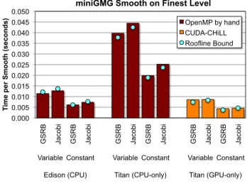
Figure 5 shows the time spent per fine grid smooth (a 2563 domain per node decomposed into 64×643 boxes on the finest multigrid level) on our three machines as a function of smoother (GSRB vs. Jacobi) and discretiza-tion of the Laplacian (variable vs. constant coefficient). In all cases, we use a single compute node with 2 MPI processes per node on the CPU-only results (OpenMP auto-generated/autotuned with CHiLL) and one for the GPU-only results (CUDA auto-generated/autotuned with CUDA-CHiLL). To provide a performance reference across widely ranging architectural ca-pabilities and differing stencils, we use a Roofline performance bound (blue circles). 0.000 0.005 0.010 0.015 0.020 0.025 0.030 0.035 0.040 0.045 0.050 G SR B Ja co bi G SR B Ja co bi G SR B Ja co bi G SR B Ja co bi G SR B Ja co bi G SR B Ja co bi

Variable Constant Variable Constant Variable Constant

Edison (CPU) Titan (CPU-only) Titan (GPU-only)

T im e p er Sm o o th (s ec o n d s)

miniGMG Smooth on Finest Level OpenMP by hand CUDA-CHiLL Roofline Bound

Figure 5: Performance of CUDA-CHiLL generated smooths on the finest level(643boxes). The GPU code is generated by CUDA-CHiLL. The code for CPUs are handwritten code from the miniGMG benchmark. The CPU code uses MPI+OpenMP for parallelization, but does not used optimizations such as wavefronts or explicit SIMDization.

We observe that CHiLL, with auto-generated/tuned OpenMP and/or CUDA, delivers exceptional performance across all machines and stencils. On the GPU, CUDA-CHiLL exploits 85% of the machine’s potential 160 GB/s of bandwidth while on Edison, CHiLL can actually exceed the Roofline bound. This is not to say it exceeds the DRAM pin bandwidth, but rather STREAM Triad does not fully exploit the DRAM bandwidth of the Ivy Bridge processor. Generally, speaking, GPUs show substantial performance boosts over CPUs on the same machine (Titan’s GPUs vs. Titan’s CPUs). However, more recent CPUs (Edison) have substantially narrowed the per-formance gap.

5.4. Performance Portability Across Problem Size

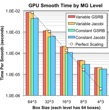
Multigrid’s performance is premised on the theory that time is directly proportional to problem size. With exponentially smaller boxes in the V-Cycle, one must realize exponentially lower run time per level in order for O(N) computational complexity to turn into O(N) run time. Figure 6 shows the time per smooth by level in the CUDA-CHiLL autotuned miniGMG-cuda. For visualization purposes, we add a perfect scaling reference line based on fine-grid variable coefficient GSRB ignoring ghost zones. Generally speaking, we see no performance differences between smoother or discretiza-tion indicating that CUDA-CHiLL has delivered consistent performance on each level independent of the underlying stencil. Although the first three levels generally track the perfect scaling trend line, the coarsest two levels (64×83 and 64×43) quickly depart and saturate at about 20us — a time roughly equal to the CUDA kernel launch time on PCIe attached GPUs. Es-sentially, the time to launch work on the GPU swamps any execution time on the GPU and thus time saturates. It should be noted that NVIDIA avoids this issues in their HPGMG-CUDA implementation by running the coarse grid operations on the CPU using OpenMP [11]. Future work will move towards unifying CHiLL and CUDA-CHiLL so that it can generate both CPU(OpenMP) and GPU(CUDA) code and select the appropriate variant at run time.

At each level of the multigrid V-Cycle, CUDA-CHiLL autotuned its gen-erated kernels to decide the appropriate thread block size. Smaller thread blocks reduce cache and register pressure and tend to increase occupancy. Unfortunately, progressively smaller thread blocks must load disproportion-ally more inter thread block ghost zone data and thus can increase data move-ment and actually increase total cache pressure per SM. The upper bound on thread block size is actually dictated by CUDA itself at 1K threads. Note, for this problem, there are always 64 boxes per level per node. As such, kernels aways have a z-dimension of 64 and x- and y-dimensions equal to 256 divided by the thread block x-and y-dimensions. Moreover, thread blocks are 2D and sweep through all elements in the z dimension within a box.

Table 2 shows the best performing thread block dimensions as determined by CUDA-CHiLL’s autotuning. Generally speaking, we observe that the best configurations did not tile any box 643 or smaller in the x-dimension. Inter-estingly, constant coefficient discretizations, which nominally have reduced cache and register pressure, preferred smaller y-dimensions, while GSRB further reduced the y-dimension. The ability for CUDA-CHiLL to indepen-dently tune the thread block size not only for each machine, but for each operator and each problem size, greatly facilitates performance portability.

1.0E-06 1.0E-05 1.0E-04 1.0E-03 1.0E-02 64^3 32^3 16^3 8^3 4^3 T im e Pe r Sm o o th (s ec o n d s)

Box Size (each level has 64 boxes) GPU Smooth Time by MG Level

Variable GSRB Variable Jacobi Constant GSRB Constant Jacobi Perfect Scaling

Figure 6: Performance of CUDA-CHiLL generated smooths at each level of the V-cycle. Observe near linear performance until run time falls below the CUDA kernel launch time.

Smooth 64×643 64×323 64×163 64×83 64×43

VC GSRB <64,8,1> <32,8,1> <16,4,1> <8,8,1> <4,4,1> VC Jacobi <64,16,1> <32,4,1> <16,16,1> <8,8,1> <4,4,1> CC GSRB <64,4,1> <32,8,1> <16,4,1> <8,4,1> <4,4,1> CC Jacobi <64,8,1> <32,4,1> <16,16,1> <8,8,1> <4,4,1>

Table 2: Best-performing thread block configurations for generated smooths at different levels of the V-cycle. CUDA-CHiLL’s autotuning approach found the best performing implementation on each level for each smoother for each stencil.

5.5. Interoperability with MPI and Scalability

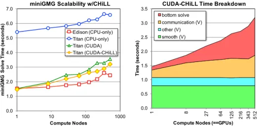
In order to demonstrate that CHiLL and CUDA-CHiLL are interopera-ble with MPI without performance penalties, we conducted a series of ex-periments on Edison(CPU-only), Titan(CPU-only), and Titan(GPU-only) in which we weak scale with the same 2563 problem per node but with a BiCGStab bottom solver. Figure 7(left) shows performance generally scales well on all platforms with the Edison’s Aries Dragonfly generally delivering

superior scalability. Performance at 8 nodes clearly shows the moderate per-formance penalties associated with PCIe-attached GPUs. Generally speak-ing, CUDA-CHiLL delivers both performance and scalability comparable to the hand-optimized miniGMG-cuda — a testament to the productivity advantage of auto-generating and autotuning CUDA kernels rather than im-plementing/optimizing them by hand.

Careful observation shows that while the both GPU implementations do not scale as well as the CPU version. This is a confluence of several factors. First, Figure 7(right) shows “smooth” and “other” (residual, interpolation, restriction, etc...) times remain constant across scales while the bottom solve and communication time rapidly increase. Second, as discussed ear-lier, GPUs deliver poor performance on the very coarse grids associated with a bottom solver. Third, ghost zone exchanges on the GPU now re-quire transiting PCIe (note, CUDA direct implementations generally further underperformed). 0.0 1.0 2.0 3.0 4.0 5.0 6.0 7.0 1 10 100 1000 mi n iG M G S o lv e T ime ( s e c o n d s ) Compute Nodes

miniGMG Scalability w/CHiLL

Edison (CPU-only) Titan (CPU-only) Titan (CUDA) Titan (CUDA-CHiLL) 0.0 0.5 1.0 1.5 2.0 2.5 3.0 3.5 1 8 _{27 64} 125 216 343 512 Ti m e ( s e c onds )

Compute Nodes (==GPUs)

CUDA-CHiLL Time Breakdown

bottom solve communication (V) other (V) smooth (V)

Figure 7: (left) Weak scaling of miniGMG-cuda with kernels auto-generated/tuned with CUDA-CHiLL running on Titan’s GPUs compared to the hand-optimized miniGMG-cuda and miniGMG. (right) breakdown of CUDA-CHiLL time on Titan showing the lack of scalability is an artifact of the BiCGStab algorithm and communication. CUDA-CHiLL does not impede scalability.

5.6. Insulating Programmers from Changes in Underlying Compilers

The idea that optimization for a processor today will show benefits on that same processor tomorrow has been ingrained in programmers. miniGMG-cuda was written in 2012-13 in CUDA 4 and initially optimized for Fermi and

subsequently the Kepler GPUs in Titan. Early evaluations on Titan showed substantial manual optimization including placing certain data structures and temporary buffers in shared memory and even restructuring the tiling into non-rectangular tiles (flatten the i-j iteration space and strip mine) in order to ensure aligned access and minimal load imbalance within a thread blocks (in shared memory implementations, threads on the boarder of a thread block have the additional task of loading the implicit ghost zone into shared memory) was required to maximize performance. As such, it was extremely unexpected that in 2016 CUDA-CHiLL substantially out-performed the hand-optimized miniGMG-cuda. As of mid 2016, multiple versions of CUDA were available on Titan ranging from the CUDA 5.0 to CUDA 7.5. To that end, we decided to evaluate miniGMG-cuda and CUDA-CHiLL performance as a function of CUDA compiler version. Figure 8 shows the surprising result that while progressive hand optimization had a gener-ally positive benefit in CUDA 5.0, it had a substantigener-ally negative benefit in CUDA 7.0 resulting in performance that was not only 14% slower than a straightforward tiled implementation, but was 23% slower with CUDA 7.0 than with CUDA 5.0. Conversely, CUDA-CHiLL delivered consistent perfor-mance across implementations simply choosing different code variants and tilings. With a richer set of optimizations, CUDA-CHiLL still would se-lect the best performing implementation for the machine and compiler on hand. The value of CUDA-CHiLL to shield programmers from wasting time optimizing for artifacts in today’s compilers that will be rectified in the fu-ture greatly enhances its ability to deliver enduring performance across both compiler versions and multiple platforms.

6. Conclusions and Future Work

For the last decade, performance portability across CPUs and GPUs has remained elusive as GPUs have required architecture-specific programming models like CUDA, OpenCL, and OpenACC. Although there is extensive optimization of stencil codes for GPUs, efficient geometric multigrid linear solvers demand stencil functions deliver performance for a range of config-urations within the same executable. In this paper we demonstrate that the CHiLL and CUDA-CHiLL autotuning compiler frameworks can auto-matically thread (via OpenMP) or accelerate (via CUDA) the sequential stencil functional descriptions within the miniGMG benchmark. We show that it can attain performance near the Roofline bound for a variety of smoothers and stencil discretizations across a variety of CPU- and GPU-accelerated platforms. With CHiLL’s autotuning capabilities applied across

0.00 0.10 0.20 0.30 0.40 0.50 0.60 0.70 0.80 0.90 1.00 2D tiling, reg pipeline shared memory fuse ij & vectorize autotuned

Hand-Optimized CUDA CUDA-CHiLL Sm o o th T im e (s ec o n d s)

Performance vs. CUDA Version CUDA 5.0 CUDA 7.0

Figure 8: miniGMG-cuda smooth time as a function of both implementation and compiler. Observe that CUDA-CHiLL delivered consistent performance while the best performing hand-optimized implementation compiled with CUDA 5.0 was the worst performing im-plementation with CUDA 7.0.

all-levels within the multigrid V-Cycle we show that a CUDA-CHiLL gen-erated implementation can deliver performance equal to or exceeding the hand-optimized miniGMG-cuda through 512 nodes of the Titan supercom-puter. Although miniGMG’s performance was dominated by operations on the finest few levels of the multigrid V-Cycle, at larger concurrencies, more efficient multigrid algorithms demand high performance on the smaller coarse grids. Unfortunately, we showed that such small problems run inefficiently on PCIe-attached GPUs. To that end, future work will investigate generat-ing both CPU and GPU code and selectgenerat-ing the appropriate version at run time. Finally, a number of GPU-optimized stencil implementations leverage a “register pipeline” in which data is kept and shuffled in the very large reg-ister file rather than the relatively small caches. Although CUDA-CHiLL does not currently implement this optimization, we will investigate its im-plementation in order to reduce cache pressure and fully leverage the GPU architecture. Furthermore we would like to continue working on CUDA-CHiLL to move beyond mini-apps to target larger structured grid codes,

and also look at code-generation techniques for unstructured codes while still using the CHiLL and CUDA-CHiLL compiler framework.

Acknowledgments

This research used resources in Lawrence Berkeley National Laboratory and the National Energy Research Scientific Computing Center, which are supported by the U.S. Department of Energy Office of Science’s Advanced Scientific Computing Research program under contract number DE-AC02-05CH11231. This research used resources of the Oak Ridge Leadership Facil-ity at the Oak Ridge National Laboratory, which is supported by the Office of Science of the U.S. Department of Energy under Contract No. DE-AC05-00OR22725. This material is based upon work supported by the Advanced Scientific Computing Research Program in the U.S. Department of Energy, Office of Science, under Award Number DE-AC02-05CH11231.

References

[1] Randy Allen and Ken Kennedy. Optimizing Compilers for Modern Architec-tures: A Dependence-based Approach. Morgan Kauffman, 2002.

[2] Protonu Basu, Mary W. Hall, Samuel Williams, Brian van Straalen, Leonid Oliker, and Phillip Colella. Compiler-directed transformation for higher-order stencils. InProc. IEEE International Parallel and Distributed Processing Sym-posium (IPDPS), 2015.

[3] Chun Chen. Polyhedra scanning revisited. InProc. ACM SIGPLAN conference on Programming Language Design and Implementation (PLDI), 2012. [4] Chun Chen, Jacqueline Chame, and Mary Hall. CHiLL: A framework for

com-posing high-level loop transformations. Technical Report 08-897, University of Southern California, Jun 2008.

[5] M. Christen, O. Schenk, and H. Burkhart. Patus: A code generation and autotuning framework for parallel iterative stencil computations on modern microarchitectures. InProc. IEEE International Parallel and Distributed Pro-cessing Symposium (IPDPS), 2011.

[6] Kaushik Datta, Shoaib Kamil, Samuel Williams, Leonid Oliker, John Shalf, and Katherine Yelick. Optimization and performance modeling of stencil com-putations on modern microprocessors. SIAM Review, 51(1):129–159, 2009. [7] M. Frigo and V. Strumpen. Evaluation of based superscalar and

cache-less vector architectures for scientific computations. In Proc. ACM Interna-tional Conference on Supercomputing (ICS), 2005.

[8] P. Ghysels, P. Kłosiewicz, and W. Vanroose. Improving the arithmetic intensity of multigrid with the help of polynomial smoothers. Numerical Linear Algebra with Applications, 19(2):253–267, 2012.

[9] Mary W. Hall, Jacqueline Chame, Chun Chen, Jaewook Shin, Gabe Rudy, and Malik Murtaza Khan. Loop transformation recipes for code generation and auto-tuning. In Proc. International Workshop on Languages and Compilers for Parallel Computing (LCPC), Oct 2009.

[10] Justin Holewinski, Louis-Noël Pouchet, and P. Sadayappan. High-performance code generation for stencil computations on gpu architectures. InProc. ACM international conference on Supercomputing (ICS), 2012.

[11] https://bitbucket.org/nsakharnykh/hpgmg-cuda.

[12] F. Irigoin and R. Triolet. Supernode partitioning. InProc. ACM SIGPLAN-SIGACT Symposium on Principles of Programming Languages (POPL), 1988. [13] S. Kamil, C. Chan, L. Oliker, J. Shalf, and S. Williams. An auto-tuning frame-work for parallel multicore stencil computations. InProc. Parallel Distributed Processing (IPDPS), 2010 IEEE International Symposium on, 2010.

[14] Ken Kennedy and Kathryn S. McKinley. Optimizing for parallelism and data locality. InProc. International Conference on Supercomputing (ICS), 1992. [15] Malik Khan, Protonu Basu, Gabe Rudy, Mary Hall, Chun Chen, and

Jacque-line Chame. A script-based autotuning compiler system to generate high-performance cuda code. ACM Trans. Archit. Code Optim., 9(4):31:1–31:25, January 2013.

[16] Terry Ligocki. Roofline toolkit.

[17] Naoya Maruyama and Takayuki Aoki. Optimizing Stencil Computations for NVIDIA Kepler GPUs. InProc. International Workshop on High-Performance Stencil Computations, 2014.

[18] J. McCalpin and D. Wonnacott. Time skewing: A value-based approach to optimizing for memory locality. Technical Report DCS-TR-379, Department of Computer Science, Rutgers University, 1999.

[19] Paulius Micikevicius. 3D finite difference computation on GPUs using CUDA. In Proc. Workshop on General Purpose Processing on Graphics Processing Units, 2009.

[20] miniGMG compact benchmark. http://crd.lbl.gov/departments/

[21] National Energy Research Scientific Computing Center (NERSC). Edi-son website. [Online], Available: http://www.nersc.gov/users/

computational-systems/edison.

[22] Anthony Nguyen, Nadathur Satish, Jatin Chhugani, Changkyu Kim, and Pradeep Dubey. 3.5-D blocking optimization for stencil computations on mod-ern CPUs and GPUs. InProc. ACM/IEEE International Conference for High Performance Computing, Networking, Storage and Analysis (SC), 2010. [23] Oak Ridge Leadership Computing Facility (OLCF). Titan website. [Online],

Available: https://www.olcf.ornl.gov/support/system-user-guides/

titan-user-guide.

[24] William Pugh. The omega test: A fast and practical integer programming algorithm for dependence analysis. In Proc. ACM/IEEE Conference on Su-percomputing (SC), 1991.

[25] Jonathan Ragan-Kelley, Connelly Barnes, Andrew Adams, Sylvain Paris, Frédo Durand, and Saman Amarasinghe. Halide: A language and compiler for optimizing parallelism, locality, and recomputation in image processing pipelines. In Proc. ACM SIGPLAN Conference on Programming Language Design and Implementation (PLDI), 2013.

[26] G. Rivera and C. Tseng. Tiling optimizations for 3D scientific computations. In Proc. International Conference for High Performance Computing, Networking, Storage and Analysis (SC), 2000.

[27] Y. Song and Z. Li. New tiling techniques to improve cache temporal locality. InProc. ACM SIGPLAN Conference on Programming Language Design and Implementation (PLDI), 1999.

[28] Didem Unat, Xing Cai, and Scott B. Baden. Mint: Realizing cuda performance in 3d stencil methods with annotated c. InProc. International Conference on Supercomputing (ICS), 2011.

[29] Gerhard Wellein, Georg Hager, Thomas Zeiser, Markus Wittmann, and Holger Fehske. Efficient temporal blocking for stencil computations by multicore-aware wavefront parallelization. In Proc. International Computer Software and Applications Conference, 2009.

[30] S. Williams, J. Shalf, L. Oliker, S. Kamil, P. Husbands, and K. Yelick. The potential of the Cell processor for scientific computing. In Proc. Conference on Computing Frontiers, 2006.

[31] S. Williams, A. Watterman, and D. Patterson. Roofline: An insightful visual performance model for floating-point programs and multicore architectures. Communications of the ACM, April 2009.

[32] Samuel Williams, Dhiraj D. Kalamkar, Amik Singh, Anand M. Deshpande, Brian Van Straalen, Mikhail Smelyanskiy, Ann Almgren, Pradeep Dubey, John Shalf, and Leonid Oliker. Optimization of geometric multigrid for emerging multi- and manycore processors. Technical Report 6676E, Lawrence Berkeley National Laboratory, 20012.

[33] Samuel Williams, Dhiraj D. Kalamkar, Amik Singh, Anand M. Deshpande, Brian Van Straalen, Mikhail Smelyanskiy, Ann Almgren, Pradeep Dubey, John Shalf, and Leonid Oliker. Implementation and optimization of miniGMG -a comp-act geometric multigrid benchm-ark. Technic-al Report LBNL 6676E, Lawrence Berkeley National Laboratory, December 2012.

[34] M. Wolfe. More iteration space tiling. InProc. Conference on Supercomputing (SC), 1989.

[35] D. Wonnacott. Using time skewing to eliminate idle time due to memory band-width and network limitations. In Proc. Interational Conference on Parallel and Distributed Computing Systems, 2000.

[36] T. Zeiser, G. Wellein, A. Nitsure, K. Iglberger, U. Rude, and G. Hager. Intro-ducing a parallel cache oblivious blocking approach for the lattice Boltzmann method. Progress in Computational Fluid Dynamics, 8, 2008.

[37] Yongpeng Zhang and Frank Mueller. Auto-generation and auto-tuning of 3d stencil codes on gpu clusters. In Proc. International Symposium on Code Generation and Optimization (CGO), 2012.