Science Arts & Métiers (SAM)
is an open access repository that collects the work of Arts et Métiers ParisTech researchers and makes it freely available over the web where possible.
This is an author-deposited version published in: https://sam.ensam.eu Handle ID: .http://hdl.handle.net/10985/10897
To cite this version :
Hazem MUBARAK, Sébastien JEGOU, Laurent BARRALLIER, Polina VOLOVITCH, Kévin OGLE - Crystallography of Stress corrosion cracking of austenitic stainless steel by scanning electron microscope and electron backscatter diffraction In: EUROCORR2015, Autriche, 20150906 -Proceedings of Eurocorr 2015 - 2015
Any correspondence concerning this service should be sent to the repository Administrator : [email protected]
Crystallography of Stress corrosion cracking of austenitic stainless
steel by scanning electron microscope and electron backscatter
diffraction.
Hazem Mubarak*, Sébastien Jégou*, Laurent Barrallier * Polina Volovitch**, Kevin Ogle**
*MSMP Lab., Arts et Métiers ParisTech, Aix-en-Provence/France **Chimie ParisTech, Paris/France
Summary
In this study, Stress Corrosion Cracking (SCC) produced for 304L austenitic stainless steel in different concentrations of chloride containing sulfuric acid solutions was analyzed using both Scanning Electron Microscope (SEM), and Electron Backscatter Diffraction (EBSD). X-Ray Diffraction (XRD) was used to analyze the residual-applied stresses before and after cracking.
Crack observation using SEM revealed clear traces of successive slipping planes and consequent dissolutions on the facets of the obtained cracks. Moreover, ruptured grains were analyzed for their orientation using EBSD technique.
Analysis disclosed two preferential rupture planes; {110}, {111} with percentage of 48% and 37% respectively. After cracking, XRD stress profile analysis showed a gradual stress relaxation through sample’s depth from the applied stress in the bulk of the material to the inherent residual stress attributed to fabrication processes in the zone where the cracks are present.
1
Introduction
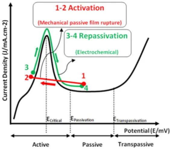
Film Rupture dissolution Model (FRM) describes intergranular SCC of stainless steel as a cyclic process of local surface activation by mechanical slipping and chemical dissolution of the freshly exposed surface at that location until it passivate again. The process is represented in Fig.1 and 2 [1,2,3].
SCC of stainless steel was analysed for its crystallography. Results reported {100} planes [4] for cleavage fracture. Others concluded that for sulfuric acid with chloride ions, {111} family of planes represents the fracture planes. Others reported {210} [5] and {211} and {310} [6,7].
In the current work, SCC will be in-lab produced so that its features of interest can be analyzed. The main analysis will concern the cracking crystallographical aspects using EBSD. This will reveal interesting information about cracking orientation relative to the surrounding/ruptured grains. Furthermore, the cracking fractography will be investigated by SEM imaging. This might lead to indications about cracking regime. For the applied and residual stress analysis, XRD technique was used to produce the corresponding applied/residual stress profile over the sample’s depth. The first analysis was dedicated to study the residual stress profile in the initial sheet of metal resulting from the manufacturing processes. After the application of stress, stress analysis was performed to check the evolution of stress profile due to this applied stress. Eventually, another residual/applied stress analysis was conducted to check the cracking effect on the residual and applied stress after SCC test has been performed.
Figure 1:Representation of FRM showing a crack propagation cycle of mechanical slip (1-2), chemical dissolution (2-3), and passivation (3-4).
Figure 2: Stainless steel polarization curve representing an activation/passivation cycle of SCC of stainless steel.
2 Experimental 2.1 Material used
304L Stainless Steel (SS) grade was selected to be used in these experiments. This is a widely used grade in commercial applications, and it has an equal importance in nuclear industry.
Spectromax was used to analyse the elemental composition of the alloy in hand as shown in table (1). Leco CS-300 combustion analyzer was used to measure the sulfur and carbon dose in the alloy. The analysis is summarized in table 1.
Table 1: The measured elementary composition of 304L stain less steel.
Element Fe Cr Ni Si Cu Mo Co N V Mn % by wt. 71,564 17,390 7,972 0,341 0,314 0,242 0,153 0,081 0,078 0,040 Element P C Sn Nb S As Ti Se Ca ∑ 𝑚
% by wt. 0,033 0,025 0,019 0,017 0,006 0,005 0,004 0,003 0,001 97.9
A tensile test in the rolling direction was conducted for this material. From this, the modulus of elasticity is given as E=210 GPa, while σ0.2 = 250 MPa is the elastic limit
corresponding to 0.2% ε, and eventually, the fracture limit is σR = 1000 MPa.
Due to the smooth elastic-plastic transition that this material shows, Ramberg-Osgood equation can be used to describe the mechanical behavior of this material [8]. Accordingly, the strain is given as:
𝜀 =𝜎𝐸+ 𝑘(𝜎𝐸)𝑛 Equation (1) The term 𝜎/𝐸 represents the elastic part of the strain, while 𝑘(𝜎/𝐸)𝑛 represents the plastic part. The constants n and K are material properties describing the strain hardening. Taking only the elastic part of the equation and taking the logarithm of both sides gives:
ln(𝜀𝑝) = ln(𝑘) + 𝑛ln(𝜎
𝐸) Equation (2)
This relationship represents a linear relationship between the plastic deformation and
𝜎/𝐸 in logarithmic basis. The slope of this line is equal to the constant n, and k is the exponential of its y-intercept. In the domain of interest of our current experiments, where ε < 5%, n and k are 8.23, and 5.4 X 10²⁰
2.2 Stress application
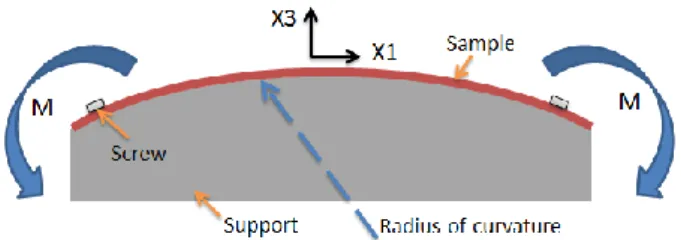
To apply certain value of tensile stress, the samples were elasto-plastically deformed using curved supports having different radii of curvature, as shown in Fig.3.
Figure 3: Side view of the support-sample assembly. Bending moment is applied to the sample resulting in a constant uniaxial stress.
By this assembly, the sample is subjected to constant bending moment by the two screws fixing it to the curved support. This creates an applied uniaxial stress on the central part of the sample. Assuming that the volume doesn’t change, the sections of the sample remain flat after deformation, and the stress is uniaxial, the stress tensor is reduced to 𝜎1; where 𝜎2 and 𝜎3 are negligible, and 𝜎12and 𝜎23are zero.
The deformation of the sample on the upper fibers; 𝜀𝑡𝑜𝑡, can be calculated using the relation:
𝜀𝑡𝑜𝑡 = 2𝑅𝑒 Equation (3)
In this equation, “e” is the sample thickness, and “R” is the radius of the curvature of the support. For deformations with a radius of curvature (800, 500, 333) mm, the strains calculated by eq.3 are (0.1, 0.16, 0.24) %ε respectively. By Hook’s law, this strain can be related to the stress as:
σ1 = Ee2R Equation (4)
This relation is valid only if the stress remains below the elastic limit.
For the 0.1% ε, using eq.4, the corresponding applied stress is equal to 210 MPa. However, the supports exerting higher deformations; 0.16 and 0.24 % ε, eq.4 gives 517 and 345 MPa respectively. This would count to the stress if the material was perfectly elastic. Due to plasticisation, the stress value would be lower than those calculated above. Equation 1 can be used to solve for the actual value of stress corresponding to the given applied deformation. This is possible by defining a parameter 𝛼 = 𝑘(𝜎𝑜𝐸)𝑛−4, which relates k and the yield strength of the material; 𝜎𝑜. Rewriting the second term of eq.1 using α, this gives:
𝑘(𝜎𝐸)𝑛 = 𝛼𝜎 𝐸(
𝜎 𝜎𝑜)
𝑛−1 Equation (5)
By making this replacement in eq.1, Ramberg-Osgood equation becomes:
𝜀 =𝜎𝐸+ 𝛼𝜎𝐸(𝜎𝜎
𝑜)
𝑛−1 Equation (6)
Having the values of the applied deformations 0.24 and 0.16%, the corresponding stresses can be calculated for by iterations using eq.6, which gives 280, and 250 MPa respectively.
2.3 AESEC method and electrochemical cell
In addition to classical immersion SCC tests, conventional electrochemistry was used to perform SCC tests. The electrochemical cell used was adapted from AESEC technique [9]. The assembly of this experimental technique allows a solution to be circulated/flow inside the electrochemical cell. Hence, the leaching solution is instantaneously taken away, holding the produced corrosion products with it, and a
new fresh solution is pumped to replace it. This can be connected to an ICP-OES spectrometer to get quantified information about the elementary dissolution rates, if required, which can aid to understand corrosion related phenomena.
2.4 Scanning Electron Microscope + EBSD
JSM-7100F scanning electron microscope was used to perform the electronic imaging. Oxford instruments EBSD detector is used to produce the crystallographic orientation maps. For imaging, the parameters used were: 15 kV acceleration voltage, and 20 mm working distance. Same settings were used for EBSD analysis, with a sample inclination equals to 70°.
2.5 X-Ray diffraction
Siemens D500 X-ray Power Diffraction (XRD) system was used to perform the residual-applied stress analysis using sin2ψ method [10]. Mn tube and Cr filter were used to fit with stainless steel experimental conditions. The tube was operated at 600 W (20 mA/30mV). Analysis were based on the diffraction of {311} planes of austenite, using 13 equally spaced ψ angles between -42.6° and 45°. To calculate the stress from the measured strain, the used X-ray elastic constants were 1/2S2hkl=6.98 MPa-1
and S1hkl= -1.87 MPa-1.
2.4 Experimental Procedure
The experimental work falls into two main categories. Immersion tests and AESEC cell tests. The following sections explain the experimental conditions used for them.
2.4.1 Immersion tests
The first is a classical immersion test where severe conditions were used of both solution concentration and applied stress. For this, part, two samples with R = (500, 333) mm were left in immersion for 21 days in 2 M H2SO4 and 2 M NaCl. The
purpose of these experiments is to get a severe attack, where the basic post analysis might be made. Based on these results, the conditions were modified to be more controlled for the next experimental set.
2.4.2 AESEC chemical cell tests
In the second experimental set, less chloride concentration, and less applied stress was used. Namely; 2 M H2SO4 and 0.5 M NaCl was used. For this case, the chemical
cell of AESEC system was used. These experimental conditions allowed more control in terms of experimental time, and exposed surface area. Using this, stressed and unstressed samples were subjected to OCP corrosion tests. The purpose is to in-lab produce SCC within a reasonable period of time; in an order of a day. In-situ analysis of the surface OCP potential evolution and leaching solution concentration is possible. Post analysis included SEM observation, EBSD, and XRD stress analysis. Experiments were performed at room temperature in 2 M H2SO4 solution with
different chloride concentrations (2 M and 0.5 M). The choice of the composition of the solution was based on the necessity to have a chloride content, which accelerates SCC production. However, the selection of sulphuric acid is due to its anion ability to give a great stabilizing effect on the repassivation process [11].
3 Results
3.1 Classical Immersion tests
Both samples showed visible cracks after the 21-day immersion SCC test. The following analysis was made to characterize the resulting samples.
3.1.1 Post-test observation by SEM
The topography of the upper surface and the cracks profiles has been observed by SEM. Fig.4-5 show the resulting images.
Figure 4: Upper surface, ε = 0.16% . Figure 5: Cross section, ε = 0.16% .
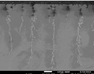
Since the produced cracks were very well developed in the depth of the sample, characterising the crack fractography of the produced cracks was of interest. For this, the sample of R500 was chosen. One of the cracks was open such that SEM analysis can be made for its facet. Fig.6 below shows the crack facet as marked by the green circle, below the dashed line. The surface with the pink circle is the sample’s upper surface.
Figure 6: The crack facet of , ε = 0.16%, 21-day immersion SCC test.
3.1.2 The EBSD map of crystallographic orientation around the cracks
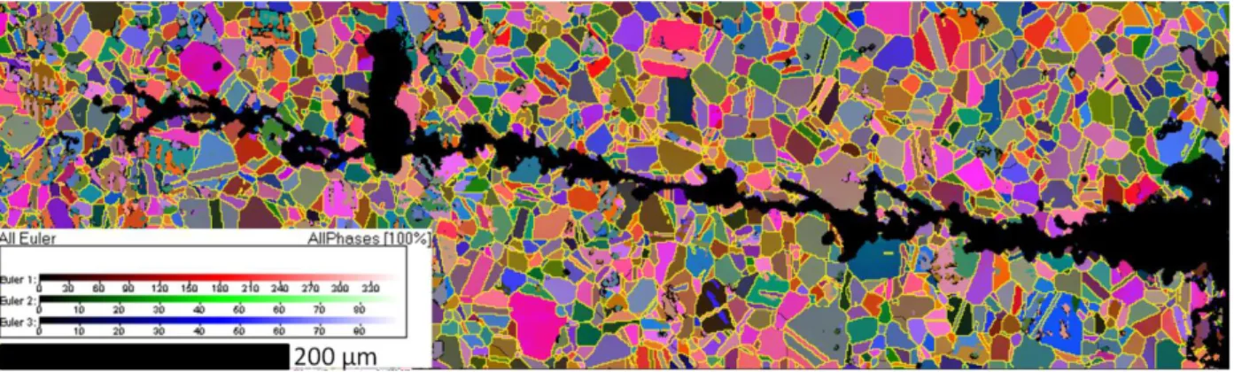
Three cracks were selected to be analysed in this section. The orientation map shown in Fig.7 is one of them. This is related to σ = 245 MPa applied stress sample.
Figure 7: EBSD map of crystallographic orientation around a SCC, σ = 245 MPa sample.
3.2 OCP SCC tests using AESEC chemical cell.
For this experimental set, SCC tests of different periods have been performed. All these tests were performed using the same conditions, while only the test duration was changed for each of them. In the first part, experiments were made to study the SCC kinetics. Another test was made to study the effects related to residual/applied stress before and after SCC.
3.2.1 SCC kinetics
For the different tests performed here, the upper surface and cross section were observed using SEM imaging. Fig.8 shows the evolution of corrosion with time on the upper surface, and on the crack initiation and growth.
Figure 8: SCC evolution with time on the upper surface, σ = 210 MPa.
3.2.2 The stress profile obtained by XRD.
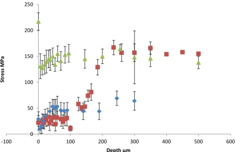
The XRD analysis over the sample depth profile gave the curves indicated in Fig.9. The crude metal sheet shows to have residual stresses due to manufacturing processes. The effect of the applied stress is very pronounced on the curve representing the sample after deformation.
Figure 9: XRD residual – applied profile stress analysis over the sample’s depth.
4 Discussion
4.1 Immersion SCC test of R300 and R500 samples. 4.1.1 Corrosion regimes and dissolution traces
Fig. 6 shows different corrosion regimes. Regime “A “ corresponds to an aggressive corrosion after the crack propagation over the entire experiment. Following this is regime “B” where the three parallel lines indicated by the arrows in Fig.6 are traces of the step wise mode of crack propagation. This might correspond to locations of slip system activation, followed by dissolution of freshly exposed surface. This stands as evidence in favor of the FRM, as described in Fig. 1 and 2. Such results were found by [12]. The last regime is “C”, which represents the rapid propagation of SCC, where the cracks have grown to make large decohesive crack coalesce with cleavage and fluting features. Such results were found by [13,14]. Fig.6 helps identify these regimes on the cross-section. This cracking behavior is in agreement with cracking kinetics described by [15].
4.1.2 Effect of stress on crack initiation sites
The sample having higher stress value had more crack initiation sites. This result reinforces the role of stress on crack initiation. Higher stress value will have a higher probability to activate slipping systems on the surface, and hence, crack nucleation locations. However, conclusion concerning the effect of stress on crack length cannot be made here due to the very long experimental time in such aggressive environment. Same thing can be said about the features of the upper surface topography after the test, which was totally altered by general corrosion after cracking as seen in Fig. 3.
4.1.3 The rupture planes orientations
Having the EBSD map for the crystallographic orientation of the grains made it possible to analyse the cracking planes. The interest was to check if the cracking plane has any crystallographic features. Thus, the ruptured grains were isolated. From the crack path, a line is chosen representing the top view of the cracking plane. An assumption is made here is that this plane is perpendicular to the sample cross-sectional plane. To verify if this assumption is valid, step-wise polishing was
0 50 100 150 200 250 -100 0 100 200 300 400 500 600 Str e ss M Pa Depth µm σ1, after 44 h SCC test σ1, 0.1% strain σ1, before deformation
performed. Five EBSD maps were produced with 5 µm polishing step between each of them. The results revealed that the perpendicularity assumption is applicable to most of the grains, and only a slight correction was required for certain cases. This correction was limited when needed to no more than 10°, and it proved to give more representative results. The EBSD map shown here is one map among three that were used in this analysis. The required information to determine the orientation of the cracking plane can be stated as: the three Euler angles defining the crystallographic orientation of the cracked grain, and the crack orientation based on a straight line drawn in the path of the crack. From these three maps, 20 grains were analysed. Four plane families has been identified as cracking plane, namely: {110}, {111},{211}, {100}. The rupture plane showed to be preferential on {110} and {111} plane families, with percentages of 48% and 37% respectively. According to FRM, SCC takes place as repetition of cycles of passive film breakdown, dissolution, until it repassivates again. Slipping system in face centered cubic crystals is activated over {111} planes. This result confirms previous studies performed by [3,16,17]. On the other hand, {110} family of planes will be the cracking plane in FCC system if equal number of dislocations pile-up on the primary and conjugate {111} slip planes [15, 18].
4.2 OCP SCC tests using AESEC chemical cell 4.2.1 XRD and stress relaxation due to cracking.
From the obtained stress profiles, we see that the metallic sheet used in these experiments has an initial residual tensile stress. This stress is propably due to manufacturing processing, such as rolling. The average of the measured stress on the surface was 33 MPa. The sample was deformed using the support of 800 mm radius. For the deformed sample, the same measurements were made on the upper surface giving a stress value equals to 213 MPa. This value of stress represents the elastic limit of the material in hand, and it confirms the theoretical calculation made by eq.4 corresponding to this amount of deformation.
The interest was to measure the stress value after the SCC test. The average crack length for this period of SCC test is about 95 µm, and the maximum possible crack length is about 175 µm. This is directly reflected on the measured stress profile over the sample’s depth. From the upper surface (depth = 0) to the point at 100 µm, the stress falls to a close value to the initial residual stress in the bulk of the material. And starting from this point, the measured stress starts to increase gradually with depth. This gradual increase stops at depth equals to 175 µm, after which the stress profile shows a platform until 500 µm depth representing the applied stress value. This is clarified in table 3.
Table 3: The residual/applied stress vlues as measured by XRD.
Depth 0.0 5 to 100 µm 100 to 175 µm 175 to 500 µm Initial, 0.0% ε 29 MPa 40 MPa 45 MPa 65 MPa
1% ε 213 MPa 143 MPa 150 MPa 150 MPa
1% ε, after 44 h SCC
29 MPa 25 MPa Gradual increase from 25-160 MPa
160 MPa
4.2.2 SCC kinetics
Four samples with σ = 210 MPa were subjected to SCC OCP tests using 2 M H2SO4
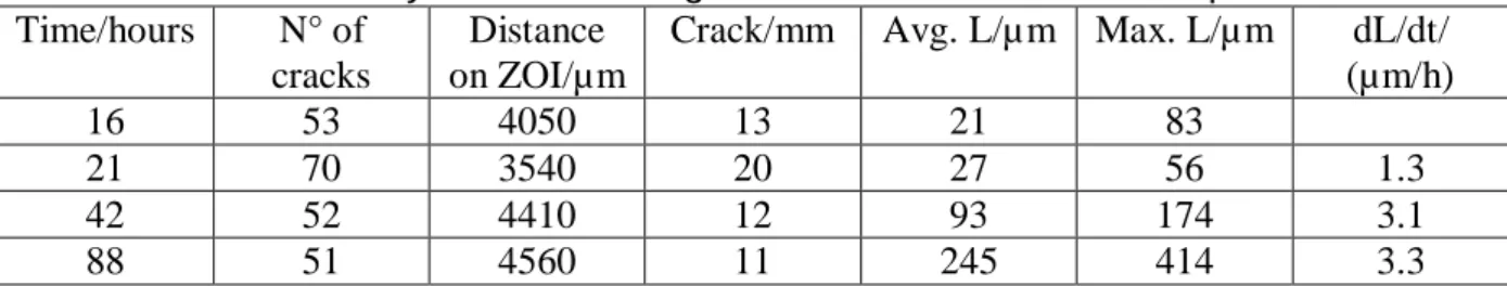
were studied in order to measure the length of the cracks found in each of them. The table below makes a summary about the obtained results.
Table 4: statistical analysis of crack length for the different SCC tests performed. Time/hours N° of
cracks
Distance on ZOI/µm
Crack/mm Avg. L/µm Max. L/µm dL/dt/ (µm/h)
16 53 4050 13 21 83
21 70 3540 20 27 56 1.3
42 52 4410 12 93 174 3.1
88 51 4560 11 245 414 3.3
In this table, we have the average length of the cracks observed at the cross sections of each sample. The fact that the crack has a semi-elliptical shape makes the interpretation of the measured lengths not straight forward. The location at which the cross section has been made might have passed through the mid of this semi-elliptical shape, or at the edge where it’s almost seen as a pit, or somewhere in between which makes it appear as a shorter crack than some others surrounding it. Thus, to compare between SCC tests of different periods, the criterion of average crack length might be taken with caution. Another effective way of comparison is the maximum crack length.
The crack propagation rate is calculated based on the average crack length evolution between a test and the next interval. This revealed that the crack propagation rate is not linear. For the interval between 16 h to 21 h, it was 1.3 µm/ hour. While for the next two intervals between 21 h to 42 h, and 42 h to 88 h, the propagation rate was about three times this value.
The number of cracks seems to be the same for all the experiments, except for the experiment of 21 h. This indicates that the number of crack initiation sites is not increasing with time. This result is reasonable; since crack initiation on the upper surface has a vital requirement, which is the existence of stress. We have seen from the XRD stress analysis after the SCC that due to cracking, the surface gets back to the stress value corresponding to the residual stress in the bulk material. Hence, cracks initiation happens more or less simultaneously, and then they propagate simultaneously with different propagation rates due to the different local stress values at different crack tips. Some of those propagating cracks might heal due to passivation, or to stress relaxation caused by neighboring cracks.
5 Conclusions
SCC has been in lab produced using a sulphuric acid solution containing chloride ion. The resulting cracks were analysed using SEM, EBSD, and XRD techniques. The analysis revealed a clear crystallographic nature of cracking. The main conclusions that can be drawn are as follows:
Crystallographic orientation analysis revealed two types of preferential rupture planes; {110}, {111} with percentages around 48%, 37% respectively. For face centered cubic crystals, {111} planes are those over which slipping occurs. However, rupture planes could be of {110} family due to equal dislocation-pile-up on the primary and conjugate {111} planes. This result comes in favor of FRM concerning dissolutions taking place on the planes corresponding to slipping systems.
SEM observation shows that crack propagation has a non-linear relation with exposure time, where it stars with low propagation kinetics within the period
between 16-21 h, and goes to three times this speed between the period 21-88 h.
XRD analysis revealed that the initial metal sheet has tensile residual stress around 30 MPA attributed to the manufacturing processes.
The effect of cracking the surface after SCC tests causes stress relaxation to the basic residual stress value existing in the bulk material. This was the case between the surfaces, until 95 µm depth which represents the average crack length obtained.
A gradual stress increase was observed between the depth of 95 µm to the depth of 175 µm, which represents the maximum crack length obtained at this period. After this depth, the material gets back to 160 MPa, which corresponds to the applied stress value.
Acknowledgment: Special thanks to Dr. Fabrice Guittonneau for his constructive ideas and support throughout the the SEM and EBSD experiments and analysis.
6 References
[1] E.W. Hart, Surfaces and Interfaces II, Syracuse University Press, (1968), p 210.
[2] H.J. Engle, in The Theory of Stress Corrosion Cracking in Alloys, North Atlantic Treaty Organization, (1971).
[3] J.C. Scully, Corrosion Science, 15 (1975), p 207.
[4] R. E. Reed and H. W. Staehle, Corrosion, 23 (1967), p 117. [5] M. Marek and R. F. Hochman, Corrosion, 27 (1971), p 361.
[6] R. J. Asaro, A. J. West and W. A. Tiller, Stress Corrosion Cracking and Hydrogen Embrittlement of Iron Base Alloys. NACE, Houston, TX (1977), p 1115.
[7] R. Liu, N. Narita, C. Altstetter, H. Birnbaum and E. N. Pugh, Metakk. Trans. A11A, (1980),p 1563.
[8] Ramberg, W. and Osgood, W.R., Description of stress-strain curves by three parameters. Technical Note No 902, National Advisory committee For Aeronautics, Washington DC, (1943).
[9] K. Ogle, J. Baeyens, J. Swiatowaska, P. Volovitch, Electrochimicha Acta, 54 (2009), p 5163.
[10] L. Castex, J.L. Lebrun, G. Maeder, and J.M Sprauel. Détermination des contraintes résiduelles par diffraction des rayons x. Technical report, ENSAM de Paris, (1981). [12] R.N. Parkins, C.M. Rangel, and J. Yu, Metall, Trans. A, Vol 16A, (1985), p 1671.
[11] F.J. Graham, H.C. Brookes, J.W. Bayles, J. Appl. Electrochem. Nucleation and growth of anodic films on stainless steel alloys II. Kinetics of repassivation of freshly generated metal surfaces. 20 (1990): p 45.
[13] A.J. Rusell and D. Tromans, Metall. Trans. A, Vol 10A, 1979, p 1229.
[14] D.A. Meyn and E.J. Brooks, in Fractography and Material Science, STP 733, L.N. Gilbertson and R.D.
Zipp, Ed., American Society for Testing and Materials, 1981, p 5. [15] R.N. Parkins, Corrosion 46, (1990), p 178.
[16] J. D. Harston and J. C. Scully, Corrosion NACE, vol. 26, NO. 9 (1970).
[17] W. D. Robertson and A. S. Tetelman, Strengthening Mechanics in Solids. American Society for Metals, Metals Park, OH (1962), p 2017.