MATH 564 Project Report. Analysis of Desktop Virtualization Capacity with. Linear Regression Model

MATH 564 Project Report

Analysis of Desktop Virtualization Capacity with

Linear Regression Model

Hongwei Jin CWID:A20288745

1.

Problem Describe

a) Background Information

At the beginning, let me declare the terminology of “virtualization”. In computing, virtualization is the creation of a virtual (rather than actual) version of something, such as a hardware platform, operating system (OS), storage device, or network resources. What’s more, the so-called “desktop virtualization” is separating a personal computer desktop environment from a physical machine using the client–server model of computing. It means you can use your “computer” just as normal type wherever and whenever you are with kinds of devices, such as laptop, TV, tablets, and even mobiles. All your data will be saved on server safely.

With the development of cloud computing, more and more companies using virtualization technology to improve the efficiency of work and cut off devices budgets. In the business field, almost all the companies want to build their own virtualization system efficiently and economically.

So a direct question from the manager is that if deploying a server, how many users can it provide at the same time?

b) Data Description1

The most important data I care about is the average delay time (ms) of all users which denoted as

y

, the number of users at the same time, which denoted

x

₁ and the cores of server provided for those users, which denoted as

x

₂.

Here I get some kind of data from our human testing under control of the server, which means I ask some people to operate their own virtual desktop at the same time with a sequence of operations. However, it takes a long time to finish a round test. So I develop software to simulate the daily operation of humans. It will speed up to get the goal.

c) Objective

In my prior work, I have analysis the performance of server. However, there still exist some omits. How can I prove that the software is trustable? If not, all the analysis will be fault.

The report of this report will provide evidences statistically by using the linear regression model that the software is trustable when measuring the capacity of server.

2.

Analysis

1 _{The project is a subproject of a real project conducted by ICT (China Academy of Sciences) and Huawei. All the}

a) Method[1]

The problem of this project can be viewed as reliability engineering, which is one of the fields of engineering statistics. Compared with linear regression model and time series models, the report will choose linear regression model to convince the goal. b) Numerical Output and Figures

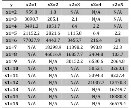
We can first look at the original data of testing from Table 1. Here are some

comments: first, some data are not available due to either the delay time is too large, or the delay time is so small. For example, when 1 core of server supports the service with more than 7 users, it will delay more than 77027 ms, and when 3 cores of server support less than 3 users is a waste of resource. It doesn’t make any sense; then a general idea from the data is that for each fixed number of cores, the delay time will increase exponentially or quadratically; at last, with the increase of cores, the average delay time of users will decrease exponentially or quadratically; what’s more, range of data is quite large.

The data of

x

₂



1

,

2

,

3

,

4

is come from the human test result. It reflects the pattern of benchmark of human normal operation on the server. While the data of

x

₂



5

is the simulated one from software I developed.

Table 1 Original data from testing result

y x2=1 x2=2 x2=3 x2=4 x2=5

x1=2 959.8 1.8 N/A N/A N/A

x1=3 3898.7 285.1 2.1 N/A N/A x1=4 3491.3 1051.7 64 2.2 N/A x1=5 21152.2 2821.6 1115.8 6.4 2.2 x1=6 77027.9 4443.7 3455.7 216.4 24 x1=7 N/A 18298.9 11398.2 993.8 22.3 x1=8 N/A 46016.9 16857.7 2404.8 103.7 x1=9 N/A N/A 30152.2 6530.6 2064.8

x1=10 N/A N/A N/A 5052.1 3260.1

x1=11 N/A N/A N/A 5394.3 8227.4

x1=12 N/A N/A N/A 21007.7 13470.3

x1=13 N/A N/A N/A N/A 16749.7

x1=14 N/A N/A N/A N/A 18380.3

x1=15 N/A N/A N/A N/A 36579.4

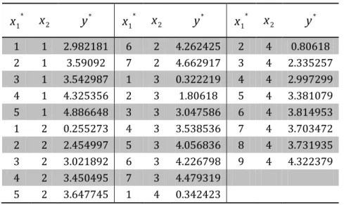
According to the comment above, we can do Box-Cox transformation of the

original data y , what more we should take the relation between core number and delay time. So we have our first model.

y

y

*

_

log

_and

₁

2 1 * 1



x



x



x

become like Table 2.

Table 2 Data after Box-Cox transformation * 1

x

x

2

y

*

x

1*

x

2

y

*

x

1*

x

2

y

* 1 1 2.982181 6 2 4.262425 2 4 0.80618 2 1 3.59092 7 2 4.662917 3 4 2.335257 3 1 3.542987 1 3 0.322219 4 4 2.997299 4 1 4.325356 2 3 1.80618 5 4 3.381079 5 1 4.886648 3 3 3.047586 6 4 3.814953 1 2 0.255273 4 3 3.538536 7 4 3.703472 2 2 2.454997 5 3 4.056836 8 4 3.731935 3 2 3.021892 6 3 4.226798 9 4 4.322379 4 2 3.450495 7 3 4.479319 5 2 3.647745 1 4 0.342423

Then start fit the model with simplest one with least square estimation:

ε

x

β

x

β

β

y







2 2



* 1 1 0 * Here are some results from JMP.

Figure 1 Actual by Predicted Plot

From the Figure 1, we can obtain that the

y

*predicted probability is smaller than 0.0001.

Table 3 Summary of Fit

RSquare 0.819074

RSquare Adj 0.8046

Root Mean Square Error 0.588202 Mean of Response 3.142725 Observations (or Sum Wgts) 28

From the Table 3, we can obtain that the RSquare is larger than 81.9%, which means almost 81.9% can be explained by this model.

Table 4 Analysis of Variance

Source DF Sum of Squares Mean Square F Ratio Prob > F Model 2 39.157450 19.5787 56.5890 <.0001* Error 25 8.649528 0.3460

C. Total 27 47.806979

From the ANOVA table above, we can obtain that the model has large F-ration and small Probability.

Table 5 Parameter Estimates

Term Estimate Std Error t Ratio Prob>|t| Intercept 2.5889443 0.324383 7.98 <.0001* x1* 0.5337144 0.052114 10.24 <.0001* X2 -0.610592 0.105979 -5.76 <.0001*

From the parameter estimate table, we can obtain that all the parameters are all significant.

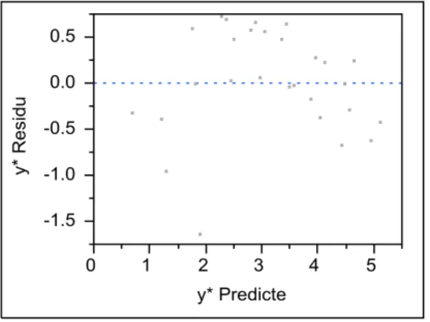
Figure 2 Residual by Predicted Plot

From the residual plot, we can obtain that there are some outlier plots, which are row 6 and row 13. Obviously, we should remove the outlier rows to fit the model again.

Figure 3 Residual by Predicted Plot after removing outliers

the estimated parameter are significant with probability <0.0001. The residual plot indicates that the residual are randomly distributed.

Can we improve the model with interactions? So we consider a model with parameter interactions.

ε

x

x

β

x

β

x

β

β

y









2



* 1 3 2 2 * 1 1 0 *

However, if we fit the model with interactive parameters, we will find that the interactive parameters have small F-ratio, large probability, which means there is no need to build an interactive model.

Table 6 Parameter Estimates with interactives

Term Estimate Std Error t Ratio Prob>|t| Intercept 2.977551 0.249223 11.95 <.0001*

x1* 0.4480481 0.043935 10.20 <.0001*

x2 -0.583795 0.08064 -7.24 <.0001*

(x1*-4.38462)*(x2-2.73077) 0.0200322 0.036711 0.55 0.5908

There is still no need to add self-interactive parameters. The probability of such parameter is large, so it is not an significant parameter in the model.

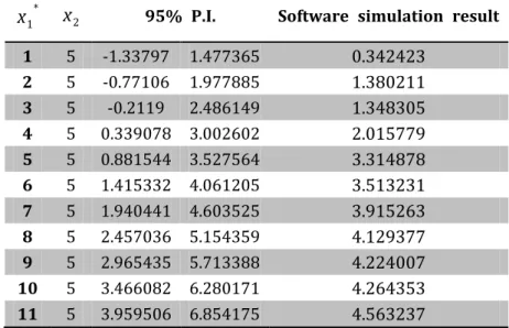
Then we analysis how trustable the software simulation is?

First, we get the 95% point prediction intervals of

x

₁*



1

,...,

11

and

x

2



5

, which can compare with the result of software estimation.

Table 7 Model PI v.s. Software simulation result *

1

x

x

2 95% P.I. Software simulation result

1 5 -1.33797 1.477365 0.342423 2 5 -0.77106 1.977885 1.380211 3 5 -0.2119 2.486149 1.348305 4 5 0.339078 3.002602 2.015779 5 5 0.881544 3.527564 3.314878 6 5 1.415332 4.061205 3.513231 7 5 1.940441 4.603525 3.915263 8 5 2.457036 5.154359 4.129377 9 5 2.965435 5.713388 4.224007 10 5 3.466082 6.280171 4.264353 11 5 3.959506 6.854175 4.563237

From the Table 7, we can obtain that every data of come from the software are in the range of 95% prediction interval of the model. Which means the software is almost trustable, and it can be used in the later works.

c) Summary of the Result

ε

e

ε

e

y

_

β0β1(x1x21)β2x2

_

_

(β0β1)β1x1(β2β1)x2

_

Where,

y

means the delay time (ms),

x

_{1 means the number of users at the same}

time and

x

₂means cores of server provided for those users.

Then through some analysis the residual and compare interactive models, we have the final model above. Even though it is a simple model, but it may be the best model to fit the data. At last, I analysis the results of software simulation and the 95% P.I. to draw the conclusion that the software, which developed to simulations the work of human being, is trustable.

I used the software to test a single server (16 cores) can contain almost 27 users at the same time, if we assume that one user can bear the delay time of 8000ms.

3.

Conclusion

a) Pros and Cons

i. Pros

 This is a simple model using linear regression model. We should build up models as simple as possible.

 It statistically proves that such software can be used in the system.

 For engineering statistics, it is an innovative one to analysis some kind of software is trustable in a particular work.

ii. Cons

 There is not such mass data from the test both in human being or software.

 It should compare the data both in C.I. and P.I.

 It may use another engineering statistic method, though I don’t know. b) Improvement and Notation

i. Method Choose

There are other kind of method related to engineering work[3]_{, such as DOE,} quality control, time and methods engineering, reliability engineering,

probabilistic design, and system identification. It is obvious that the design of testing is dynamic, so a much more reliable method can be choose to measure it. ii. Testing data

Even though there is a set of data, it is not large enough such that I can measure more patterns and characteristics from the data. Since it is conducted in other institution, I cannot do it again to improve it.

Reference

[1]. Bowerman, O’Connell, Koehler. Forecasting, Time Series, and Regression (fourth edition). Thomson Brooks/Cole, 2005.

[2]. Tao Jiang, Rui Hou, Lixin Zhang etc, Micro-architectural Characterization of Desktop Cloud Workloads. IISWC: San Diego, 2012