Robust modelling of count data

(1)

Technische Universität Dortmund

Fakultät Statistik

Robust Modelling of Count Data:

Applications in Medicine

Doctoral Thesis

Submitted by

Hanan Abdel kariem Abdel latif Elsaied

From Egypt

Supervisor:

Prof. Dr. Roland Fried

(2)

(3)

iii

To my family

and

to all members, who took part in the January 25 Revolution in Egypt

(4)

ACKNOWLEDGEMENT

First of all I would like to express my deepest gratitude to my supervisor, Professor Dr. Roland Fried for his continuous encouragement, patience, guidance and amiability throughout this work, without which this thesis would not have been accomplished. In Addition to my supervisor, I am deeply grateful to PD Dr. Sonja Kuhnt, who accepted to be the second referee. Also to Professor Dr. Katja Ickstadt, who accepted to be the heading of my commission.

I would especially like to thank Dr. Christian H. Weiss who gave me the references, which I asked. I am also grateful to Professor Dr. Konstantinos Fokianos, who gave me some comments on my dissertation before the discussion.

I would especially like to thank every one at the statistics department at the univer-sity in Dortmund, in particular, Dipl.-Stat. Tobias Liboschik who gave me the functions, which he implemented in R to remove outliers in Chapter 5. And my colleagues at work Arsene Ntiwa, Oliver Morell, Anita Thieler, Katrin Hainke and Dr. Daniel Vogel for their help. My thanks go to Sebastian Krey, who helped me in R, and Sabine Bell, who helped me from the first day I came to Germany. Also I am grateful to Omniah Abdulazim and Nadja Bauer, who I knew lately in our department for their help.

Further, I thank all of my friends who encouraged me all during the years I was working on my thesis. I would especially like to thank Doaa Elaidi, Haiam Elkatry from Egypt and Marina Umar Muchtar, Rohmatul Fajriyah from Andonisa. Also my best friends far away Seham Nabil, Hanaa Shehata, Mona Nazieh, and Professor Dr. Safaa Abdeldayem. And of course, I am also deeply grateful to all members of my family, my parents Abdel kariem Elsaied, Samia Abou zyed and my brothers Khaled, Sameh who are far away, for their encouragement and support.

Last but not least, I would definitely like to thank my husband Mohamed Elenany and my sons Ziad and Moaz, who stay with me through the difficult moments during this work and for their encouragement and support.

(5)

v

Abstract

M-estimators as modified versions of maximum likelihood estimators and their asymp-totic properties play an important role in the development of modern robust statistics since the 1960s. In our thesis, we construct new M-estimators based on Tukey’s bisquare function to fit count data robustly. The Poisson distribution provides a standard frame-work for the analysis of this type of data.

In case of independent identically distributed Poisson data, M-estimators based on the Huber and Tukey’s bisquare function are compared to already existing estimators imple-mented in R via simulations in case of clean data and of additive outliers. It turns out that it is difficult to combine high robustness against outliers and high efficiency under ideal conditions if the Poisson parameter is small, because such Poisson distributions are highly skewed. We suggest an alternative estimator based on adaptively trimmed means as a possible solution to this problem. Our simulation results indicate that a modified version of the R-function glmrob with external weights gives the best robustness prop-erties among all estimation procedures based on the Huber function. A new modified Tukey M-estimator provides improvements over the other procedures which depend on the Tukey function and also those which depend on the Huber function, particularly in case of moderately large and very large outliers. The estimator based on adaptive trim-ming provides even better results at small Poisson means.

Furthermore, our work constitutes a first treatment of robust M-estimation of INGARCH models for count time series. These models assume the observation at each point in time to follow a Poisson distribution conditionally on the past, with the conditional mean being a linear function of previous observations and past conditional means. We focus on the INGARCH(1,0) model as the simplest interesting variant. Our approach based on Tukey’s bisquare function with bias correction and initialization from a robust AR(1) fit provides good efficiencies in case of clean data. In the presence of outliers, the bias-corrected Tukey M-estimators perform better than the unbias-corrected ones and the condi-tional maximum likelihood estimator. The construction of adequate Tukey M-estimators or the development of other robust estimators for INGARCH models of higher orders remains an open problem, albeit some preliminary investigations for the INGARCH(1,1) model are presented here.

Some applications to real data from the medical field and artificial data examples indicate that the INGARCH(1,0) model is a promising candidate for such data, and that the issue of robust estimation tackled here is important.

Keywords: Count data; Poisson model; INGARCH models; GLM models; Huber M-estimator; Tukey M-M-estimator; Robustness; Asymptotic properties; Medical applica-tions.

(6)

(7)

List of Figures

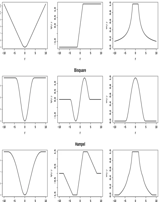
1.1 Thesis outline . . . 3 2.1 ρ , ψ and ω functions (from left to right) for Huber, Tukey and Hampel

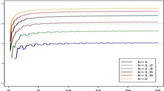
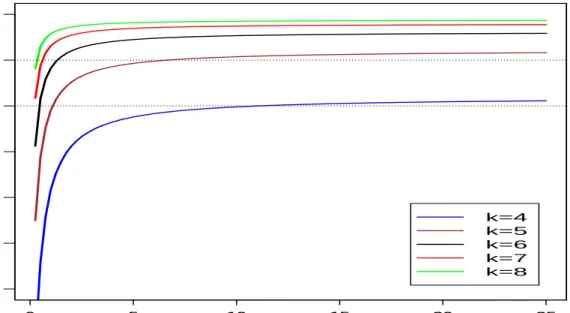
proposals . . . 11 3.1 Relative asymptotic efficiency of the Huber M-estimator relatively to the

sample mean as a function of underlying true mean θ for several tuning constantsk. . . 23 3.2 Relative asymptotic efficiency of the Tukey M-estimator relatively to the

sample mean as a function of underlying true mean θ for several tuning constantsk. . . 25 3.3 Comparison of the sample biases of all Huber procedures with several

tun-ing constants k in case of an increasing percentage of additive outliers of size 5 and a Poisson distribution with mean 2, sample size n=100. . . 29 3.4 Comparison of the relative efficiencies measured by the mean square error

of all Huber procedures with several tuning constants k relatively to the sample mean as a function of the underlying true mean, sample size n=100. 30 3.5 Comparison of the relative efficiencies measured by the mean square error

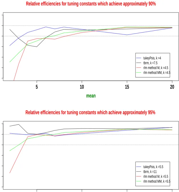
of all Huber procedures relatively to the sample mean as a function of the underlying true mean for refined values of the tuning constants k, sample size n=100. . . 32 3.6 Comparison of the relatively efficiencies for the Huber M-estimators at

tun-ing constants, which achieve approximately 90% or 95% level of efficiency (from top to bottom). . . 33 3.7 Comparison of the biases of the Huber procedures tuned to achieve 90%

level of efficiency in case of a Poisson with mean 2 and the sizes of the additive outliers being 5, 10 and 30 (from top to bottom). . . 36 3.8 Comparison of the biases of the Huber procedures tuned to achieve 90%

level of efficiency in case of a Poisson with mean 5 and the sizes of the additive outliers being 5, 10 and 30 (from top to bottom). . . 37 3.9 Comparison of the biases of the Huber procedures tuned to achieve 95%

level of efficiency in case of a Poisson with mean 2 and the sizes of the additive outliers being 5, 10 and 30 (from top to bottom). . . 38

(12)

3.10 Comparison of the biases of the Huber procedures tuned to achieve achieve 95% level of efficiency in case of a Poisson with mean 5 and the sizes of the additive outliers being 5,10 and 30 (from top to bottom). . . 39 3.11 Comparison of the sample biases of all Tukey procedures in the case of

additive outliers of size 5 and a Poisson distribution with mean 2. . . 41 3.12 Comparison of the relative efficiencies of the Tukey procedures relatively

to the sample mean as a function of the underlying true mean for several tuning constants k. . . 42 3.13 Comparison of the relative efficiencies of the Tukey procedures relatively

to the sample mean as a function of the underlying true mean for refined values of the tuning constants k. . . 44 3.14 Comparison of the relative efficiencies of the Tukey procedures at tuning

constants which achieve approximately 90% or 95% level of efficiency (from top to bottom). . . 45 3.15 Comparison of the biases of the Tukey based procedures tuned to achieve

90% level of efficiency in case of a Poisson with mean 2 and the sizes of the additive outliers being 5, 10 and 30 (from top to bottom). . . 47 3.16 Comparison of the biases of the Tukey based procedures tuned to achieve

90% level of efficiency in case of a Poisson with mean 5 and the sizes of the additive outliers being 5, 10 and 30 (from top to bottom). . . 48 3.17 Comparison of the biases of glmrob with external weights and tukeypois,

both tuned to achieve 90% level of efficiency in case of a Poisson with mean 2 and the sizes of the additive outliers being 5, 10 and 30 (from top to bottom). . . 51 3.18 Comparison of the biases of tukeypois, huberpois, glmrob and glmrob with

external weights, tuned to achieve 95% efficiency in case of an additive outlier of increasing size (left) and in case of the additive outliers of size 3 for tukeypois, size 5 for glmrob with external weights and of size 8 for the others (right), in case of a Poisson with mean 2, sample size n=100. . . . 52 3.19 Relative efficiencies for tukeypois, glmrob, trimmeanfit and roptest

mea-sured by the percentage mean square error relatively to the sample mean with several tuning constants k, n=100 . . . 55 3.20 Comparison of the biases of tukeypois, glmrob, trimmeanfit and roptest

with several tuning constants k, in case of a Poisson with mean 0.5 and the sizes of the additive outliers being 2 and 5, respectively. . . 56 3.21 Comparison of the biases of tukeypois, glmrob, trimmeanfit and roptest

with several tuning constants k, in case of a Poisson with mean 2 and the sizes of the additive outliers being 5 and 10, respectively. . . 57 4.1 Simulated biases of tukeypois, glmrob with external weight, trimmeanfit

and roptest tuned to achieve 95% level of efficiency in case of one transient outlier of increasing size from 1 to 20 in a Poisson time series with mean 2. 67

(13)

LIST OF FIGURES xiii

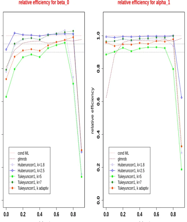
4.2 Simulated biases of tukeypois, glmrob with external weight, trimmeanfit and roptest tuned to achieve 95% level of efficiency in case of two transient outliers of increasing size from 1 to 20 in a Poisson time series with mean 2. 68 4.3 Simulated relative efficiencies of glmrob, Huber and Tukey M-estimators

with different tuning constants k relative to the conditional maximum likelihood estimator for β0 (left) and α1 (right) as a function of the true

α1, n=100. . . 77

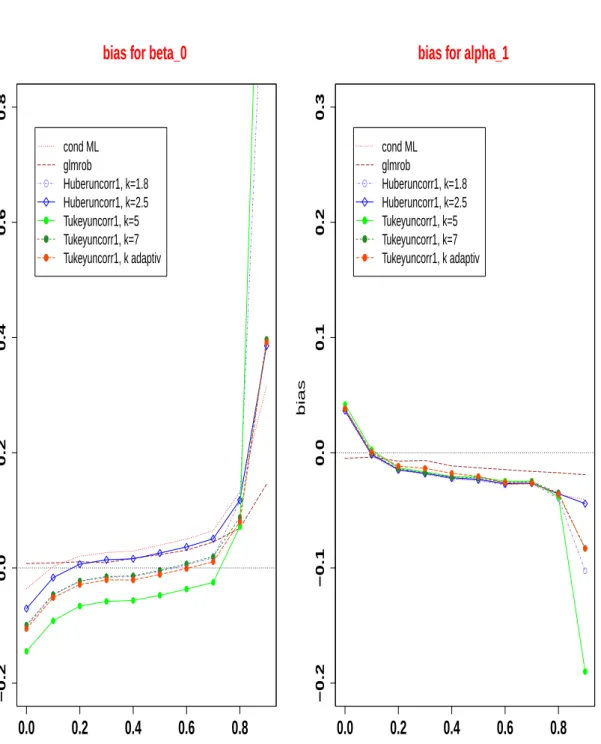
4.4 Simulated biases of the conditional maximum likelihood estimator, glmrob and of Huber and Tukey M-estimators with different tuning constants k for β0 (left) and α1 (right) as a function of the trueα1, n=100. . . 78

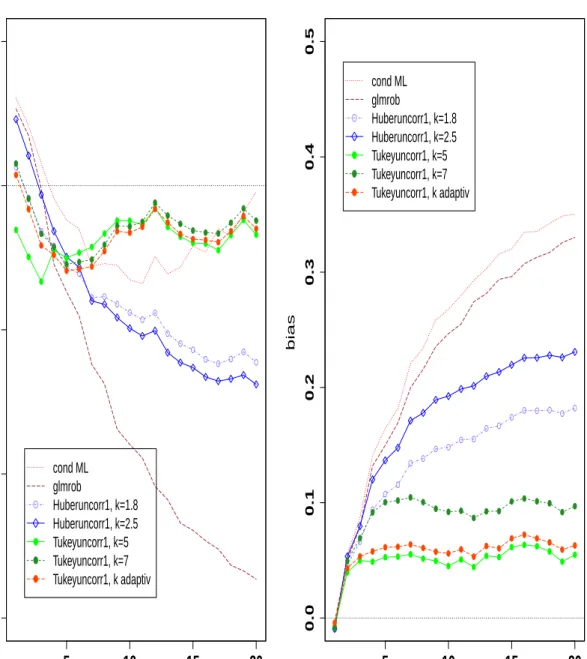
4.5 Simulated biases of the conditional maximum likelihood estimator, glmrob and of Huber and Tukey M-estimators with different tuning constants k forβ0 (left) andα1 (right) in case of one transient outlier of increasing size

with β0 = 1 andα1 = 0.4, sample size n=100. . . 79

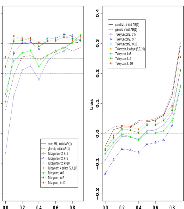
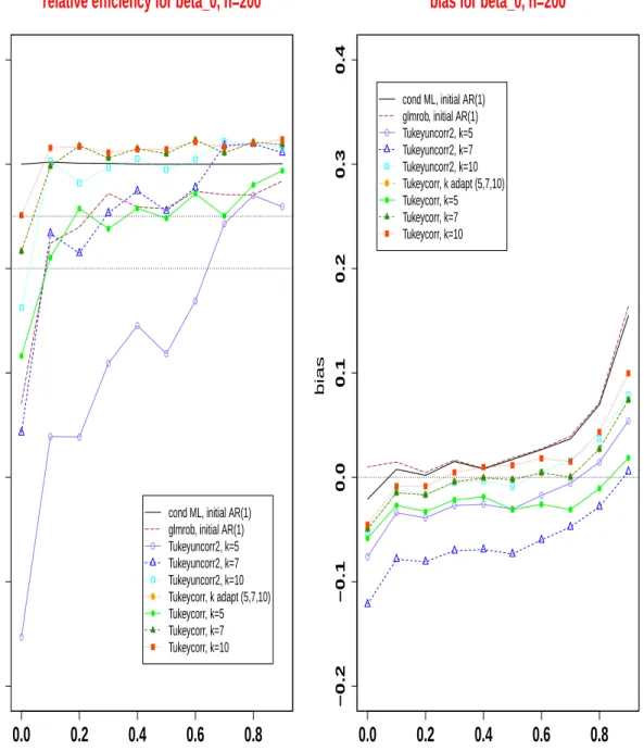
4.6 Simulated biases forβ0 (right) and relative efficiencies for β0 (left) of

glm-rob, corrected and uncorrected Tukey M-estimators with different tuning constants k, relatively to the conditional maximum likelihood estimator, as a function of the true value ofα1, forβ0 = 1, n=100. . . 82

4.7 Simulated biases forβ0 (right) and relative efficiencies for β0 (left) of

4.8 Simulated biases for α1 (right) and relative efficiencies for α1 (left) of

glmob, corrected and uncorrected Tukey M-estimators with different tun-ing constants k, relatively to the conditional maximum likelihood estima-tor, as a function of the true value of α1, forβ0 = 1, n=100. . . 84

4.9 Simulated biases forα1 (right) and relative efficiencies forα1 (left) of

4.10 Boxplots of the conditional maximum likelihood estimator and uncorrected Tukey M-estimators with tuning constant k = 5 for β0 (top) and α1

(bot-tom) estimated from INARCH(1) with true values β0 = 1 and α1 = 0.4,

5000 data sets of sizes 100, 200, and 500 (from left to right). . . 86 4.11 QQ-plots of the conditional maximum likelihood estimator and

uncor-rected Tukey M-estimators with tuning constant k = 5 for β0 estimated

from INARCH(1) with true valuesβ0 = 1 and α1 = 0.4, 5000 data sets of

sizes 100, 200, and 500 (from left to right). . . 87 4.12 QQ-plots of the conditional maximum likelihood estimator and

uncor-rected Tukey M-estimators with tuning constant k = 5 for α1 estimated

from INARCH(1) with true valuesβ0 = 1 and α1 = 0.4, 5000 data sets of

(14)

4.13 Simulated biases of the conditional maximum likelihood estimator, glm-rob, corrected and uncorrected Tukey M-estimators with different tuning constants k for β0 (left) and α1 (right) in case of one transient outlier of

increasing size with true valuesβ0 = 1 and α1 = 0.4, sample size n=200. . 91

4.14 Simulated biases of the conditional maximum likelihood estimator, glm-rob, corrected and uncorrected Tukey M-estimators with different tuning constants k for β0 (left) and α1 (right) in case of an additive outlier of

4.15 Simulated biases of the conditional maximum likelihood estimator, glm-rob, corrected and uncorrected Tukey M-estimators with different tuning constants k for β0 (left) and α1 (right) in case of increasing numbers of

additive outliers of increasing sizes with true values β0 = 1 and α1 = 0.4,

sample size n=200. . . 93 4.16 Simulated biases of the conditional maximum likelihood estimator,

glm-rob, corrected and uncorrected Tukey M-estimators with different tuning constants k for β0 (left) and α1 (right) in case of increasing numbers of

additive outlier of fixed size [4σ] with true values β0 = 1 and α1 = 0.4,

sample size n=200. . . 94 4.17 Boxplots of the conditional maximum likelihood estimator and Tukey

M-estimators with tuning constant k = 7 for β0, α1 and β1 (from left to

right) estimated from INGARCH(1,1) with true values β0 = 1, α1 = 0.3

and β1 = 0.4, 500 data sets of size 200. . . 101

5.1 Monthly number of poliomyelitis cases in the United States for the period 1970 to 1983. . . 108 5.2 Polio data (solid black line) and data after outliers removal (dashed green

line). Step 1: AO at time 35 (vertical red line), step 2: TS at time 7 (vertical blue line), step 3: TS at time 113 (vertical brown line), step 4: LS at time 167 (vertical yellowgreen line). . . 110 5.3 Artificial Polio data (solid black line) and data after removal of outliers

(dashed green line). Step 1: AO at time 35 (vertical red line), step 2: TS at time 7 (vertical blue line), step 3: TS at time 113 (vertical brown line). 112 5.4 Monthly number of cases of campylobacterosis infections from January

1990 to the end of October 2000 in the north of the Province of Quebec, Canada. . . 113 5.5 Campy data (solid black line) and data after removal of outliers (dashed

green line). Step 1: LS at time 84 (vertical red line), step 2: TS at time 100 (vertical blue line). . . 115 5.6 Artificial campy data (solid black line) and data after outliers removal

(dashed green line). Step 1: TS at time 100 (vertical red line), step 2: LS at time 84 (vertical blue line). . . 117 A.1 Equation (A.5) . . . 125

(15)

LIST OF FIGURES xv

B.1 Simulated biases (bottom) and relative efficiencies (top) of corrected and uncorrected Huber M estimator with different tuning constantskrelatively to the conditional maximum likelihood estimator forβ0 (left) andα1(right)

as a function of the true α1, for β0 = 1 and n=200. . . 134

B.2 Simulated biases of the conditional maximum likelihood estimator and of corrected and uncorrected Huber M-estimators with different tuning constants k for β0 (left) and α1(right) in case of an additive outlier of

B.3 Simulated biases of the conditional maximum likelihood estimator and of corrected and uncorrected Huber M-estimators with different tuning constants k for β0 (left) and α1(right) in case of a transient outlier of

B.4 Simulated biases of the conditional maximum likelihood estimator and of corrected and uncorrected Huber M-estimators with different tuning constants k for β0 (left) and α1(right) in case of increasing numbers of

additive outliers of increasing sizes with true values β0 = 1 and α1 = 0.4,

sample size n=200. . . 137 B.5 Simulated biases of the conditional maximum likelihood estimator and

of corrected and uncorrected Huber M-estimators with different tuning constants k for β0 (left) and α1(right) in case of increasing numbers of

additive outlier of fixed size with true values β0 = 1 andα1 = 0.4, sample

(16)

(17)

List of Tables

2.1 ρ, ψ and ω functions for Huber, Tukey and Hampel proposals . . 10

4.1 Results of the Tukey M-estimators and the conditional maximum likeli-hood estimator in case of clean data withβ0 = 1, α1 = 0.3 and β1 = 0.4. 100

4.2 Results of the Tukey M-estimators and the conditional maximum likeli-hood estimator in case of 3 additive outliers with β0 = 1, α1 = 0.3 and

β1 = 0.4. . . 103

β1 = 0.4. . . 104

β1 = 0.4. . . 105

5.1 Parameter estimates for the polio data (left) and for the cleaned polio data (right) . . . 109 5.2 Parameter estimates for the artificial polio data (left) and for the cleaned

artificial polio data (right) . . . 111 5.3 Parameter estimates for the campy data (left) and for the cleaned campy

data (right) . . . 114 5.4 Parameter estimates for the artificial campy data (left) and for the cleaned

artificial campy data (right) . . . 116

(18)

List of abbreviations Abbreviation Meaning P age ABP Asymptotic breakdo wn p oin t 12 A O A dditiv e outlier 110 ARE Asymptotic relativ e efficiency 23 BP Breakdo wn p oin t 12 condlik est Conditional maxim um lik eliho o d function for INAR CH(1) mo del 72 condlik est11 Conditional maxim um lik eliho o d function for INGAR CH(1,1) mo del 72 FBP Finite breakdo wn p oin t 12 GES Gross-error sensitivit y 14 glmrob with externa l w eigh ts glmrob in the R-pac kage robustbase using external w eigh t function 28 h ub erp ois Hub er estima tor for i.i.d. P oisson data 24 Hub ercorr Hub er estima tor with bias correction for INAR CH(1) mo del 134 Hub eruncorr Hub er estima tor without bias correction for INAR CH(1) mo del 75 tuk eyp ois T uk ey es timator for i.i.d. P oisson data 26 IF Influence function 13 INGAR CH In teger-v alued genera lized autoregressiv e conditional heteroscedasticit y mo del 59 LS Lev el shift outlier 110 p oissmall Initial estimator for i.i.d. P oisson data 24 RMSE Ro ot me an square error 29 trimmeanfit A daptiv e trimming estimator 54 robP oisTSh ub er1 Hub er func tion without bias correction and with indep endence initialization for INAR CH(1) 72 robP oisTSh ub er2 Hub er func tion without bias correction and with initialization from the AR(1) for INAR CH(1) 72 robP oisTSh ub er3 Hub er func tion with bias correction and with initialization from the AR(1) for INAR CH(1) 72 robP oisTStuk ey1 T uk ey fun ction without bias correction and with indep endence initialization for INAR CH(1) 72 robP oisTStuk ey2 T uk ey fun ction without bias correction and with initialization fr om the AR(1) for INAR CH(1) 72 robP oisTStuk ey3 T uk ey fun ction with bias correction and with initialization from the AR(1) fo r INAR CH(1) 72 robP oisTStuk ey11 T uk ey es timator without bias correction for INGAR CH(1,1) mo del 99 robP oisTStuk ey22 T uk ey es timator without bias correction for INGAR CH(1,1) using indep enden t initialization 99 robP oisTStuk ey33 T uk ey es timator with bias correction for INGAR CH(1,1) using ARM A( 1,1) initialization 100 SC Sensitivit y curv e 13 TS T ransien t shif t outlier 110 T uk eyuncorr T uk ey es timator without bias correction for INAR CH(1) mo del 80 T uk eycorr T uk ey es timator with bias correction for INAR CH(1) mo del 80

(19)

Chapter 1 Introduction

Robust statistics provides inference methods, which are not sensitive to unusual observa-tions or other small deviaobserva-tions from ideal models. Finding the best fit to the majority of the data is one of the most important aims of robust methods.

M-estimators are a general class of robust estimators and their asymptotic properties played an important role in the development of modern robust statistics since the 1960s, where the most important property is that for any asymptotically normal estimator exists an asymptotically equivalent M-estimator, see Staudte and Sheather (1990, Page 116). In general there are two main approaches to finding robust M-estimators described in Peracchi (1990). The first one is Huber’s minimax approach, see Huber (1964, 1981). The second one is Hampel’s infinitesimal approach, see Hampel (1968) and Hampel et al. (1986). Both approaches assume a parametric model for the observations and try to con-struct estimators that perform well over a neighborhood of the assumed model. Huber’s approach is to consider a neighborhood of the assumed parametric model and then to safeguard within that neighborhood in a minimax sense. This approach also described in Kordzakhia et al. (2001) is based on the minimization of some functional of the likelihood process, namely so-called Huber’s ρ functions, see Section 2.1 and Section 2.2. Hampel’s approach focuses on the asymptotic behavior of an estimator in an infinitesimal neigh-borhood of a given model. In our work, we follow the first approach to finding robust estimators, but we use modified versions of likelihood functions, which are suitable for our model and we use estimators computed using the second approach for the purpose of comparison, as we will see later in Chapter 3.

This thesis considers the problem of robust modelling for count data, where the Poisson model provides a standard framework for the analysis of this type of data. It consists of six chapters and the relationship between them is illustrated in Figure 1.1. The first chapter is this introduction and the outline of the other chapters is as follows:

• In Chapter 2, we review some concepts for location M-estimators in robust estima-tion theory such as their definiestima-tion, types, properties and computaestima-tion.

• In Chapter 3, we construct new Tukey M-estimators with bias correction of the Poisson mean in case of i.i.d. data. We propose a new algorithm for estimating the

(20)

mean of the Poisson distribution, which is based on the Tukey function. We mod-ify the R-function glmrob by adding a bias correction term and external weights. Then we compare modified bias-corrected M-estimators based on the Huber and the Tukey functions to already existing estimators implemented in R via simulation in case of clean and additive outliers data. We will finish this chapter by considering alternative estimators as a solution to the problem of combining high robustness against outliers and high efficiency relatively to the sample mean when the true mean is small.

• In Chapter 4, we introduce robust M-estimation for so called INGARCH models for count time series data in the presence of outliers, where we focus on robust esti-mation for the INGARCH(1,0), or more briefly INARCH(1), model. We start with the definition and the properties of these models. We apply conditional maximum likelihood as a classical approach to estimate the parameters of these models. We discuss robust estimation of the marginal mean in case of time series data from INGARCH models using our best functions given in Chapter 3 for i.i.d. Poisson data. Then we modify the classical estimation approach by giving robust estima-tors for the parameters of the INARCH(1) model. We investigate some of the basic properties of these estimators. Afterwards we compute the estimates using some functions, which we have implemented in R, and compare them via simulations in case of clean and contaminated Poisson time series data. We will finish this chapter by trying to extend robust estimation to more general INGARCH models.

• In Chapter 5, we apply our methods proposed in Chapter 4 to two real data exam-ples in the medical field. The first example is the poliomyelitis data. The second example is the campylobacterosis data. We start with an analysis of the poliomyeli-tis data. We give a description of these data, then we fit an INGARCH(1,0) model to them using conditional maximum likelihood as a non robust method and Tukey M-estimation as a robust method for parameter estimation. After that, we fit an INGARCH(1,0) model using the same methods but after having cleaned the data from outliers. To verify the reliability of our proposed methods, we analyse an artificial data example generated to resemble the poliomyelitis data. We fit an INGARCH(1,0) model to the artificial data using the same methods as for the poliomyelitis data, then we fit an INGARCH(1,0) model again but after having cleaned the artificial data from outliers. For the campylobacterosis data, we repeat what we did for the poliomyelitis data.

• In Chapter 6, we provide a summary, conclusions and an outlook.

Each chapter starts with a short description of its contents. Additionally, we begin Chapter 3 and Chapter 4 with a brief review of the previous treatments in the literature for the topics treated in these chapters.

We use R software version 2.11.1 (2010-05-31). Under R, we use packages "MASS", "robustbase", "dplR" and "ROptEst". Along with this dissertation comes a CD, which contains the .pdf of this document and the codes in R, which we wrote to calculate our estimates, to run our simulations and to plot our figures.

(21)

3

M-estimation

Introduction & Concepts

Chap

. 3

Chap. 5

(

Application

)

Chap. 4

Chap

. 1

Chap

. 2

Ind. Data

Dep. Data

(22)

(23)

Chapter 2 Basic concepts of location

M-estimators

The purpose of this chapter is to present some basic concepts of location M-estimators in robust estimation theory, which we will need afterwards. We start by giving a definition of location M-estimators. Then we present Huber’s M-estimators and Tukey’s biweight or bisquare M-estimators as different types of M-estimators. Afterwards we review criteria used for studying whether robust estimators have good properties: qualitative robust-ness, quantitative robustrobust-ness, and infinitesimal robustness. We finish this chapter by the computation of location M-estimators with previously computed dispersion.

2.1 Definition of location M-Estimators

M-estimators naturally estimate M-measures of location, so we can define them through the following three parts:

• Location model

• Measures of location

• M-Estimators

We first consider the simplelocation modelas described in Maronna et al. (2006, Page 17),

Xi =µ+ui (i= 1, ..., n), (2.1)

where the outcome Xi of each observation depends on the true value of µ and on some

random error ui, with u1, ..., un being assumed to be independent and identically

dis-tributed random variables with the same symmetric distributionF0, which is symmetric

to 0. It follows that X1, ..., Xn are independent with common distribution function F,

where

(24)

F(x) =F0(x−µ), x∈ R (2.2)

A measure µ maps a class _z of distribution functions F onto the real line (R) by con-structing µ(F). According to Staudte and Sheather (1990, Page 101), a measure µ is called a measure of location if for any constants a and b and random variable X with distribution F holds:

• µ(X+b) = µ(X) +b (location equivariance).

• µ(−X) = −µ(X) (symmetry).

• X ≥0 implies µ(X)≥0.

• µ(aX) = aµ(X) for alla >0.

Bickel and Lehmann (1975) require measures of location to be stochastic order preserving, so they added

• IfX is stochastically larger than Y, thenµ(X)≥µ(Y).

We can use the classical estimator of µ, e.g., least squares or maximum likelihood meth-ods, assuming the data to come from the same normal distribution,F0 ∼N(0, σ2), which

implies that F ∼N(µ, σ2) if there are no outliers.

Applying the maximum likelihood method, the likelihood function for a realizationx1, ..., xn

of X1, ..., Xn is L(x1, ..., xn;µ) = n Y i=1 f0(xi−µ), (2.3)

withf0 being a density of F0. The maximum likelihood estimate (MLE) ofµis the value

ˆ

µ- depending on (x1, ..., xn) - that maximizesL(x1, ..., xn;µ),

ˆ

µ= ˆµ(x1, ..., xn) =argmaxµL(x1, ..., xn;µ), (2.4)

where ”argmax” stands for "the value maximizing the function".

IfF was exactly a normal distribution, the MLE which is the sample mean would be an optimal estimator. But if F is only approximately normal, then our goal is an estimator that is almost as good as the mean when F is exactly normal. To achieve this goal, we use modified versions of maximum likelihood methods for estimation, such that ˆµis close toµ with high probability, e.g., M-estimators.

M-estimators are a broad class of estimators which are obtained as the solution of the

problem of minimizing certain objective functions of the data or as the root of a system of equations equating certain functions of the data to 0. Given observationsx1, ..., xn, an

(25)

2.1 Definition of location M-Estimators 7

X

ρ(xi, µ) (2.5)

where theρfunction measures the agreement between an observationxi and any possible

value ofµ. Usingρ(x, µ) =−logf0(x, µ), i.e. the negative logarithm of the model density,

gives the maximum likelihood estimator.

If we assume that ρ has a derivative ψ with respect to its second argument, ψ(xi, µ) = ∂

∂µρ(xi, µ), then an M-estimator can be defined as the solution of the following equation

for ˆµ

n

X

i=1

ψ(xi,µˆ) = 0. (2.6)

According to Maronna et al. (2006, Page 23), we can calculate ˆµ using the maximum likelihood estimation as a special case of M-estimation for model (2.1) assuming the scale parameter σ to be known, e.g., σ = 1, as follows:

Since the logarithm is an increasing function if f0 is everywhere positive, (2.4) can be

written as ˆ µ= ˆµ(x1, ..., xn) = argminµ n X i=1 ρ(xi−µ), (2.7)

If ρis differentiable, differentiating (2.7) with respect to µyields

n

X

i=1

ψ(xi−µˆ) = 0 (2.8)

Note that if f0 is symmetric, then ρ is even and hence ψ is odd.

Generally, we have the following possible solutions of (2.8) according to the type of ψ:

• ifψ is monotone nondecreasing withψ(−∞)<0< ψ(∞), a solution to (2.8) exists and all solutions form an interval since ρ is convex.

• Ifψ is continuous and strictly increasing, the solution is unique.

• If ψ is discontinuous, a solution to (2.8) might not exist and in this case we shall interpret (2.8) to mean that the left-hand side changes its sign at ˆµ.

• Ifψ is not a strictly monotone function, then there can be more than one solution of (2.8).

Using different structures ofρ and ψ functions gives different types of estimates of µ, for example the mean and the median:

If F0 =N(0,1), then f0(x) = √1₂_πe−

x2

2 , and apart from a constant we have for the MLE

ρ(x) = x₂2 and ψ(x) = x, and equation (2.8) becomes

n

X

i=1

(26)

which has ˆµ= ¯x, the sample mean, as its unique solution.

If F0 is the double exponential distribution, f0(x) = ₂1e−|x|, then for the MLEρ(x, µ) = |x−µ|, ψ(x, µ) =sign(x−µ), and any sample median of x1, ..., xn will be a solution of

(2.8), what is equivalent to

n

X

i=1

sign(xi−µˆ) = 0 (2.10)

Under normality the sample mean is the most efficient estimator forµ, while the median has asymptotic efficiency _π2 ≈ 64%, since the asymptotic variance of the sample median is π/2, see Maronna et al. (2006, Page 26). On the other hand, the median is a robust measure of central tendency while the mean is not.

Now our problem is, how can we choose appropriate ρ or ψ functions, which give us the best compromise between efficiency and robustness? One of the most popularψ functions is the Huber function

ψ(ri) =    ri, |ri| ≤k k·sign(ri), |ri|> k (2.11) where for i = 1, ..., n, ri = xi −µ is the residual of xi and k is a tuning constant to be

determined suitably.

The calculation of the Huber location estimate defined in (2.11) is commonly done by iteratively reweighted least squares (IRWLS), derived from writing the solution of equa-tion (2.8) as a weighted mean with weights depending on the distances between the data points and the current solution as follows:

Define the weight function W(ri)

W(ri) =ψ(ri)/ri =    1, |ri| ≤k k/|ri|, |ri|> k (2.12) Rewrite (2.8) as n X i=1 W(ri)(xi−µˆ) = 0 (2.13) so that ˆ µ= Pn i=1ωixi Pn i=1ωi (2.14) with ωi =W(ri). If W(ri) is bounded and nonincreasing forri >0, IRWLS converges to

a solution of (2.8).

For Huber’s ψ function, choosing a larger value of k increases the efficiency but reduces the robustness to outliers. Now our problem becomes how can we choose a reasonable value of k? If the model distribution F is a normal distribution with a unit scale, it is reasonable to choose the tuning constant k of the Huber function within the interval [1,3], since such distributions rarely generate values with distances from the mean larger than 3 (standard deviations), whereas all values within the range [−1,1] are typical. We will give later on more details about ψ functions and the results of applying these functions for different choices of the tuning constants.

(27)

2.2 Types of M-Estimators 9

IfF depends on an unknown scale parameterσ, we can derive M-Estimators in two ways: 1. with previous estimation of dispersion,

2. simultaneous M-Estimates of location and dispersion.

In these cases, k can be chosen as a corresponding multiple of an estimate ˆσ, which can be calculated a-priori or simultaneously, see Maronna et al. (2006, Page 36). We will discuss these options with some details in Section 2.4.

2.2 Types of M-Estimators

Several types of M-estimators have been developed depending on the choice of ρ or ψ functions. One usually tries to obtain ρ or ψ functions, which lead to some desirable properties. If ρ is differentiable, the computation of the estimate ˆµ is usually easier. If the derivative ψ of ρ is continuous and strictly monotone increasing, there is a unique solution like in case of Huber’s ψ function. When ψ is not monotone a solution of (2.8) is called a redescending M-estimator. According to Staudte and Sheather (1990, Page 118), redescending M-estimators are popular since they have some additional de-sirable properties. Their ψ functions are non decreasing near the origin but decrease for large arguments. Many of them satisfy ψ(x) = 0 for all xwith|x| ≥k, wherek is a finite number which is called the minimum rejection point.

Another property is that they can be quite efficient and have a high breakdown point if we find the solution by iteration, beginning with an initial estimator with a high break-down point, and unlike other outlier rejection techniques they do not suffer from masking effects. Their efficiency is due to the fact that they completely reject large outliers, but use the exact values of all reasonable observations, as opposed to the median. This is because their ψ function is chosen to redescend smoothly to 0.

Examples for this type of estimators:

• Hampel’s three part M-estimators

• Tukey’s biweight or bisquare M-estimators

Table 2.1 and Figure 2.1 show the differentρ,ψ andω(weights) functions, for the Huber, Hampel and Tukey proposals, which are the most popular ones.

From Table 2.1, we find that Hampel’s ψ function is more complicated than the Huber and Tukey functions since it needs fixing three tuning constantsa,b andcinstead of only one constant. So in our study, we will concentrate on the Huber function and the Tukey function, which have been successfully used in a wide variety of applications. Under the normal model with a unit scale, Tukey’sψfunction needs larger values ofkbetween 3 and 5, because k does not limit the range of typical, but the range of plausible observations generated from the normal model.

(28)

T able 2.1: ρ , ψ and ω functions for Hub er, T uk ey and H amp el prop osals Criterion ρ ( r i₎ ψ ( r i₎ = ∂ ∂ µ ρ ( r i₎ ω ( r i₎ = ψ ( r i₎ /r i range Hub er 1 2 r 2 i r i 1 | r i_| ≤ k k | r i_| − 1 2 k 2 k · sig n ( r i₎ k / | r i_| | r i_| > k T uk ey’s biw eigh t 1 − [1 − ( r i k ) ₂ ] ₃ r i_[1 − ( r i k ) ₂ ] ₂ [1 − ( r i k ) ₂ ] ₂ | r i_| ≤ k 1 0 0 | r i_| > k Hamp el r 2 i r i 1 | r i_| ≤ a 2 a | r i_| − a 2 a · sig n ( r i₎ a | r i_| a < | r i_| ≤ b a (2 c | r i_| − r 2 i₎ c − b − 7 6 a 2 a · sig n ( r i₎₍ c − | r i_| ) c − b a | r i_| · ( c | r i_| ) / ( c − b ) b < | r i_| ≤ c

(29)

2.2 Types of M-Estimators 11 −10 −5 0 5 10 0 2 4 6 8 10 12 r ρ ( r ) −10 −5 0 5 10 −1.0 0.0 0.5 1.0

Huber

r ψ ( r ) −10 −5 0 5 10 0.0 0.2 0.4 0.6 0.8 1.0 r w ( r ) −10 −5 0 5 10 0 1 2 3 r ρ ( r ) −10 −5 0 5 10 −1.0 0.0 0.5 1.0

Bisquare

r ψ ( r ) −10 −5 0 5 10 0.0 0.2 0.4 0.6 0.8 1.0 r w ( r ) −10 −5 0 5 10 0 2 4 6 r ρ ( r ) −10 −5 0 5 10 −1.5 −0.5 0.5 1.5

Hampel

r ψ ( r ) −10 −5 0 5 10 0.0 0.2 0.4 0.6 0.8 1.0 r w ( r )

Figure 2.1: ρ , ψ and ω functions (from left to right) for Huber, Tukey and Hampel proposals

(30)

2.3 Properties of M-Estimators

There are three basic concepts used to establish whether robust estimators have good properties:

• Qualitative robustness

• Quantitative robustness

• Infinitesimal robustness

Qualitative robustness:

The definition of qualitative robustness is very closely related to continuity of the statis-tic in the weak topology viewed as a functional. Hampel et al. (1986, Page 99) relate continuity and qualitative robustness with each other, where they note that qualitative robustness is closely related, but not identical with, a nonzero breakdown point. Hampel (1968) calls an estimator qualitatively robust if its sampling distribution is equicontinous. That is, roughly stated, a small change in distribution of the observations should cause only a small change in the distribution of the estimator.

Quantitative robustness (global reliability):

The general idea here is to measure quantitatively how the effect of a small change in the underlying distributionF changes the distribution of an estimator or statistic ˆθ. The breakdown point (BP) addresses this property. The BP concepts have been presented by Maronna et al. (2006, Page 58) as follows: Let X = (x1, ..., xn) be a data set and

let ˆθn be an estimator of the parameter θ, which belongs to a given parameter space Θ.

The finite-sample breakdown point (FBP) is the largest fraction of contamination m/n, such that ˆθn is bounded away from the boundary of Θ, if at most m data points are

changed arbitrarily. More formally: Let d: Θ×Θ→ R+

0 be a distance measure and call N(X, m) ={Z= (z1, ..., zn) : #{i:zi 6=xi} =m}. Then the FBP of ˆθ at the sample X

is n(ˆθ,X) = 1 nmax{m :∃K, d(ˆθn(Z), ˆ θn(X))< K ∀Z∈ N(X, m)}. (2.15)

The asymptotic contamination breakdown point (ABP) of an estimate ˆθ at F, denoted by ∗(ˆθ, F), is the largest fraction ∈ (0,1) of contamination, such that ˆθ is bounded away from the boundary of Θ for all distributions in the corresponding contamination neighborhood. More formally: Letd: Θ×Θ→ R+0 be a distance measure andN(F, ) := {(1−)F +G, G ∈ G} be a contamination neighborhood of F, where G is a family of contamination distributions. Then

∗(ˆθ, F) = sup{ >0 :∃K ∈ R, d ˆ θ(F),θˆ((1−)F +G) < K ∀G∈ G} (2.16)

In most cases of interest, the FBP does not depend on X and tends to the ABP when

(31)

2.3 Properties of M-Estimators 13

Note that both the sample mean and the sample variance have an FBP and ABP of 0 if the parameter space is R. On the other hand, the median has a breakdown point of 50% asymptotically if the parameter space is R, because at least half of the observations need to be moved arbitrarily far away before the median becomes completely wrong. For location M-estimators with monotonic but not necessarily oddψ function, the break-down point is

∗(ˆθ;F) = min(k1, k2) k1 +k2

(2.17) where k1 =−ψ(−∞) andk2 =ψ(∞) are the limits of ψ as its argument goes to −∞or ∞. If ψ is odd as for the Huber M-estimator, then k1 = k2 and ∗ = 0.5. For all

prac-tical purposes the bisquare M-estimator with previous scale (median absolute deviation, MAD) has ∗ = 0.5, while for simultaneous estimation, ∗ is usually lower than 0.5, see Maronna et al. (2006, Page 60).

Infinitesimal robustness (local stability)

Infinitesimal robustness shows us what happens if we add one more observation with value x0 to a large sample. The Influence Function (IF) measures the effect of an infinitesimal

perturbation, where IF in its finite sample version is known as the Sensitivity Curve (SC). The SC is defined in Maronna et al. (2006, Page 55) as follows: Let x1, ..., xn be

an i.i.d. sample from a distribution F and ˆθn an estimator of a parameter θ, then

SC_θˆ n(x1, ..., xn, x0) = (n+ 1)[ˆθn+1(x1, ..., xn, x0)− ˆ θn(x1, ..., xn)] = ˆ θ (1− 1 n+1)Fn+ 1 n+1δx0 −θˆ(Fn) 1 n+1

TheSC is computed by calculating the estimator ˆθn as a function of the empirical

distri-bution (Fn = Σni=1δxi/n) with and without an observation, whereδx0 is the point-mass at

the pointx0, and is proportional to the size of the sample. This means theSC describes

the effect of an individual observation on the estimator for a specific data set. When we let the sample size n tend to infinity (asymptotic behavior), we usually have ˆθn

p

−

→θˆ∞(F),

where ˆθ∞(F) is the asymptotic value of the estimate at F, and the resulting limit is the IF. According to Hampel (1974), the IF of an estimator ˆθ at a distribution F is

IF_θˆ(x0, F) = lim→0 ˆ θ∞ (1−)F +δx0 −θˆ∞(F) , (2.18)

where ˆθ∞ is a functional on a set of reasonable distributions (a contamination

neighbor-hood of F).

Note that the SC is obtained if F is replaced by the empirical distribution Fn, which

assigns mass _n₊₁1 to each of (x0, x1, ..., xn), and setting to _n+11 .

For location M-estimators with bounded and continuousψ function, Croux (1998) shows that for eachx0

(32)

SC_θˆ_n(x0) a.s. −−→IF_θˆ(x0, F) The IF of an M-estimator is IF_θˆ(x0, F) =− ψ(x0,θˆ∞) B(θ, ψ) (2.19)

withB(θ, ψ) = _∂θ∂Eψ(X, θ). Equation (2.19) shows an important connection between the IF and the ψ function of an M-estimator. TheIF provides a lot of information on the estimators. According to Maronna et al. (2006, Page 62), the most important one being that the IF gives us a picture of the asymptotic bias caused by a small contamination of size in the data (robustness stability). To show this: Consider a contamination neighborhood of Fθ with parameter θ, and ˆθ an estimator of θ, such that

N(Fθ, ) := {(1−)Fθ+G, G∈ G},

whereG is a family of contamination distributions. Then the asymptotic bias of ˆθ at any F ∈ N(Fθ, ) is

B(F, θ) = ˆθ∞(F)−θ

and the maximum asymptotic bias (M B) is

M B_θˆ(, θ) = sup{|B(F, θ)|:F ∈ N(Fθ, )}

where the maximum bias is related to the IF via M B_θˆ(, θ)≈·γ(ˆθ, θ)

for small values of, where γ(ˆθ, θ) is the gross-error sensitivity (GES) of ˆθ at θ, which is equal to

γ(ˆθ, θ) = max

x0

|IF_θˆ(x0, Fθ)|. (2.20)

If the parameter space is the whole set of real numbers, the relationship between M B and BP is

∗(ˆθ, Fθ) = max{≥0 :M B_θˆ(, θ)<∞}

Note that two estimators may have the sameBP but different M Bs.

For M-estimators with nondecreasing and bounded ψ function, let Fµ(x) = F0(x−µ),

where F0 is symmetric about 0, k = ψ(∞) and < 0.5, then the maximum bias is the

(33)

2.3 Properties of M-Estimators 15

EF0ψ(x, b) =

k

1−, (2.21)

see Maronna et al. (2006, Page 79).

Secondly, Martin (1978) shows that the IF provides an intuitively appealing representa-tion for a robust estimator from which the asymptotic distriburepresenta-tion of the estimate may be formally deduced. Under some regularity conditions, ˆθn may be represented as

ˆ θn=θ+ 1 n n X i=1 IF_θˆ(xi, F) +Rn (2.22)

and often the remainder term satisfies n12R_n−→d 0. Then the difference

√

n{[ˆθn−θ]−_n1 Pni=1IF_θˆ(xi, F)}

converges to zero in probability, so that we have the approximation

√

n(ˆθn−θ) a

∼ N(0, V_θˆ(θ))

i.e. ˆθn−θ is asymptotically normal with parameters

EF[IF_θˆ(X, F)] = 0 (i.e. E(ˆθn)→θ)

and

V_θˆ(θ) =EF(IF_θˆ(X, F))2 (2.23)

This formula shows that a bounded IF implies a bounded asymptotic variance.

Maronna et al. (2006, Page 64) define the asymptotic relative efficiency (ARE) of ˆθ atθ as the ratio of variances as follows:

ARE(θ) =Vmin(θ)/V_θˆ(θ) (2.24)

where Vmin(θ) is the smallest possible asymptotic variance within a reasonable class of

estimators (e.g. equivariant ones) or Vmin(θ) = min{V_θˆ(θ) : ˆθ is a "reasonable" estimator

of θ}. Under reasonable regularity conditionsVmin(θ) is usually achieved by the MLE.

At the normal model, M-estimators with the Huber function (2.11) have an ARE larger than redescending M-estimators if we choose the constants to obtain the same maxi-mal bias. For several symmetric, wider tailed distributions, suitable redescending M-estimators are slightly more efficient than M-M-estimators with the Huber function, and for the Cauchy distribution redescending M-estimators are much more efficient (about 20% more) than the Huber estimator. This is because they completely reject large aberrant observations, while the Huber estimator effectively treats them like moderate outliers, see Staudte and Sheather (1990, Page 119).

(34)

If F does not belong to the family Fθ but is in a neighborhood of Fθ, F ∈ N(Fθ, ), the

bias will dominate the variance component of MSE for n large since (ˆθn−θ) a

∼ N(b, w/n)

with b = ˆθ∞(F)−θ being the asymptotic bias and w the asymptotical variance of ˆθn

at F, i.e. the variance of ˆθn−θ goes to zero while the bias does not. Thus we must

balance the asymptotic efficiency and asymptotic bias using different approaches, which are given in Maronna et al. (2006, Page 64). One approach to achieve this is to minimize the maximum bias for a fixed efficiency. For example among Huber and Tukey bisquare M-estimators with previous MAD scale which have BP=0.5, we choose k to fix a certain efficiency and compare the maximum biases thereafter. Hampel (1974) states another approach to balance the problem between bias and efficiency as minimizing the asymp-totic variance under the constraint that the gross-error sensitivity (GES) is bounded. A criterion for the construction of optimally robust M-estimators is to use the ψ function that minimizestr(V_θˆ(θ)) under the constraint thatγ(ˆθ, θ) is bounded by a finite constant

k. An optimal choice of ψ is ψopt(x, µ) = s(x, µ)−a min 1, k ks(x, µ)−ak (2.25) where s(x, µ) denotes the score function for µ or the objective function and a satisfies E(ψopt(X, µ)) = 0. The term min[ ] in (2.25) is often called the robust weight, see Simpson et al. (1987).

When working with parametric models, Hampel (1974) shows that in the class of M-estimators with bounded influence functions, a type of modified log-likelihood function (Huber function) offers highest asymptotic efficiency, and is therefore asymptotically op-timal in this sense.

Huber (1972) links the three concepts (qualitative robustness, influence function and breakdown point) to the stability aspects of, say, a bridge: (1) qualitative robustness - a small perturbation should have small effects; (2) the influence function measures the effects of infinitesimal perturbations; and (3) the breakdown point tells us how big the perturbation can be before the bridge breaks down, see Hampel et al. (1986, Page 42). Staudte and Sheather (1990, Page 115) summarize some of the desirable properties of M-estimators as follows:

• M-estimators can be tuned to be robust against large proportions of outliers.

• For every asymptotically normal estimator ˆθ there is an equivalent M-estimator (so from the point of view of asymptotic normality only M-estimators need to be studied).

• M-estimators can be chosen to completely reject large outliers maintaining a large breakdown point and high efficiency at the model.

• The IF of an M-estimator is proportional to ψ (from 2.19), hence this function may be chosen to bound the influence of outliers and achieve high efficiency for a particular model.

(35)

2.4 Computation 17

As an example to show the latter property of M-estimators, returning to (2.9) and (2.10), theψ functions of the mean and the median arexi−µˆand sign(xi−µˆ), respectively and

their influence functions are proportional to their score functions, so the mean is not B-robust (unbounded influence function), while the median is B-B-robust (bounded influence function). So one criterion for a robust measure of location is that its influence function is bounded.

However, we note that M-estimators also have some drawbacks, such as they are not in general scale equivariant and algorithms for their computation possibly do not converge if we do not have a good initialization.

2.4 Computation

For many choices of ψ, no closed form solution for the corresponding M-estimator ex-ists and an iterative approach to computation is required, such as a Newton Raphson algorithm. Alternatively, in many cases an iteratively re-weighted least squares fitting algorithm can be applied. According to Maronna et al. (2006, Page 39), we will use the latter algorithm to compute M-estimates with a previously computed dispersion, since in general estimation with a previously computed dispersion is more robust than simulta-neous estimation of location and scale as follows:

Location with previously computed dispersion estimation

The weighted average expression (2.14) suggests an iterative procedure, starting with a robust estimate ˆσ0 of σ and some initial estimate ˆµ0 of µ. For j = 0,1, ..., given ˆµj

compute ωj,i =W x i−µˆj ˆ σ0 (i= 1, ..., n), (2.26)

where W is the function defined in (2.12). Let ˆ µj+1 = Pn i=1ωj,ixi Pn i=1ωj,i . (2.27)

If W(ri) is bounded and nonincreasing for ri > 0, then the sequence ˆµj converges to a

solution of n X i=1 ψ _x i−µˆ ˆ σ0 = 0 (2.28)

The algorithm, which requires a stopping rule based on a tolerance parameter , is thus: 1. Compute ˆσ0 (for instance, the normalized median absolute deviation, MADN) and

ˆ

µ0 (for instance the sample median, Med(x)).

2. For j = 0,1,2, ..., compute the weights (2.26) and then ˆµj+1 in (2.27).

3. Stop when |µˆj+1−µˆj|< σˆ0.

We note that we can use the same algorithm, if we want to estimate location and disper-sion simultaneously, by adding another iterative procedure for the scale estimate ˆσj.

(36)

To combine high breakdown point and high efficiency at the normal distribution, we add a variant of M-estimators called MM-estimators. MM estimators have been introduced by Yohai (1987). These estimators combine an M-estimator µof location with an S es-timator Sn of scale. Here our interest is the location parameter µ, so we treat the scale

parameter σ as an unknown nuisance parameter.

The following steps to compute MM-estimators are given in Maronna et al. (2006, Page 124). We start by finding an M-estimate as the solution which minimizes

L(x1, ..., xn) = n X i=1 ρ _r i(µ) ˆ σ (2.29) where ri(µ) = xi−µand ˆσ is a preliminary scale M-estimator.

Then we can apply the following steps:

1. We compute a consistent initial estimate ˆµ0with high breakdown point but possibly

low normal efficiency (this initial point will also be used to compute the robust scale ˆ

σ required to define the M-estimate).

2. Compute a robust scale ˆσ from the residuals ri(ˆµ).

3. Find a solution ˆµof Pn

i=1ψ(rσˆi) = 0 by using an iterative procedure starting at ˆµ0.

For the purpose of comparison we will include the results of MM-estimators in Chapter 3. There are several functions available for computation of M-estimators with the Huber or the Tukey function implemented in R software version 2.11.1 (2010):

Firstly, for Huber’s ψ function we have the following functions available: 1. Function huberM in the R-package "robustbase"

huberM gives a modified "safe" (and more general) Huber estimator, which is a function of y, k = 1.5, weights = NULL, tol = 1e-06, mu , s ,..., where mu is the initial location estimator and s is the scale estimator held constant through the iterations.

This function is a compatible improvement of huber() in MASS because it returns median() if the median absolute deviation, mad (), equals 0.

2. Function glmrob in the R-package "robustbase"

glmrob is a function in formula, family, data, weights, ..., method = "Mqle",.... This function is used to fit generalized linear models by robust methods, where formula is a symbolic description of the model to be fitted. Here it is y∼ 1 for estimation of the mean of identically distributed data. Weights is an optional vector to be used in the fitting process. The method is maximum quasi likelihood "Mqle", which is used to fit a generalized linear model using Huber’s ψ function as described in Cantoni and Ronchetti (2001).

(37)

2.4 Computation 19

3. Function rlm with method M-estimation in the R-package "MASS"

rlm is a function in formula, data, weights, ..., psi =c("psi.huber", "psi.hampel", "psi.bisquare", d = 1.345, method = c("M", "MM"), ...).

This function is used to fit a linear model by robust regression using an M estimator. The formula y ∼ 1 fits a constant mean. Weights is a vector of prior weights for each case. Fitting is done by iterated re-weighted least squares (IWLS). Selecting method = "MM" ensures the estimator to be highly robust and highly efficient. Secondly, for Tukey’s biweight ψ function the following functions exist:

1. Function tbrm in the R-package "dplR"

tbrm calculates Tukey’s biweight robust mean, a robust average that is unaffected by outliers. It is a function in a numeric vector y and a constant k, where k determines the point at which outliers are given a weight of 0.

2. Function rlm with the methods M-estimation and MM-estimation in the R-package "MASS"

rlm is described above for Huber’s ψ function, but we use psi = "psi.bisquare" instead of psi = "psi.huber".

We will compare the different resulting estimators in Chapter 3 in the context of estima-tion of the Poisson parameter.

(38)

(39)

Chapter 3 M-estimation of the Poisson

parameter

We start this chapter with some of the previous treatments in the literature in chrono-logical order as follows:

Huber (1964) proposes M-estimation to estimate a location parameter robustly.

Hampel (1968) develops a useful optimality theory for robust M-estimation of a univari-ate parameter and he conjectures that the optimal M-estimunivari-ate for the Poisson parameter is asymptotically normal provided that the truncation points of the score function are not integers.

Huber (1981) provides a solid foundation in robustness to both theoretical and applied statisticians. In Chapter 3, he discusses three basic types of estimates: Maximum likeli-hood type estimates (M-Estimates), linear combinations of order statistics (L-Estimates) and estimates derived from rank tests (R-Estimates), and their qualitative and quanti-tative robustness properties. He emphasizes M-estimates because of their flexibility and their possibility for generalization. He observes that M-estimators with score functions which are not everywhere differentiable have a non normal limit at certain distributions. Hampel et al. (1986, Page 92) show that robustness theory is not only for location pa-rameters and symmetric distributions. They use the Poisson model as an example for an asymmetric model, with the Poisson distribution getting closer to symmetry as the mean of the distribution increases. The sample mean is fully efficient at the Poisson model, but its influence function is unbounded. Hence the gross error sensitivity measured by the supremum of the absolute value of the influence function is unbounded, so the estimator is not B-robust (B from "bias").

Simpson et al. (1987) note that the score function for Hampel’s optimal M-estimator is not smooth, that is, it is not everywhere differentiable and this can lead to complications in the asymptotic theory when the data are discrete. They show asymptotic non-normality over neighborhoods of Hampel’s optimal M-estimators when the underlying distribution is discrete and they propose smooth score functions for the Poisson distribution to retain asymptotic normality.

Cantoni and Ronchetti (2001) propose a robust approach to inference for generalized linear models based on robust deviances, which are natural generalizations of